Bayesian Stochastic Frontier Analysis Using WinBUGS
J.E. Griffin
∗and M.F.J. Steel
Department of Statistics, University of Warwick, Coventry, CV4 7AL, U.K.
Abstract
Markov chain Monte Carlo (MCMC) methods have become a ubiquitous tool in Bayesian analysis. This paper implements MCMC methods for Bayesian analysis of stochastic frontier models using the WinBUGS package, a freely available software. General code for cross-sectional and panel data are presented and various ways of summarizing posterior inference are discussed. Several examples illustrate that analyses with models of genuine practical interest can be performed straightforwardly and model changes are easily implemented.
Keywords: Efficiency, Markov chain Monte Carlo, Model comparison, Regularity, Software
1
Introduction
The use of stochastic frontiers in the analysis of productivity and firm efficiency has become widespread since the seminal papers by Meeusen and van den Broeck (1977) and Aigner, Lovell and Schmidt (1977). More recently, a large amount of interest has been devoted to the use of Bayesian methods for making inference in stochastic frontier models. The latter was introduced by van den Broeck et al. (1994), who commented on its particular advantages in this context: exact (small-sample) inference on efficiencies, easy incorporation of prior ideas and restrictions such as regularity conditions and optimal treatment of parameter and model uncertainty. Bayesian methods are now commonplace in this literature, as evidenced by Kim and Schmidt (2000) and recent applications by e.g. Kurkalova and Carriquiry (2002) and Ennsfellner, Lewis and Anderson (2004). In addition, five of the 12 papers in a recent special issue of the Journal of Econometrics on “Current developments in productivity and efficiency measurement” adopt a Bayesian approach. The complexity of stochastic frontier models makes numerical integration methods inevitable. The most appropriate method in this context is clearly Markov chain Monte Carlo (MCMC), as introduced by Koop, Steel and Osiewalski (1995) and used in virtually all recent Bayesian
∗Corresponding author: Jim Griffin, Department of Statistics, University of Warwick, Coventry, CV4 7AL, U.K. Tel.:
papers in this literature, see e.g. Kurkalova and Carriquiry (2002), Tsionas (2002), Huang (2004) and Kumbhakar and Tsionas (2005).
A problem that occurs, especially for applied users that have not yet implemented Bayesian methods in this field, is the availability of reliable and user-friendly software. To our knowledge, there is only one publicly available software, which is described in Arickx et al. (1997). However, the latter is based on importance sampling, rather than MCMC, and lacks flexibility in model specification (it basically only implements the simple cross-sectional stochastic frontier model with a restricted choice of efficiency distributions and priors).
Thus, this paper describes the use of a freely available software for the analysis of complex statistical models using MCMC techniques, called WinBUGS, in the context of stochastic frontiers. It turns out that WinBUGS can become a very powerful and flexible tool for Bayesian stochastic frontier analysis, and only requires a relatively small investment on the part of the user. Once the (applied) user understands the logic of model building with WinBUGS, Bayesian analysis is conducted quite easily and many built-in features can be accessed to produce an built-in-depth and built-interactive analysis of these models. In addition, execution is quite fast, even of complicated models with large amounts of data and model extensions can easily be accommodated in a modular fashion. The modeller can really concentrate on building and
refining an appropriate model1, without having to invest large amounts of time in coding up the MCMC
analysis and the associated processing of the results. Despite the relative ease of use, we do wish to reiterate the health warning that comes with WinBUGS: “The programs are reasonably easy to use and come with a wide range of examples. There is, however, a need for caution. A knowledge of Bayesian statistics is assumed, including recognition of the potential importance of prior distributions, and MCMC is inherently less robust than analytic statistical methods. There is no in-built protection against misuse.” We illustrate the use and flexibility of WinBUGS for Bayesian stochastic frontier modelling of the cross-sectional data on electric utility companies used and listed in Greene (1990) and of the panel data on hospitals used in Koop, Osiewalski and Steel (1997).
The WinBUGS software (together with a user manual) can be downloaded (the current fee is zero) from the website
http://www.mrc-bsu.cam.ac.uk/bugs/winbugs/contents.shtml.
We have used Version 1.4 in this paper. All WinBUGS code used in this paper, as well as the data on the electricity firms and hospitals is freely available at
http://www.warwick.ac.uk/go/msteel/steel homepage/software/.
2
Stochastic Frontier Model
The basic model relates producers’s costs (or outputs) to a minimum cost (or maximum output) frontier.
If a panel of costs has been observed, a simple model regresses the logarithm of cost,yit, associated with
firmiobserved at timetand producing a certain quantityQit, on a set of regressors inxit, which will be
functions of the logarithm of input prices andQit(i= 1, . . . , N, t= 1, . . . , T):
yitind∼ N(α+xit0 β+uit, σ2), (1)
where N(µ, σ2)denotes a normal distribution with meanµand varianceσ2. Inefficienciesuitmodel the
difference between best-practice and actual cost, and these are assumed to have a one-sided distribution, such as the exponential (as e.g. in Meeusen and van den Broeck, 1977). Often we will exploit the panel
context by assuming that inefficiencies remain constant over time, i.e.uit = ui, t = 1, . . . , T, leading
to2
ui i.i.d.∼ Exp(λ), (2)
which denotes an exponential distribution with mean1/λ. The parameters introduced in this model are
assigned priors, for example a multivariate normal:
β ∼N(0,Σ),
possibly truncated to reflect regularity conditions (see Subsection 3.3),
σ−2 ∼Ga(a0, a1),
a gamma distribution with shape parametera0and meana0/a1, and
λ∼Exp(−logr?),
where the latter prior implies that prior median efficiency is equal tor?. Minor changes are required
for production frontiers.3Firm-specific efficiencies are introduced as functions of the inefficiency terms;
in particular, the efficiency of firmiis defined asri = exp(−ui). These are clearly key quantities of
interest in practice.
In WinBUGS, models are expressed in code through the distributions of the observations and param-eters together with their independence structure. A stochastic frontier model is formulated in Display 1 for a potentially unbalanced panel of observations with time-invariant inefficiencies and a cost frontier.
Firstly, the distribution of the log cost in equation (1) is coded. The vectoryholds the Kobserved log
costs, and the matrix data is a K ×(p+ 2) matrix. Each row holds the observed values for each
firm of thepregressors, the p+1-th column holds an index for each firm running from1toNand the
p+2-th column holds the time of the observation, which has a maximum value ofT(the latter variable
is used in Section 4, where we have a time trend in the frontier and allow for efficiencies to vary over
time). The distribution ofyitis encoded using the commanddnormfor the stochastic nodey[k]which
has two arguments representing the mean and the precision (the inverse of the variance). WinBUGS re-stricts the parameters of the command to be variables and so the mean must be defined as a logical node
mu[k]which can be formed in a standard way. The expressioninprod(beta[],data[k, 1:p]
representsx0itβ.
2For largeT that assumption might be weakened, as we will discuss in Subsection 4.2. 3If we wish to model production frontiers, y
it will be the output produced with a certain quantity of inputs, which will determine the regressors inxitand the inefficiency termuitwill appear with a negative sign in the mean ofyit.
The inefficiency ui is specified to have an exponential distribution with mean1/λusing the
com-manddexp(lambda). A useful feature of WinBUGS is the use of logical nodes to define interesting
functions of the parameters in the model. Thei-th firm’s efficiency is represented byeff[i]. Finally,
the prior distributions of each unknown parameter is specified as above.
model {
for ( k in 1:K ) {
firm[k] <- data[k, p + 1]
mu[k] <- alpha + u[firm[k]] + inprod(beta[],data[k,1:p]) y[k] ˜ dnorm(mu[k], prec)
}
for (i in 1:N) {
u[i] ˜ dexp(lambda) eff[i] <- exp(- u[i]) }
lambda0 <- -log(rstar) lambda ˜ dexp(lambda0)
alpha ˜ dnorm(0.0, 1.0E-6) for (i in 1:p) {
beta[i] ˜ dnorm(0.0, 1.0E-6) }
prec ˜ dgamma(0.001, 0.001) sigmasq <- 1 / prec
}
Display 1: WinBUGS model specification code for the basic cost frontier with panel data
It is very easy to change some of the model assumptions above. For example, we may want to use a different distribution for the inefficiencies, such as the half-normal used in Aigner, Lovell and Schmidt
(1977) or the truncated normal of Stevenson (1980)4. For the half-normal
ui ∼N+
¡
0, λ−1¢
we simply replace the distribution ofu[i]by
4The truncated normal and half-normal need a “shared component” which can be downloaded from the WinBUGS
u[i] ˜ djl.dnorm.trunc(0,lambda,0,1000),
while the truncated normal distribution
ui ∼N+
¡ ζ, λ−1¢
also allows the mean of the underlying normal distribution to be estimated and is implemented by
u[i] ˜ djl.dnorm.trunc(zeta,lambda,0,1000)
A general gamma Ga(φ, λ) distribution as in Greene (1990) would correspond to
u[i] ˜ dgamma(phi,lambda).
Appropriate prior specifications for the parameters need to be included. Various suggestions for prior choices have been made in the literature (e.g. in Tsionas, 2000 and Griffin and Steel, 2004).
Once the model code has been loaded, the data must be specified in a special format, which is taken from the statistical package, S-plus. More details are available from the WinBUGS manual. Code for converting data from some other popular packages can be found on the page
http://www.mrc-bsu.cam.ac.uk/bugs/weblinks/webresource.shtml
Finally, initial values for the variables being estimated need to be specified. The speed of convergence of the chain is affected by these values. Values with larger posterior density will generally lead to faster convergence. However, in our experience convergence of chains is relatively fast from most plausible choices. Once the model, data and initial values have been entered, WinBUGS creates compiled code to perform an MCMC algorithm for sampling from the posterior distribution. There are several sam-pling options including multiple chains to aid convergence diagnosis and thinning of the chain to reduce dependence between successive simulated values.
The following sections illustrate the power of WinBUGS to produce useful summary statistics and graphical representations of the posterior distribution with several example datasets. We also show how changes to the model specification can be implemented quite easily, and how to deal with economic regularity conditions and model uncertainty.
3
An Old Chestnut: The Electricity Data
The first example analysesN = 123cross-sectional data from the U.S. electric utility industry in 1970.
The data was originally analysed by Christensen and Greene (1976) and subsequently by Greene (1990).
Following that analysis, we specify the frontier for ln(Cost/Pf)as
α+β1lnQ+β2ln(Pl/Pf) +β3ln(Pk/Pf) +β4ln2Q (3)
where Output (Q) is produced with three factors: labour, capital, and fuel and the respective factor prices
3.1
The standard exponential model
Here we use the model in Section 2, where now we haveT = 1, with exponentially distributed
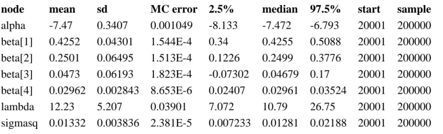
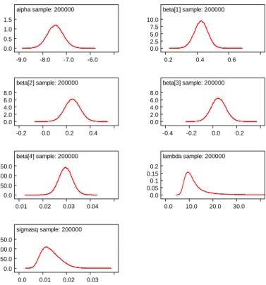
inef-ficiencies. The chain was run with a burn-in of 20 000 iterations with 200 000 retained draws and a thinning to every 5th draw. WinBUGS has a number of tools for reporting the posterior distribution. A simple summary (Table 1) can be generated showing posterior mean, median and standard deviation
with a95%posterior credible interval. Parameter names are related in an obvious way to the model in
Section 2. A fuller picture of the posterior distribution can be provided using thedensityoption in the
Sample Monitor Toolwhich draws a kernel density estimate of the posterior distribution of any chosen parameter, as in Figure 1.
node mean sd MC error 2.5% median 97.5% start sample
alpha -7.47 0.3407 0.001049 -8.133 -7.472 -6.793 20001 200000 beta[1] 0.4252 0.04301 1.544E-4 0.34 0.4255 0.5088 20001 200000 beta[2] 0.2501 0.06495 1.513E-4 0.1226 0.2499 0.3776 20001 200000 beta[3] 0.0473 0.06193 1.823E-4 -0.07302 0.04679 0.17 20001 200000 beta[4] 0.02962 0.002843 8.653E-6 0.02407 0.02961 0.03524 20001 200000 lambda 12.23 5.207 0.03901 7.072 10.79 26.75 20001 200000 sigmasq 0.01332 0.003836 2.381E-5 0.007233 0.01281 0.02188 20001 200000
Table 1:WinBUGS output for the electricity data: posterior statistics
node 2.5% median 97.5% eff[1] 1 4 90 eff[2] 34 99 123 eff[3] 13 74 121 eff[4] 9 58 120 eff[5] 25 91 122 eff[6] 23 89 122 eff[7] 21 84 122
Table 2:WinBUGS output for the electricity data: rank statistics for the first seven firms in the sample Often, the quantities of primary interest in stochastic frontier analysis are the efficiencies. Firm-specific efficiencies are immediately generated by the sampler for each firm and their full posterior distributions are readily available, and can be plotted in the same way as in Figure 1. There are
vari-ous other options for displaying the posterior distribution. For example theCompare...menu item
brings up theComparison Toolthat draws a boxplot (Figure 2) or caterpillar plot of the sampled
efficiencies for some chosen firms. A practically interesting function of the firm-specific efficiency mea-surements is given by their ranks. WinBUGS can automatically compute a sample from their posterior
alpha sample: 200000 -9.0 -8.0 -7.0 -6.0 0.0 0.5 1.0 1.5 beta[1] sample: 200000 0.2 0.4 0.6 0.0 2.5 5.0 7.5 10.0 beta[2] sample: 200000 -0.2 0.0 0.2 0.4 0.0 2.0 4.0 6.0 8.0 beta[3] sample: 200000 -0.4 -0.2 0.0 0.2 0.0 2.0 4.0 6.0 8.0 beta[4] sample: 200000 0.01 0.02 0.03 0.04 0.0 50.0 100.0 150.0 lambda sample: 200000 0.0 10.0 20.0 30.0 0.0 0.05 0.1 0.15 0.2 sigmasq sample: 200000 0.0 0.01 0.02 0.03 0.0 50.0 100.0 150.0
Figure 1: WinBUGS output for the electricity data: posterior densities for parameters
[1] [2] [3] [4] [5] [6] [7] [8] [9]
[10]
box plot: eff[1:10]
0.4 0.6 0.8 1.0
Figure 2: WinBUGS output for the electricity data: boxplot of posterior efficiency distributions for the first ten firms in the sample
distribution using theRank...option from theInferencemenu. Table 2 shows a summary of the
posterior distribution for the first seven electricity producers in the sample (high rank corresponds to high efficiencies). The posterior distribution clearly demonstrates a large spread of the rankings.
A simple check of the mixing of the posterior distribution arises from some graphical summary of the values taken by the chain. For example, a trace plot of all drawn values is available through the
historybutton or through thetracebutton for the previous batch of, say, 1000 drawings.
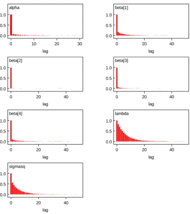
The autocorrelation function for the chain of each parameter (as shown in Figure 3) can also indicate dimensions of the posterior distribution that are mixing slowly. Slow mixing is often associated with high
alpha lag 0 10 20 30 0.0 0.5 1.0 beta[1] lag 0 20 40 0.0 0.5 1.0 beta[2] lag 0 20 40 0.0 0.5 1.0 beta[3] lag 0 20 40 0.0 0.5 1.0 beta[4] lag 0 20 40 0.0 0.5 1.0 lambda lag 0 20 40 0.0 0.5 1.0 sigmasq lag 0 20 40 0.0 0.5 1.0
Figure 3: WinBUGS output for the electricity data: autocorrelation functions of the chain posterior correlations between parameters. The plots indicate that all parameters are mixing well with
autocorrelation vanishing before 20 lags in each case. Thecorrelation tool(thecorrelation
option in theinference menu) can produce scatterplots of every parameter against every other
pa-rameter to indicate correlation or a correlation coefficient can be estimated from the current output. Graphical representations of the posterior distribution can indicate problems with the performance of the MCMC algorithm. More sophisticated methods for convergence detection are implemented in the Convergence Diagnostic and Output Analysis (CODA) software which is available for the statistical packages S-plus and R. WinBUGS produces output that is formatted for direct use with these programs and allows the behaviour of the chain to be investigated using some popular statistical tests.
Dbar = post.mean of -2logL; Dhat = -2LogL at post.mean of stochastic nodes
Dbar Dhat pD DIC
y -187.486 -233.447 45.961 -141.525 total -187.486 -233.447 45.961 -141.525
Table 3: WinBUGS output for the electricity data: DIC with normal errors
WinBUGS automatically implements the DIC (Spiegelhalter et al., 2002) model comparison crite-rion. This is a portable information criterion quantity that trades off goodness-of-fit against a model complexity penalty. In hierarchical models, deciding the model complexity may be difficult and the
of the deviance (-2 ×log likelihood) and Dˆ is a plug-in estimate of the latter based on the posterior
mean of the parameters. The DIC is computed as DIC=D¯ +pD = ˆD+ 2pD.5 Lower values of the
criterion indicate better fitting models. Table 3 records the values computed, in the same format as given by WinBUGS. For our purposes here, we will focus only on the DIC value. The method was designed to be easy to implement using a sample from the posterior distribution and the interested reader is directed to Spiegelhalter et al. (2002) for a lively discussion of its merits.
3.2
Alternative distributional assumptions
Once this model has been fitted successfully, we may want to consider further modelling options. As already indicated in Section 2, there are alternative choices of the inefficiency distribution. Another popular choice is the half-normal, which can be implemented in WinBUGS by
u[i] ˜ djl.dnorm.trunc(0,lambda,0,1000).
The prior distribution
lambda ˜ dgamma(1,1/37.5)
leads to a prior median efficiency of approximately 0.875 with a reasonable spread (see van den Broeck
et al., 1994). Yet another possible inefficiency distribution is the gamma distribution, implemented by
u[i] ˜ dgamma(phi,lambda).
A suitable prior distribution, which extends the informative prior for an exponential inefficiency distri-bution, is discussed in Griffin and Steel (2004) in a more general setting. They define
d1 <- 3 d2 <- d1 + 1
lambda0 <- -log(rstar) phi <- 1 / invphi
invphi ˜ dgamma(d1, d2)
lambda ˜ dgamma(phi, lambda0)
The prior onphihas mode at one (corresponding to the exponential), so this centres the gamma
distri-bution over the exponential distridistri-bution and the parameterd1controls the variability ofphi(a value of
3 is their suggested setting).
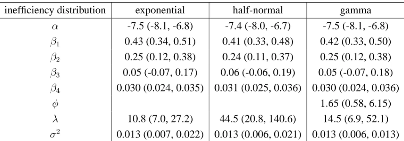
Table 4 contrasts some results on the parameters for exponential, half-normal and gamma
assump-tions. Differences on common parameters are fairly small6, and the credible interval for φ, the shape
parameter of the gamma, includes1, which corresponds to the exponential model.
In addition, a heavier tailed error distribution could be considered for the measurement error. Simply specifying
5Thus,p
Dis computed asD¯ −Dˆ.
inefficiency distribution exponential half-normal gamma α -7.5 (-8.1, -6.8) -7.4 (-8.0, -6.7) -7.5 (-8.1, -6.8) β1 0.43 (0.34, 0.51) 0.41 (0.33, 0.48) 0.42 (0.33, 0.50) β2 0.25 (0.12, 0.38) 0.24 (0.11, 0.37) 0.25 (0.12, 0.38) β3 0.05 (-0.07, 0.17) 0.06 (-0.06, 0.19) 0.05 (-0.07, 0.18) β4 0.030 (0.024, 0.035) 0.031 (0.025, 0.036) 0.030 (0.024, 0.036) φ 1.65 (0.58, 6.15) λ 10.8 (7.0, 27.2) 44.5 (20.8, 140.6) 14.5 (6.9, 52.1) σ2 0.013 (0.007, 0.022) 0.013 (0.006, 0.021) 0.013 (0.006, 0.013)
Table 4: Parameter results (posterior medians and 95% credible intervals) for various efficiency distributions with normal errors for the electricity data
y[k] ˜ dt(mu[k], prec, degfree)
changes the form of the error distribution in (1) to at-distribution withdegfreedegrees of freedom.
The prior distribution for the degrees of freedom was chosen to be exponential with mean and standard
deviation equal to3:
degfree ˜ dexp(0.333),
which puts a considerable amount of prior mass on distributions with much heavier tails than the normal distribution.
inefficiency distribution exponential half-normal gamma α -7.8 (-8.4, -7.1) -7.7 (-8.4, -7.0) -7.8 (-8.4,-7.1) β1 0.45 (0.36, 0.52) 0.44 (0.35, 0.52) 0.44 (0.35, 0.52) β2 0.29 (0.16, 0.42) 0.28 (0.16, 0.41) 0.29 (0.16, 0.42) β3 0.04 (-0.07, 0.16) 0.05 (-0.06, 0.17) 0.04 (-0.07, 0.16) β4 0.028 (0.023, 0.034) 0.029 (0.023, 0.034) 0.023 (0.028, 0.034) ν 4.4 (2.0, 11.8) 3.5 (1.6, 10.3) 4.0 (1.7, 11.1) φ 1.9 (0.7, 6.9) λ 11.3 (7.1, 29.4) 43.8 (20.8, 141.1) 16.0 (7.5, 56.1) σ2 0.008 (0.003, 0.016) 0.006 (0.001, 0.014) 0.002 (0.0004, 0.0073)
Table 5: Parameter results (posterior medians and 95% credible intervals) for the two alternative efficiency
distribu-tions withterrors for the electricity data
Table 5 records some results and illustrates that the prior assumption about the degrees of freedom,
indicated byν, is quite important since the data provide little information about its value. We can use
the DIC criterion to compare the different models. Table 6 compares the DIC scores for the possible combinations of error distribution and inefficiency distribution. Smaller values of the DIC suggest better
error distribution inefficiency distribution D¯ Dˆ pD DIC normal exponential -187.5 -233.4 46.0 -141.5 half-normal -189.3 -239.5 50.2 -139.1 gamma -187.7 -234.0 46.4 -141.3 t exponential -190.7 -238.8 48.1 -142.6 half-normal -209.7 -263.3 53.6 -156.1 gamma -198.7 -247.7 49.0 -149.7 Table 6:Comparison of models with different distributional assumptions using the DIC criterion
eff[124] sample: 200000 0.2 0.4 0.6 0.8 1.0 0.0 2.0 4.0 6.0
Figure 4: WinBUGS output for the electricity data: kernel density estimate of the posterior predictive efficiency
distribution for the Student-tmodel with half-normal efficiencies
models and so the Student-terrors tend to fit the data better than the normal measurement errors. Overall,
the results favour the half-normal distribution witht-distributed errors. The posterior distribution of the
mean of the predictive (i.e. out-of-sample) efficiency is a useful measure for comparing our inference
about the parameters of the inefficiency distributionsλandφ(presented in Table 5). Ift-distributed errors
are assumed, the posterior mean of predictive efficiency has a 95% credibility interval of (0.88,0.97) for the exponential distribution, (0.80,0.96) for the gamma and (0.85,0.94) for the half-normal distribution. In other words, for this data, the half-normal and gamma distributions are associated with slightly lower estimates of efficiency than the exponential distribution.
Finally, we estimate the posterior predictive distribution of efficiency for our preferred model with
t-distributed measurement errors and a half-normal efficiency distribution. This corresponds to the
effi-ciency of an unobserved firm in this sector. An extra ineffieffi-ciency node (u[N+1]) and efficiency node
(eff[N+1]) are added to the model by defining
for (i in 1:(N+1)) {
u[i] ˜ djl.dnorm.trunc(0,lambda,0,1000) eff[i] <- exp(- u[i])
}
A kernel density estimate of the distribution is shown in Figure 4. Posterior predictive median efficiency is 0.91 and the 95% credible interval is (0.69,0.996).
3.3
Imposing regularity conditions
The fitted frontier should obey certain economic constraints (see e.g. Kumbhakar and Lovell 2000). For example, a cost frontier should imply positive elasticities of cost with respect to output and prices. In other word, we need to check
d lnC
dlnXi >0.
If a Cobb-Douglas frontier is fitted the condition reduces to positive coefficients in the frontier. This
change can be easily implemented in the prior distribution ofβiby replacing the normal prior
beta[i] ˜ dnorm(0.0, 1.0E-06)
with its truncated counterpart
beta[i] ˜ djl.dnorm.trunc(0.0, 1.0E-0.6,0,1000).
However, a more complicated frontier such as a translog will lead to more complicated expressions for
dlnC/dlnXi. In this example, a quadratic output term is included in the frontier and the elasticity of
cost with respect to output has the form
d lnC
d lnQ =β1+ 2β4lnQ.
Ideally, we would want this relationship to be true for all values oflnQ. However, since this is only
a local approximation to the frontier, it is usual to check the condition for a plausible set of values of
lnQ. A pragmatic approach restricts attention to the value of the elasticity for the observed output. This
approach will be used in this case. Imposing these properties in alternative sets of values as in Terrell
(1996) can easily be implemented. The restrictions are imposed onp(y|X, β)leading to a non-standard
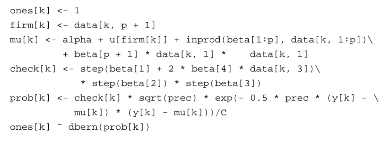
likelihood function, which is implemented using the “ones-trick” described in the WinBUGS manual.
This introduces a new variablecheck, which will be zero for all cases where regularity conditions are
violated and one elsewhere. The data is now a set of ones assumed to be the result of Bernoulli sampling with probabilities proportional to the likelihood values of those observations for which regularity holds and zero for which it is violated. As soon as a violation occurs for one of the observations, the likelihood
value associated with that draw will, thus, be zero. C is a constant such that all values in prob are
smaller than one. In particular, we replace
for ( k in 1:K ) {
firm[k] <- data[k, p + 1]
mu[k] <- alpha + u[firm[k]] + inprod(beta[],data[k,1:p]) y[k] ˜ dnorm(mu[k], prec)
}
by
C<- 10000
ones[k] <- 1
firm[k] <- data[k, p + 1]
mu[k] <- alpha + u[firm[k]] + inprod(beta[1:p], data[k, 1:p])\ + beta[p + 1] * data[k, 1] * data[k, 1]
check[k] <- step(beta[1] + 2 * beta[4] * data[k, 3])\ * step(beta[2]) * step(beta[3])
prob[k] <- check[k] * sqrt(prec) * exp(- 0.5 * prec * (y[k] - \ mu[k]) * (y[k] - mu[k]))/C
ones[k] ˜ dbern(prob[k]) }
where the more general form ofmuis used throughout this section and is simply a consequence of the
specific cost frontier in (3) and\indicates that the following line is the continuation of the current line
and both should be entered as a single line.
inefficiency distribution exponential half-normal α -7.7 (-8.2, -7.0) -7.7 (-8.3, -7.0) β1 0.44 (0.35, 0.52) 0.44 (0.35, 0.52) β2 0.27 (0.16, 0.37) 0.27 (0.15, 0.39) β3 0.06 (0.00, 0.16) 0.06 (0.00, 0.17) β4 0.028 (0.023, 0.034) 0.028 (0.023, 0.034) ν 4.4 (2.1, 11.8) 3.6 (1.6, 10.4) λ 11.3 (7.1, 29.4) 43.6 (20.6, 140.9) σ2 0.008 (0.003, 0.016) 0.006 (0.001, 0.014)
Table 7: Parameter results (posterior medians and 95% credible intervals) for two inefficiency distributions witht
errors for the electricity data with economic restrictions
It should be noted that the non-standard likelihood function can lead to a severe deterioration in the performance of the Gibbs sampler that WinBUGS implements, which can lead to slow convergence and mixing. In this example, we used a thinning of 100 which lead to good autocorrelation properties in the chain. Table 7 presents results for two possible choice of inefficiency distribution. Comparison with Table 5 shows that the economic constraints are rarely violated for these data and the implementation
of economic constraints in this example has little effect on the analysis. Only the inference onβ3 is
moderately affected.
4
A Panel of US Hospital data
Our second example reanalyses data on costs of US hospitals initially conducted in Koop, Osiewalski and Steel (1997), and we refer to the latter paper for further details and background of hospital cost
estimation, the data and the particular frontier used. The data correspond toN = 382 nonteaching
U.S. hospitals over the years 1987-1991 (T = 5), selected so as to constitute a relatively homogeneous
sample. The frontier describing cost involves five different outputsY1, . . . , Y5: number of cases, number
of inpatient days, number of beds, number of outpatient visits and a case mix index. We also include
a measure of capital stock, C, an aggregate wage index, P, and a time trendtto capture any missing
dynamics. We choose a flexible translog specification and impose linear homogeneity in prices, which allows us to normalize with respect to the price of materials. Thus, in the notation of (1) and dropping
observational subscripts for ease of notation,y= ln(cost) andx0βbecomes:
x0β= 5 X i=1 βilnYi+β6lnP +β7(lnP)2+ 5 X i=1 β7+ilnYilnP +β13lnC + 5 X i=1 β13+ilnYilnC+β19lnPlnC+β20(lnC)2+β21t+β22t2 + 5 X i=1 5 X j=i β22+5(i−1)+jlnYilnYj.
Throughout this section, we will use the normal sampling in (1) combined with an exponential ineffi-ciency distribution.
4.1
Including covariates in the inefficiency distribution
Koop, Osiewalski and Steel (1997) consider a method for extending the stochastic frontier to allow exponentially distributed inefficiencies to depend upon covariates. Their model assumes that each firm
has a vector of binary covariates,wifor thei-th firm. That firm’s inefficiency is modelled as
ui∼Exp(exp{wiγ}). (4)
whereγ is a vector of regression coefficients. In the current example, there are 3 possible ownership
categories for each firm and so w contains dummy variables to represent category membership.
Ac-tually, since WinBUGS does not rely on known forms for the conditionals, the covariateswi can also
include non-binary variables. It seems reasonable to assume a priori that our belief about the efficiency distribution for each category should be the same, i.e.
exp{γj} ∼Exp(−logr?).
This model can be coded by defininglambda[i], the inverse of mean inefficiency for thei-th firm and
data2a matrix containing each firm’s characteristicsw.
for (i in 1:N) {
lambda[i] <- exp(inprod(gamma[], data2[i, 1:p2]))
u[i] ˜ dexp(lambda[i]) eff[i] <- exp(- u[i]) }
It is easier to define a prior distribution forexp{γj}and WinBUGS allows us to define the relationship
gamma[j] <- log(expgamma[j])using a logical node. The WinBUGS code for this prior is:
lambda0 <- -log(rstar) for ( j in 1:p2 ) {
gamma[j] <- log(expgamma[j]) expgamma[j] ˜ dexp(lambda0) }
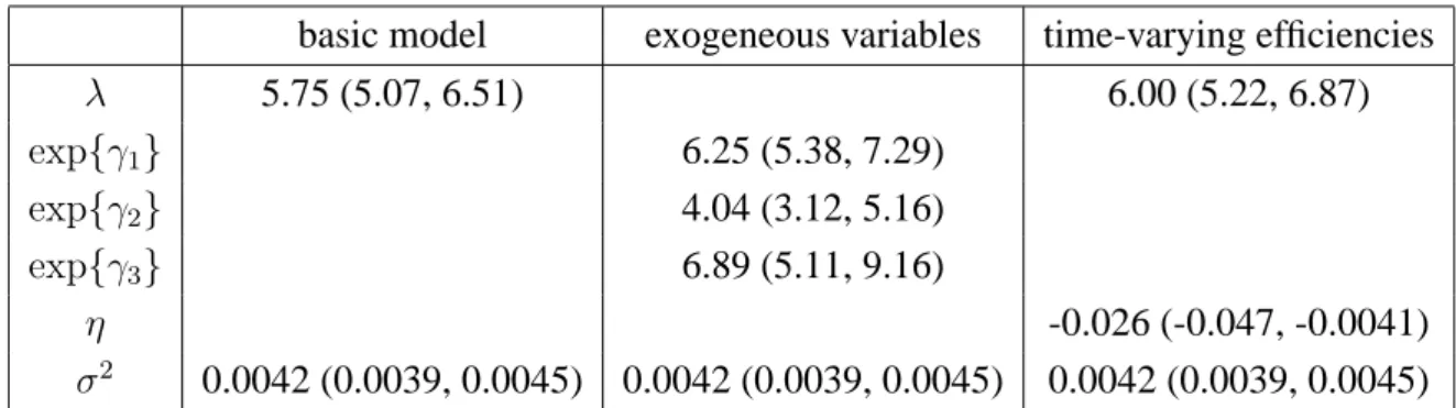
Using ownership dummies (indicating non-profit, for-profit or government-run hospitals) as covari-ates for the inefficiency distribution, Table 9 compares the DIC values for the basic model with that of the model including these covariates. There seems to be little support for this model extension. Never-theless, Table 8 does indicate some evidence for lower efficiencies in the for-profit sector (corresponding
toγ2). The latter is in line with the results in Koop, Osiewalski and Steel (1997).
basic model exogeneous variables time-varying efficiencies
λ 5.75 (5.07, 6.51) 6.00 (5.22, 6.87) exp{γ1} 6.25 (5.38, 7.29) exp{γ2} 4.04 (3.12, 5.16) exp{γ3} 6.89 (5.11, 9.16) η -0.026 (-0.047, -0.0041) σ2 0.0042 (0.0039, 0.0045) 0.0042 (0.0039, 0.0045) 0.0042 (0.0039, 0.0045)
Table 8: Selected parameter results (posterior medians and 95% credible intervals) for the hospital data
¯
D Dˆ pD DIC
basic model -5033 -5413 379.7 -4654 exogeneous variables -5025 -5403 378.0 -4647 time-varying -5041 -5423 381.5 -4660
Table 9: DIC results for the hospital data with various model specifications
4.2
Time-varying efficiency
The assumption made in equation (2) that firm-specific technical efficiency is constant over time may
not always be tenable. An alternative model that allows time-varying efficiencies usesuit to represent
the inefficiency of firm i at time t. A simplifying assumption proposed in Lee and Schmidt (1993)
definesuit=β(t)ui.This specification is parsimonious but makes a strong assumption about the form of
time-dependence. Several forms have been considered forβ(t), in particular Battese and Coelli (1992)
propose
where positive η indicates increasing efficiency over time. We choose the prior distribution of η to be a zero-mean normal distribution with variance 0.25 which represents our prior indifference between
increasing and decreasing efficiency and, for T = 5, supports reasonable predictive distributions of
efficiency at each time point. This new model can be implemented in WinBUGS by changing the mean of the log costs to
t <- data[k, p+2]
mu[k] <- alpha + exp(eta*(t-T)) * u[firm[k]] + inprod(beta[],data[k,1:p])
and the prior is represented by the statement
eta ˜ dnorm(0.0,4).
Table 9 indicates some support for this time-varying model over the basic model. From the posterior
results onηin Table 8, we conclude that efficiencies tend to decrease somewhat over time.
4.3
Model comparison of the form of the frontier
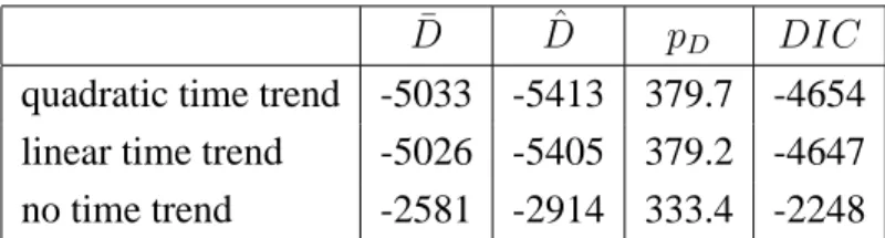
The stochastic frontier represents an approximation to the best-practice output for a set of inputs or lowest cost for producing a set of outputs. The common forms of the function have usually been log-linear but there may be uncertainty in the frontier specification. For example, a Cobb-Douglas functional form is fairly restricted. A translog is much more flexible, using a second order approximation to the unknown function, but at the expense of introducing many parameters which can lead to a poor fit. An improvement in fit may arise through careful selection of the higher order terms and interactions or of various other covariates. In the example above, we might wish to allow for the possibility of no time trend, a linear time trend or a quadratic time trend. In the Bayesian approach these questions of model choice can be answered through model comparison tools such as the DIC. We restrict attention to deciding on the type of time trend to include in the model. Table 10 shows the results of running three separate chains incorporating no time trend, a linear trend and a quadratic time trend in the basic model with a common efficiency distribution for all hospital types and constant efficiencies over time. The models with a time trend far outperform the model without time trend. The results indicate a preference for the model with a quadratic time effect, as used in the previous subsections.
¯
D Dˆ pD DIC
quadratic time trend -5033 -5413 379.7 -4654 linear time trend -5026 -5405 379.2 -4647 no time trend -2581 -2914 333.4 -2248 Table 10: DIC results for the hospital data with the basic model
5
Conclusions
This paper demonstrates that WinBUGS provides a useful framework for the Bayesian analysis of stochastic frontier models. We provide code to implement a standard model for cross-sectional, bal-anced and unbalbal-anced panel data with a time-invariant exponential inefficiency distribution. Many other, more complicated, models can be analysed using simple extensions of this code, for example to include covariates in the efficiency distribution and time-varying efficiencies. We also illustrate ways to impose economic regularity conditions and deal with model uncertainty. We emphasize that we have merely
shown a few possible model specifications and extensions7and it should also be fairly straightforward
to implement many other Bayesian models such as random coefficient frontiers (see Tsionas, 2002 and Huang, 2004) or models developed in the literature for dealing with multiple-output analysis or the mod-elling of undesirable outputs (see Fern´andez, Koop and Steel, 2002). We also stress that priors can be specified in line with genuine prior beliefs, as WinBUGS does not require priors to be conjugate in any sense. Modelling, both of the sampling model and the prior assumptions, can be conducted creatively and in accordance with the particular problem at hand, without worrying about having to develop and modify complicated computer code.
WinBUGS immediately leads to full posterior distributions of the model parameters and interest-ing functions of these parameters, such as firm-specific efficiencies and the rankinterest-ings of firm-specific efficiencies. Many graphical and other summaries of the posterior distributions and the behaviour of the MCMC sampler are built-in. The availability of CODA-compatible output allows a range of convergence diagnostics to be produced very easily.
We would certainly recommend the applied user of stochastic frontier models to experiment with WinBUGS and we hope that the availability of WinBUGS code will allow these users to add Bayesian methods to their modelling and inference toolbox.
References
Aigner, D., C.A.K. Lovell and P. Schmidt. (1977). “Formulation and estimation of stochastic frontier production function models.” Journal of Econometrics 6, 21-37.
Arickx, F., J. Broeckhove, M. Dejonghe and J. van den Broeck. (1997). “BSFM: A Computer Program for Bayesian Stochastic Frontier Models.” Computational Statistics 12, 403-421.
Battese, G.E. and T.J. Coelli. (1992). “Frontier Production Functions, Technical Efficiency and Panel Data: With Application to Paddy Farmers in India.” Journal of Productivity Analysis 3, 153-169. Christensen, L. R. and W. H. Greene (1976). “Economies of Scale in U.S. Electric Power Generation.”
Journal of Political Economy 84, 655-676.
Ennsfellner, K.C., D. Lewis D and R.I. Anderson. (2004). “ Production efficiency in the Austrian insurance industry: A Bayesian examination.” Journal of Risk and Insurance 71, 135-159.
Fern´andez, C., G. Koop and M. F. J. Steel. (2002). “Multiple Output Production with Undesirable Outputs: An Application to Nitrogen Surplus in Agriculture,” Journal of the American Statistical
Association, 97, 432-442.
Greene, W.H. (1990). “A Gamma-Distributed Stochastic Frontier Model.” Journal of Econometrics 46, 141-163.
Griffin, J. E. and Steel, M. F. J. (2004). “Flexible Mixture Modelling of Stochastic Frontiers.” Univer-sity of Warwick, Technical Report.
Huang, H.C. (2004). “Estimation of technical inefficiencies with heterogeneous technologies.” Journal
of Productivity Analysis 21, 277-296.
Kim, Y. and P. Schmidt (2000). “A review and empirical comparison of Bayesian and classical ap-proaches to inference on efficiency levels in stochastic frontier models with panel data.” Journal
of Productivity Analysis, 14, 91-118.
Koop, G., J. Osiewalski and M.F.J. Steel (1997). “Bayesian Efficiency Analysis Through Individual Effects: Hospital Cost Frontier.” Journal of Econometrics, 76, 77-105.
Koop, G, M.F.J. Steel and J. Osiewalski. (1995). “Posterior analysis of stochastic frontier models using Gibbs sampling.” Computational Statistics, 10, 353-373.
Kumbhakar, S.C. and Lovell, C.A.K. (2000). Stochastic Frontier Analysis. Cambridge University Press: New York.
Kumbhakar, S.C. and E.G. Tsionas. (2005). “Measuring technical and allocative inefficiency in the translog cost system: a Bayesian approach.” Journal of Econometrics, 126, 355-384.
Kurkalova L.A. and A. Carriquiry. (2002). “An analysis of grain production decline during the early transition in Ukraine: A Bayesian inference.” American Journal of Agricultural Economics 84, 1256-1263.
Lee, Y. H. and P. Schmidt (1993). “A production frontier model with flexible temporal variation in technical efficiency.” in H. O. Fried, C. A. K. Lovell, and S. S. Schmidt, eds. The Measurement of
Productive Efficiency: Techniques and Applications. New York: Oxford University Press.
Meeusen, W. and J. van den Broeck. (1977). “Efficiency estimation from Cobb-Douglas production functions with composed errors.” International Economic Review, 8, 435-444.
Spiegelhalter D. J., N. G. Best, B. P. Carlin and A. van der Linde (2002). “Bayesian measures of model complexity and fit (with discussion).” Journal of the Royal Statistical Society B, 64, 583-640. Stevenson, R.E. (1980). “Likelihood functions for generalized stochastic frontier estimation.” Journal
of Econometrics 13, 57-66.
Terrell, D. (1996). “Incorporating monotonicity and concavity conditions in flexible functional forms.”
Journal of Applied Econometrics 11, 179-194.
Tsionas, E. G. (2000). “Full likelihood inference in Normal-gamma stochastic frontier models.”
Tsionas, E. G. (2002). “Stochastic Frontier Models with Random Coefficients.” Journal of Applied
Econometrics, 17, 127-147.
van den Broeck, J., G. Koop, J. Osiewalski and M.F.J. Steel. (1994). “Stochastic Frontier Models: A Bayesian Perspective.” Journal of Econometrics, 61, 273-303.
![Table 6: Comparison of models with different distributional assumptions using the DIC criterion eff[124] sample: 200000 0.2 0.4 0.6 0.8 1.0 0.0 2.0 4.0 6.0](https://thumb-us.123doks.com/thumbv2/123dok_us/9897071.2483254/11.892.167.736.136.319/table-comparison-models-different-distributional-assumptions-criterion-sample.webp)