GENERATION OF GREY PATTERNS USING AN IMPROVED
GENETIC-EVOLUTIONARY ALGORITHM: SOME NEW RESULTS
hAlfonsas Miseviius
Kaunas University of Technology, Department of Multimedia Engineering, Student St. 50400a/416a, LT51368 Kaunas, Lithuania
e-mail: [email protected]
Abstract. Genetic and evolutionary algorithms have achieved impressive success in solving various optimization problems. In this work, an improved genetic-evolutionary algorithm (IGEA) for the grey pattern problem (GPP) is discussed. The main improvements are due to the specific recombination operator and the modified tabu search (intra-evolutionary) procedure as a post-recombination algorithm, which is based on the intensification and diversification methodology. The effectiveness of IGEA is corroborated by the fact that all the GPP instances tested are solved to pseudo-optimality at very small computational effort. The graphical illustrations of the grey patterns are presented.
Keywords: combinatorial optimization; heuristics; genetic-evolutionary algorithms; grey pattern problem.
h This work was supported by Lithuanian State Science and Studies Foundation (grant number T-09293). Introduction
The grey pattern problem (GPP) [29] deals with a rectangle (grid) of dimensions n1un2 containing n = n1un2 points (m black points and nm white points). By putting together many of these rectangles, one gets a grey pattern (frame) of density m/n (see Figure 1). The goal is to get the most excellent grey pattern, that is, the points have to be spread on the rectangles as smoothly as possible.
Figure 1. Examples of grey frames: m/n = 58/256 (a), m/n = 198/256 (b)
Formally, the GPP can be stated as follows. Let two matrices A = (aij)nun and B = (bkl)nun and the set 3 of all possible permutations of the integers from 1 to n
be given. The objective is to find a permutation S= (S(1), S(2), ..., S(n)) 3 that minimizes
¦¦
n in
j
j i ijb a z
1 1
) ( ) ( )
(S S S , (1)
where the matrix (aij)nun is defined as aij = 1 for i, j =1, 2, ..., m and aij = 0 otherwise; the matrix (bkl)nun is defined by the distances between every two of n
points. More precisely, bkl bn2(r1)s n2(t1)u frstu, where
2 2 2
1 }
1 , 0 , 1 {
, ( ) ( )
1 max
w n u s v n t r f
w v rstu
,
r, t = 1, ..., n1, s, u = 1, ..., n2. (2)
frstu may be thought of as an electrical repulsion force between two electrons (to be put on the grid points) i
and j (i, j = 1, ..., n) located in the positions k = S(i) and l = S(j) with the coordinates (r, s) and (t, u). The
ith (idm) element of the permutation S, S(i)= n2(r 1) + s, gives the location in the rectangle where a black point has to be placed in. The coordinates of the black point are derived according to the formulas: r = ¬(S(i) 1)/n2¼ + 1, s = ((S(i) 1) mod n2) + 1, where S(i) denotes the location of the black point, i = 1, 2, ..., m [29].
The grey pattern problem is a special case of the quadratic assignment problem (QAP) [4, 11], which is known to be NP-hard. Recently, genetic and evolutio-nary algorithms (GAs, EAs) are among the most ad-vanced heuristic approaches for these problems [5, 15, 17, 18, 24, 29]. GAs and EAs belong to a class of po-pulation-based heuristics. The following are the main phases of the genetic-evolutionary algorithms. Usual-ly, a pair of individuals (solutions) of a population is
(a) (b)
selected to be parents (predecessors). A new solution (i.e. offspring) is created by recombining (merging) the parents. In addition, some individuals may under-go mutations. Afterward, a replacement (reproduction) scheme is applied to the previous generation and the offspring to determine which individuals survive to form the next generation. Over many generations, less fit individuals tend to die-off, while better individuals tend to predominate. The process continues until a ter-mination criterion is met. For a more thorough discus-sion on the principles of GAs and EAs, the reader is addressed to [2, 8, 9, 12].
This work is organized as follows. In Section 1, the improved genetic-evolutionary algorithm (IGEA) framework is discussed. The details of IGEA for the grey pattern problem are described in Section 2. In Section 3, we present the results of generation of grey patterns using two versions of the proposed algorithm. Section 4 completes the work with conclusions.
1. The improved genetic-evolutionary algorithm framework
The original concepts of GAs and EAs were introduced by Holland [10], Rechenberg [25] and Schwefel [26] in the nineteen seventies. Since that time, the structure of GAs and EAs has experienced various transformations. The state-of-the-art genetic-evolutionary algorithms are in fact hybrid algorithms, which incorporate additional heuristic procedures [21, 22, 23]. However, applying hybridized algorithms does not necessarily imply that good solutions are achieved at reasonable time [17]. Indeed, hybrids often make use of refined heuristics (like simulated annealing, tabu search) which are quite time-expen-sive. This may become in real earnest a serious draw-back, especially as we are willing to construct algo-rithms that are competitive with other intelligent opti-mization techniques. Under these circumstances, it is important to add additional enhancements to the gene-tic-evolutionary algorithms (see also [17]).
The enhanced hybrid genetic-evolutionary algo-rithms should incorporate fast local improvement procedures. Only short time behaviour matters as long as we are speaking of the fast procedures in the context of hybrid GA/EAs.
The compactness of the population is of great importance. In the presence of powerful local impro-vement procedures, the large populations are not necessary: the small population size is fully compen-sated by the improvement heuristic.
A high degree of the diversity within the popu-lation must be maintained. This is especially true for tiny populations. Indeed, the smaller the size of the population, the larger the probability of the lost of diversity. Therefore, proper mechanisms for avoiding premature convergence must be applied.
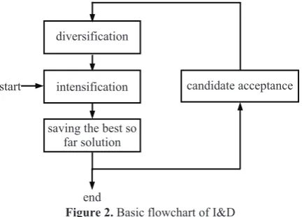
Figure 2. Basic flowchart of I&D
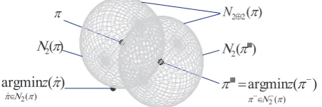
The principle that can help putting the above en-hancements into practice is known as "intensification and diversification" (I&D) [7]. The idea behind is to seek high quality solutions by iterative applying local search ("recreation") and perturbation ("ruin") proce-dures. I&D is initiated by improvement of a starting solution. Then, one perturbs the existing solution (or its part). After that, the solution is again improved by means of a local search algorithm, and so on. I&D is distinguished for three main components: intensifica-tion, diversificaintensifica-tion, and candidate acceptance crite-rion (see Figure 2). The goal of intensification is to concentrate the search in a localized area (the neigh-bourhood of the current solution). Diversification is responsible for escaping regions of "attraction" in the search space. It may be achieved by certain perturba-tions of soluperturba-tions (instead of saying "perturbation", other terms may be utilized: "mutation", "ruin", etc.). Finally, an acceptance criterion is used to decide which solution is actually chosen for the subsequent perturbation (see Section 2.4.3). I&D may be incor-porated into the genetic-evolutionary algorithm in two ways.
Firstly, I&D is applied to single solutions, in particular, to the offspring obtained by parent recom-bination. We call this post-recombination procedure the intra-evolutionary process (or simply intra-evolution). Intra-evolution could be seen as a very special case of the conventional evolutionary algo-rithm, that is, the population size is equal to 1, the reproduction scheme is "1, 1" (or "1 + 1"), and the single solution mutation procedure is used instead of the recombination operator. The mutation procedure plays, namely, the role of diversification. Regarding intensification, we found the tabu search (TS) tech-nique [7] ideal for the GPP. The details of the TS pro-cedure are described in Section 2.4.1.
Secondly, I&D may also be applied for the po-pulations. In this case, it is enough to think of the population as some kind of meta-solution; that is, instead of improvement/perturbation of the single solution, the meta-solution, i.e. population is to be improved/perturbed. Basically, this means that the whole population (or, at least, its part) undergoes some deep mutation. In particular, the test is performed at
candidate acceptance diversification
intensification start
end saving the best so
every generation, whether the diversity within the current population is below a given threshold. If it is, then a new population is created by applying muta-tions and following improvement; otherwise, the search is continued with the current population in an ordinary way. We call the above process the inter-evolution.
2. The improved genetic-evolutionary algorithm for the grey pattern problem
2.1. Creation of the initial population
The initial population (say, P) is created in two phases: firstly, PS = | P | individuals, i.e. the GPP solutions are generated in a pure random way; se-condly, all the solutions of the produced population are improved by the intra-evolutionary algorithm (see Section 2.4). As a result, the population is created that consists solely of locally optimal solutions. Even-tually, the population members are sorted according to the increasing values of the objective function.
2.2. Selection mechanism
Two individuals are selected to be predecessors of a new recombined individual. For the selection, we apply a rank based rule [31]. In particular, the position of the first parent, u1, within the sorted population is determined by the formula: u1 = ¬vV¼, where v is a uniform random number from the interval [1, PS1V], where PS is the population size, and V is a real number in the interval [1, 2] (it is referred to as a selection factor). The same formula is utilized for defining of the position for the second parent, u2 (u2zu1). It is obvious that the larger value of V, the more probability that the better individual will be selected for recombination.
2.3. Recombination of solutions
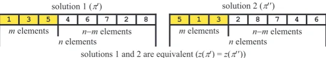
Recombination of solutions remains one of the key factors by constructing competitive genetic/evolu-tionary algorithms. Very likely, the role of recombina-tion operators within the hybrid algorithms is even more important. The classical recombination operators like one point [8] or uniform [28] operators are not very well fitted for the grey pattern problem. This is
due to the fact that basically only the first m elements (black points) determine the solution of the GPP (see Figure 3). The interchange of any of the first m
elements does not influence the objective function value (the same is true for the last nm elements (white points)).
Recombination is a structured process that ensures that the offspring will inherit the elements (genes) which are common to both parents. We can also think of recombination as a special sort diversification inst-rument; that is, it is desirable that recombination would add some randomness (certain elements, which are not contained in the parents, should be incorpora-ted into the offspring). The degree of "disruptiveness" is introduced to formally describe a measure of how much recombination is randomized, i.e. how many "foreign genes" there are in the offspring (see also [17]). The degree of disruptiveness, U, is defined as follows:
{ | ( ) { (1), (2),..., ( )} ( )
{ (1), (2),..., ( )}},
i i m i m i
m
U S S S S S
S S S
c c c
d q q
cc cc cc (3)
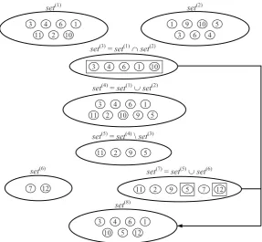
where Sc, Scc are the parents and Sq is the offspring. There are two situations: 1) U = 0; 2) U > 0. We assume that the second variant is preferable to the first one in the environment of the robust hybrid algorithm. In our algorithm, disruptiveness is flexibly controlled by adding ¬[m¼ foreign genes to the offspring, where [ is a parameter (disruptiveness factor). The recombi-nation procedure itself is quite specific. It is based on the merging process suggested in [3, 5]. The detailed pseudo-code of this recombination procedure (written in an algorithmic language) is presented in Figure 4. An illustrative example is shown in Figure 5.
It should be noted that the heuristic procedure based on tabu search is incorporated into the recom-bination process to partially improve the offspring. This procedure is performed on a restricted set of the elements of the offspring. The details of the improve-ment process are considered in the next section. Also, note that we apply the above recombination process more than once at one generation. In our implemen-tation, the number of recombinations per generation is controlled by the parameter Nrecomb.
Figure 3. The case of solutions of the grey pattern problem
1 3 5 4 6 7 2 8
m elements nm elements n elements
solution 1 (Sc)
solutions 1 and 2 are equivalent (z(Sc) = z(Scc))
5 1 3 2 8 7 4 6
m elements nm elements n elements
Figure 4. Pseudo-code of the recombination procedure for the GPP
Figure 5. Example of creating a starting offspring procedure Recombination;
// input: Sc, Scc solutions-parents, n problem size, m number of black points, [1, [2 disruptiveness factors // output: Sq recombined solution (offspring)
U1 := max{1, ¬[1m¼}; U2 := max{1, ¬[2m¼};
obtain set(1) from the first m elements of Sc; // |set(1)| = m
obtain set(2) from the first m elements of Scc; // |set(2)| = m
if not(set(1){set(1)) then begin // the sets set(1) and set(2) are different
set(3) := set(1)set(2); mintersect = |set(3)|; set(4) := set(1)set(2); // mintersect> 0, munion = |set(4)| = 2mmintersect set(5) := set(4) \ set(3); // mdifference = |set(5)| = 2m 2mintersect
if 2mmintersect + U1dn then U := U1 else U := n 2m + mintersect;
select U different elements from Sc not in set(4) to form set(6);
set(7) := set(5)set(6); mnew = |set(7)|; // mnew = min{2m 2mintersect + U, nmintersect}
add mmintersect random elements from set(7) to set(3) to create set(8); // set(8) contains exactly m elements that serve as the starting offspring
if mnew (mmintersect) > 0 then begin
obtain S from the elements of set(8); obtain S from the elements of set(7) that are not in set(8); merge S and S to get S, the number of elements of S is equal to mnewmintersect;
if mnew (mmintersect) d 5 then apply FastSteepestDescent to S, get Sˆ else apply FastRandomizedTabuSearch to S, get Sˆ
// note: FastSteepestDescent and FastRandomizedTabuSearch are performed // only on the elements in set(7) and keeping the elements in set(3) fixed
end
else obtain Sˆ from the elements of set(8)
end
else begin // the sets set(1) and set(2) are equivalent
select U2 different elements from Sc not in set(1) to create set(3);
remove U2 random elements from set(1); obtain Sˆ from the elements of set(1) and set(3)
end;
obtain S from the elements of set {1, 2, …, n} \ {Sˆ(1),Sˆ(2),...,Sˆ(m)}; merge Sˆ and S to get the offspring Sq
end.
3 4 6 1 11 2 10
set(1)
|set(1)| = 7, |set(2)| = 7, |set(3)| = 5, |set(4)| = 9, |set(5)| = 4, |set(6)| = 2, |set(7)| = 6, |set(8)| = 7
1 9 10 5
3 6 4
set(2)
set(4)=set(1)set(2)
3 4 6 1
2 10 9 5
11
set(5)=set(4)\set(3)
11 2 9 5
3 4 6 1
10 5 12
set(8) set(6)
7 12
set(7) = set(5) set(6)
11 2 9 5 7 12
set(3) = set(1) set(2)
Figure 6. Example of the pairwise interchange
2.4. Local improvement (intra-evolution)
The post-recombination improvement is probably the most important component of IGEA. In the simp-lest case, we could utilize the ordinary descent local search for this purpose. But we should make use of more elaborated approaches like tabu search if we are seeking for superior quality results. The standard TS algorithms, however, suffer from cycling and stagna-tion phenomena. Fortunately, there exist the I&D ap-proach (see Section 1). If intensification is performed, namely by means of the conventional TS, one gets the so-called iterated tabu search (ITS) method [20]. There are three main ingredients in the ITS approach: tabu search, mutation, and acceptance criterion.
2.4.1. Tabu search procedure
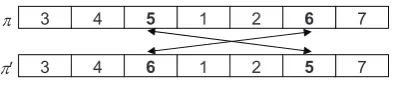
The central idea of tabu search is allowing clim-bing moves when no improving solution exists (this is in contrast to the descent local search, which terminates as soon as the locally optimal solution has been encountered). TS starts from an initial solution, and moves repeatedly from the current solution to a neighbouring one. We use the 2-exchange neigh-bourhood, 12, where the neighbours are obtained by pairwise interchanges of the elements of a solution (see Figure 6). Formally, the neighbourhood 12 of the solution S is defined by the formula:
S S S S
1 ( ) { |
2 pij ,S3 ,i 1,... ,m,j m1,...,n};
here, S Spij means that
S is obtained from S by applying the move pij (the move pij exchanges the ith and the jth element in the given permutation, i.e.
) ( ) (i S j
S S(j) S(i)).
At each step of TS, a set of the neighbours of the current solution is considered and the move that improves most the objective function value is chosen. If there are no improving moves, TS chooses one that least degrades the objective function. The reverse moves to the solutions just visited are to be forbidden in order to avoid cycling. The GPP allows imple-menting the list of tabu moves in an effective manner. In particular, the tabu list is organized as an integer matrix T= (tij)mu(nm). At the beginning, all the entries of T are set to zero. As the search progresses, the entry
tij stores the current iteration number, plus the value of the tabu tenure, h, i.e. the number of the future iteration starting at which the ith and the jth elements may again be interchanged. In this case, an elementary perturbation (move) pij is tabu if the value of tij is equal or greater than the current iteration number. Note that testing whether a move is tabu or not
requires only one comparison. We therefore call the above procedure the fast tabu search procedure.
An aspiration criterion allows permitting the tabu status to be ignored under favourable circumstances. Usually, the move from the solution S to solution S¡ is permitted (even if S¡ is tabu) if z(S¡) < z(S), where S is the best solution found so far. The resulting decision rule looks thus as follows: replace the current solution S by the new solution Si such that Si=argmin ( )
) (
2 ¡
¡
¡ 1 S S
S
z ,
where 1 S2( ) {S |S 1 S2( ) and ((S is not
¡ ¡ ¡ ¡
tabu) or ( (z S¡)z(S)))}.
TS forbids some moves from time to time. This fact means that certain portions of the search space are excluded from being visited. This can be seen as a disadvantage of the search process. One of the possible ways to get over this weakness is to minimize these restrictions, that is, it is desirable that the num-ber of forbidden moves is as minimal as possible. We propose a very simple trick: the tabu status is disre-garded with a small probability even if the aspiration criterion does not hold. We empirically found that the proper value of this probability, D, is somewhere between 0.05 and 0.1 (we used D = 0.05). As the tabu status is ignored randomly with a negligible probability, there is almost no risk that the cycles will occur. This approach is called the randomized tabu search.
We also propose to include an additional com-ponent into the above TS procedure. Our idea is to embed an alternative intensification mechanism based on the deterministic steepest descent (SD) algorithm. The rationale of doing so is to prevent an accidental miss of a local optimum and to refine the search from time to time. Better results are achieved if the SD procedure is invoked at the moments of detecting improving solutions (that is, the inequality
z(Si) z(S) < 0 holds). The alternative intensification procedure, however, is omitted if it already took place within the last Z steps (Z is an alternative intensi-fication period (we used Z= ¬0.03n¼)). The TS process continues until a termination criterion is satisfied (an a priori number of iterations, W, have been performed).
We implemented two variants of the steepest descent procedure. The first one is simply based on searching in the 2-exchange neighbourhood 12. The second one uses the extended 2-exchange neighbourhood 12. The extended neighbourhood 12 (denoted as 122) can be described in the following
way (also see [19]): 12 2( )S 1 S2( )
^
S |S
, , S S S S
3 z C
pij ,i 1,... ,m,j m1,... ,n},
where argmin ( ) ) (
2
▓
S
S
S 1 S
z , 1 S2( ) 1 S2( ) \
2( ) {arg min ( )}z
S 1 S S . The graphical interpretation of the neighbourhood 122 is shown in Figure 7.
3 4 5 1 2 6 7
S
3 4 6 1 2 5 7
Figure 7. Graphical representation of the neighbourhood
2 2
1
The pseudo-code of the randomized tabu search algorithm is presented in Appendix, Figure A1. The pseudo-codes of the steepest descent and extended steepest descent algorithms are given in Figures A2, A3.
Fast execution of the local improvement procedure is of high importance, as stated above. This is even more true for ITS where plenties of iterations of TS take place. Fortunately, lots of computations can be shortened due to very specific character of the matrix
A of the GPP, as shown in [17, 29]. In particular, the exploration of the neighbourhood is restricted to the interchange of one of the first m elements (black points) with one of the last nm elements (white points). Consequently, the neighbourhood size decrea-ses to O(m(nm)) instead of O(n2) for the conven-tional QAP. Evaluating the difference in the objective function values thus becomes considerably faster. Instead of the standard formula, a simplified formula (4) is used (see also [17]):
( ) ( ) ( ) ( ) 1,
( , , ) 2 ( ),
1, 2,..., , 1,..., ,
m
j k i k
k k i
z i j b b
i m j m n
S S S S
S
z
¦
(4)where z(S,i,j) denotes the difference in the values of the objective function by interchanging the ith and the jth elements of the permutation S.
Drezner [5] proposed a very inventive technique which allows reducing the run time (CPU time) even more. Based on this technique, 'z(S, i, j) is calculated according to the following formula [17]:
( ) ( ) ( ) ( )
( , , ) 2( ),
1, 2, , , 1,... ,
j i i j
z i j c c b
i ... m j m , n
S S S S
S
(5)
where i and j denote the indices of the elements of the permutation and cS(i), cS(j) are the entries of an array C of size n. The entries of C are calculated once before starting the algorithm according to the formula:
n i b c m j j i
i , 1,2,..., 1
) (
¦
S (here, S is the starting solu-tion). So, this takes O(mn) time. In case of moving from S to Spuv, updating of the values of ci is per-formed according to the formula: ci = ci + biS(u) biS(v), which requires O(n) time only. As the TSprocedure is invoked many times, the overall effect is really surprising, especially if m << n.
2.4.2. Mutation
During the mutation process, the whole solution (or its part) is perturbed. At the first look, this is a relatively easy part of the ITS method. In fact, things are some more complicated. Mutations enable to escape local optima and allow discovering new and new regions of the search space. The mutation procedure for the GPP is based on random pairwise interchanges (RPIs) of certain elements of the given solution. The mutation process can be seen as a sequence of elementary perturbations
1 2, 3 4,...,
r r r r
p p
2 1 2
r r
p
K K; here, priri1 denotes a random move which swaps the rith and the ri+1th elements in the current permutation; thus, S ~ S
2 1r r
p 12(S), S~(r1) = S(r2), S~(r2) = S(r1), S S
~~
pr1r2pr3r414(S)
(if r1zr3, r2zr4), and so on.
All we need by implementing the RPI-mutation is to generate the couples of uniform random integers (ri, ri+1) such that 1 dri, ri+1dn, i = 1, 3, ..., 2K. The length of the sequence, K, is called the mutation level (strength). It is obvious that the larger the value of K, the stronger the mutation, and vice versa.
We can achieve more robustness if we let the parameter K vary in some interval, say [Kmin, Kmax] [1, n]. The following strategy of changing the values of K may be proposed. At the beginning, K is equal to Kmin; further, K is increased gradually, step by step, until the maximum value Kmax is reached; once Kmax has been reached (or, possibly, a better local optimum has been found), the current value of K is immediately dropped to Kmin, and so on. In addition, if the best so far solution remains unchanged for a quite long time, then the value of Kmax may be increased. The pseudo-code of the mutation procedure is presented in Appendix, Figure A4.
2.4.3. Acceptance criterion
The following are two main acceptance strategies: a) "exploitation", and b) "exploration". Exploitation is achieved by choosing only the currently best local optimum (the best so far solution). In case of exploration, each locally optimized solution (not necessary the best local optimum) can be considered as a potential candidate for perturbation. In IGEA, the so-called "where you are" (WYA) approach is applied — every new local optimum is accepted for diversification.
The pseudo-code of the resulting local improve-ment (intra-evolution) algorithm is presented in Figure 8. S ) ( 2S 1 ) ( min arg ) ( 2 S S 1 S z
) ( 2 2 S
Figure 8. Pseudo-code of the intra-evolutionary algorithm
Figure 9. Pseudo-code of the improved genetic-evolutionary algorithm
2. 5. Population replacement scheme
For the population replacement, we utilize the well known "P + O" strategy. In this case, the individuals chosen at the end of the reproduction iteration are the best ones of PPPO, where PP is the population at the beginning of the reproduction, and PO denotes the set of newly created individuals (in our algorithm, P = PS, O = Nrecomb). An additional replacement mechanism ("hot" restart) is activated if the loss of the diversity has been identified. The following are two main phases of the hot restart: a) mutation, b) local improvement (intra-evolution). As a hot restart criterion, we use a measure of entropy [6]. The normalized entropy of the population, E, is defined in the following way:
E e E
n
i
i ˆ
1
¦
, (6)where
¯ ®
log ,otherwise 0
, 0
PS PS
i
i i i
e JJ J , (7)
Ji is the number of times that the ith element (S(i)) appears between the 1st and mth position in the current population. Eˆ denotes the maximal available entropy. It can be derived according to the following formula:
L PS L PS n
Eˆ N( Q) cNcQ cc, (8)
where
¯ ® c
otherwise ,
log 0 , 0
PS
L N N , Lcc logPSNc , (9)
where N = (muPS 1) div n, Nc = N + 1, Q = ((mu PS 1) mod n) + 1 (here, x div y = ¬x/y¼, x mod y =
x¬x/y¼uy). procedureImprovedGeneticEvolutionaryAlgorithm;
// input: PS size of population, Ngen # of generations, Nrecomb # of recombinations,
// Q # of iterations of ITS, W # of iterations of TS, hmin, hmax tabu tenures, V selection factor,
// [1, [2 recombination disruptiveness factors, ]1, ]2 intra-evolutionary mutation factors, ET entropy threshold // output: S the best solution found
StackHeader := 0; for i := 1 to m do for j := m + 1 to n do Tabu[i,j] := 0; Kmin := max{1, ¬]1n¼}; Kmax := max{1, ¬]2n¼}; create the locally optimized population P 3 in two steps: (i) generate initials solutions of P randomly, (ii) improve each member of P using intra-evolutionary algorithm;
// note: increased number of the iterations of intra-evolution is used at this phase )}
( {
: S
S
SP z
argmin ; // S denotes the best so far solution
for generation := 1 to Ngen do begin // main cycle
sort the members of Pin the ascending order of their quality;
for recombined_solution := 1 to Nrecomb do begin
pick two solutions Sc, Scc from P to be recombined;
apply Recombination to Sc and Scc, get recombined solution Sq; apply IntraEvolution to Sq, get improved solution Sx;
add Sx to population P; if z(Sx) < z(S) thenS := Sx end; // for recombined_solution...
cull population P by removing Nrecomb worst individuals;
if entropy ofPis below ETthen make hot restart in two steps: (i) mutate all the members of P, except the best one, (ii) improve each mutated solution using intra-evolution
end // for generation... end.
procedure IntraEvolution; // intra-evolution (post-recombination) process based on iterated tabu search
// input: S current solution, n problem size, Q # of iterations, Kmin, Kmax minimum and maximum mutation level
// output: S the best solution found
apply FastRandomizedTabuSearch to S, get improved solution Sx;
S := Sx; S := Sx; K := Kmin 1; // K is actual mutation level
for q := 1 to Q do begin // main cycle
S := Sx// accept a solution for the subsequent mutation
if K < Kmax then K := K + 1 else K := Kmin; // update actual mutation level
apply Mutation to selected solution S with mutation level K, obtain new solution S~; apply FastRandomizedTabuSearch to the solution S ~, get new (improved) solution Sx;
if z(Sx) < z(S) then beginS := Sx; reset mutation level K, i.e. K := Kmin 1 end
The normalized entropy E takes values between 0 and 1. So, if E is less than the predefined entropy threshold ET, we state that premature convergence (stagnation) takes place. In this case, the population undergoes the hot restart process. After the restart, the algorithm continues in a standard way.
The resulting pseudo-code of the improved hybrid genetic-evolutionary algorithm (IGEA) is given in Figure 9. Note that there are two versions of IGEA depending on the descent algorithm used in the intra-evolutionary (tabu search) algorithm (see Appendix, Figure A1): in IGEA1, the pure steepest descent procedure is used, while IGEA2 uses the extended steepest descent procedure.
3. Computational experiments
In this section, we present the results of the experi-mentation with the proposed genetic-evolutionary algorithm. In the experiments, we used the GPP instances generated according to the method described in [29]. For the set of problems tested, the size of the instances, n, is equal to 256, and the frames are of dimensions 16 u 16, i.e. n1 = n2 = 16. The instances are denoted by the name 16-16-m, where m is the density of grey; it varies from 3 to 128. Remind that, for these instances, the data matrix B remains
un-changed, while the matrix A is of the form
»¼ º «¬ ª
0 0
0 1
,
where 1 is a sub-matrix of size mum composed of 1s only [30].
We experimented with the following control para-meter settings: PS = 8; Ngen = 25; Nrecomb = 1; Q = 3; W = ¬0.1n¼ = 25; hmin = ¬0.08n¼, hmax = ¬0.12n¼; V = 1.95; [1 = 0.1; [2 = 0.1; ]1 = 0.1, ]2 = 0.2; ET = 0.005 (PS denotes population size, Ngen — # of generations, Nrecomb — # of recombinations per generation, Q — # of iterations of the intra-evolutionary algorithm (the search depth), W — # of iterations of the tabu search procedure (within the intra-evolutionary algorithm),
hmin, hmax — lower and higher tabu tenures, V — selection factor, [1, [2 — recombination disruptive-ness factors, ]1, ]2 — intra-evolutionary mutation factors, ET — entropy threshold). These parameter values are identical to those used in [17]. In the experiments, 3 GHz Pentium computer was used.
Firstly, we have compared our algorithm (version IGEA2) with an evolutionary algorithm (EA) of Drezner presented in [5]. We compared the average run time (CPU time) and the average deviation of the obtained solutions, where the average deviation, G , is calculated by the formula: G 100(zz¡) z¡[%]; here, z is the average objective function value over K
runs ("cold restarts") of the algorithm and z¡ denotes the best known value (BKV) of the objective function. Different starting populations are used at each run. Both algorithms use fast objective function evaluation (as described in formulas (4), (5)). The number of runs
(K) is equal to 100 for EA. We used K = 10. The results of the comparison are shown in Table 1.
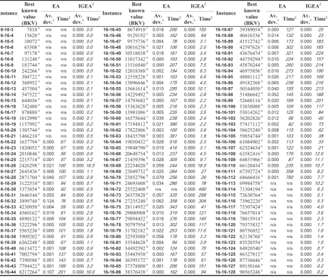
Since our algorithm constantly finds the best known ((pseudo-)optimal) solutions, it is preferable to investigate run time performance instead of solution quality. In such situation, the so-called "time to target" [1] methodology may by used. In this case, for a given target value of the objective function (target solution), the run time of the algorithm to achieve this value is recorded. This is repeated multiple times and the recorded run times are sorted. With each run time, a
probability
w i Pi
5 . 0
is associated, where i (i = 1, 2,
…, w) denotes the number of the current trial and w is the total number of trials (we used w = 10). The probabilities Pi can be visualized using "time-to-tar-get" plots which show the probability that the target value will be obtained (see Figure 10).
0.0 0.1 0.2 0.3 0.4 0.5 0.6 0.7 0.8 0.9 1.0
88 100 128 130 150 160 164 175 190 201
pr
ob
a
bi
li
ty
time (s)
HGA IGEA1 IGEA2
Figure 10. Example of the time-to-target plot for the instance 16-16-90
The performance improvement factor, PIF, of one algorithm (A1) to another one (A2) may be defined by
the following formula:
) A (
) A (
1 5 . 0
2 5 . 0 t t
PIF ; here, t0.5
de-notes the time needed to obtain the target value with probability 0.5. We have compared the performance improvement factors for our improved genetic-evolutionary algorithms (IGEA1, IGEA2) and the previous hybrid genetic algorithm (HGA) presented in [17]. In Table 2, we present, in particular, the values of
t0.5 as well as the values of the performance im-provement factor for HGA, IGEA1 and IGEA2. The values of t0.5 are in seconds. The target values are set to be equal to the corresponding best known values (BKVs). (Only fifty-one instances (from m = 65 to
m= 115) are examined because the remaining problems with m < 65 and m > 115 are, with few ex-ceptions (m = 26, 44, 45, 46), easily solved by all algorithms.)
Table 1. Results of the experiments with the GPP (I)
EA IGEA2 EA IGEA2 EA IGEA2
Instance Best known
value (BKV)
Av. dev.†Time‡
Av. dev.†Time‡
Instance Best known
value (BKV)
Av. dev.† Time‡
Av. dev.† Time‡
Instance Best known
value (BKV)
Av. dev.† Time‡
Av. dev.†Time‡ 16-16-3 7810 a n/a n/a 0.000 0.0 16-16-45 8674910 c 0.018 206 0.000 150 16-16-87 39389054 b 0.000 127 0.000 25 16-16-4 15620 a n/a n/a 0.000 0.0 16-16-46 9129192 c 0.005 162 0.000 64 16-16-88 40416536 b 0.014 132 0.000 23 16-16-5 38072 a n/a n/a 0.000 0.0 16-16-47 9575736 a 0.004 78 0.000 3.1 16-16-89 41512742 b 0.006 173 0.000 183 16-16-6 63508 a n/a n/a 0.000 0.0 16-16-48 10016256 a 0.021 106 0.000 2.0 16-16-90 42597626 e 0.006 302 0.000 165 16-16-7 97178 a n/a n/a 0.000 0.0 16-16-49 10518838 b 0.018 181 0.000 3.4 16-16-91 43676474 e 0.007 321 0.000 224 16-16-8 131240 a n/a n/a 0.000 0.0 16-16-50 11017342 a 0.000 193 0.000 2.8 16-16-92 44759294 g 0.010 224 0.000 157 16-16-9 183744 a n/a n/a 0.000 0.0 16-16-51 11516840 b 0.000 207 0.000 7.5 16-16-93 45870244 e 0.005 260 0.000 214 16-16-10 242266 a n/a n/a 0.000 0.0 16-16-52 12018388 b 0.002 194 0.000 6.3 16-16-94 46975856 e 0.016 273 0.000 190 16-16-11 304722 a n/a n/a 0.000 0.1 16-16-53 12558226 a 0.001 193 0.000 4.6 16-16-95 48081112 h 0.026 217 0.000 169 16-16-12 368952 a n/a n/a 0.000 0.1 16-16-54 13096646 b 0.004 175 0.000 4.0 16-16-96 49182368 a 0.065 236 0.000 216 16-16-13 457504 a n/a n/a 0.000 0.1 16-16-55 13661614 b 0.010 295 0.000 10.1 16-16-97 50344050 a 0.040 155 0.000 213 16-16-14 547522 a n/a n/a 0.000 0.1 16-16-56 14229492 b 0.005 234 0.000 2.8 16-16-98 51486642 a 0.052 145 0.000 188 16-16-15 644036 a n/a n/a 0.000 0.1 16-16-57 14793682 b 0.000 167 0.000 2.2 16-16-99 52660116 a 0.020 169 0.000 201 16-16-16 742480 a n/a n/a 0.000 0.1 16-16-58 15363628 b 0.005 216 0.000 2.3 16-16-100 53838088 a 0.005 109 0.000 117 16-16-17 878888 a n/a n/a 0.000 0.2 16-16-59 15981086 a 0.005 235 0.000 3.5 16-16-101 55014262 a 0.012 125 0.000 84 16-16-18 1012990 a n/a n/a 0.000 0.1 16-16-60 16575644 a 0.039 238 0.000 2.4 16-16-102 56202826 h 0.012 96 0.000 40 16-16-19 1157992 a n/a n/a 0.000 0.2 16-16-61 17194812 b 0.021 386 0.000 2.2 16-16-103 57417112 a 0.002 82 0.000 73 16-16-20 1305744 a n/a n/a 0.000 0.3 16-16-62 17822806 b 0.003 100 0.000 3.6 16-16-104 58625240 h 0.008 115 0.000 62 16-16-21 1466210 a n/a n/a 0.000 0.5 16-16-63 18435790 a 0.003 381 0.000 1.9 16-16-105 59854744 a 0.001 103 0.000 38 16-16-22 1637794 a 0.000 67 0.000 0.3 16-16-64 19050432 a 0.028 516 0.000 2.3 16-16-106 61084902 a 0.002 113 0.000 33 16-16-23 1820052 a 0.000 67 0.000 0.2 16-16-65 19848790 b 0.019 416 0.000 3.1 16-16-107 62324634 a 0.001 122 0.000 21 16-16-24 2010846 a 0.000 56 0.000 0.6 16-16-66 20648754 b 0.013 237 0.000 4.5 16-16-108 63582416 a 0.000 179 0.000 12.6 16-16-25 2215714 b 0.001 97 0.000 3.2 16-16-67 21439396 b 0.028 305 0.000 9.7 16-16-109 64851966 a 0.000 87 0.000 11.1 16-16-26 2426298 c 0.021 100 0.000 16.5 16-16-68 22234020 b 0.059 244 0.000 18.0 16-16-110 66120434 h 0.000 235 0.000 10.7 16-16-27 2645436 a 0.006 100 0.000 1.1 16-16-69 23049732 b 0.025 284 0.000 27 16-16-111 67392724 a 0.000 358 0.000 8.2 16-16-28 2871704 a 0.040 107 0.000 0.9 16-16-70 23852796 b 0.079 256 0.000 26 16-16-112 68666416 a 0.001 790 0.000 7.7 16-16-29 3122510 a 0.001 94 0.000 0.7 16-16-71 24693608 b 0.034 286 0.000 78 16-16-113 69984758 a n/a n/a 0.000 10.2 16-16-30 3373854 a 0.000 92 0.000 0.5 16-16-72 25522408 d n/a n/a 0.000 490 16-16-114 71304194 a n/a n/a 0.000 6.3 16-16-31 3646344 a 0.055 84 0.000 0.6 16-16-73 26375828 e 0.057 335 0.000 298 16-16-115 72630764 a n/a n/a 0.000 5.1 16-16-32 3899744 a 0.124 76 0.000 0.5 16-16-74 27235240 f 0.062 358 0.000 304 16-16-116 73962220 a n/a n/a 0.000 5.3 16-16-33 4230950 a 0.004 59 0.000 0.7 16-16-75 28114952 b 0.020 343 0.000 41 16-16-117 75307424 a n/a n/a 0.000 4.0 16-16-34 4560162 a 0.019 61 0.000 2.6 16-16-76 29000908 b 0.010 319 0.000 121 16-16-118 76657014 a n/a n/a 0.000 3.6 16-16-35 4890132 a 0.006 104 0.000 3.2 16-16-77 29894452 f 0.016 376 0.000 145 16-16-119 78015914 a n/a n/a 0.000 2.3 16-16-36 5222296 a 0.005 105 0.000 2.0 16-16-78 30797954 f 0.013 302 0.000 117 16-16-120 79375832 a n/a n/a 0.000 1.7 16-16-37 5565236 a 0.000 101 0.000 1.8 16-16-79 31702182 b 0.022 253 0.000 11.6 16-16-121 80756852 a n/a n/a 0.000 1.6 16-16-38 5909202 a 0.000 91 0.000 0.9 16-16-80 32593088 b 0.058 178 0.000 3.3 16-16-122 82138768 a n/a n/a 0.000 1.4 16-16-39 6262248 a 0.000 67 0.000 1.1 16-16-81 33544628 b 0.004 94 0.000 3.9 16-16-123 83528554 a n/a n/a 0.000 1.0 16-16-40 6613472 a 0.001 108 0.000 0.9 16-16-82 34492592 b 0.002 124 0.000 70 16-16-124 84920540 a n/a n/a 0.000 0.7 16-16-41 7002794 a 0.001 137 0.000 0.6 16-16-83 35443938 e 0.000 167 0.000 57 16-16-125 86327812 a n/a n/a 0.000 0.4 16-16-42 7390586 a 0.001 143 0.000 0.7 16-16-84 36395172 e 0.001 178 0.000 61 16-16-126 87736646 a n/a n/a 0.000 0.3 16-16-43 7794422 b 0.001 199 0.000 3.2 16-16-85 37378800 e 0.001 206 0.000 151 16-16-127 89150166 a n/a n/a 0.000 0.2 16-16-44 8217264 b 0.107 201 0.000 16.0 16-16-86 38376438 c 0.000 162 0.000 94 16-16-128 90565248 a n/a n/a 0.000 0.2
† the average deviation (Av. dev.) is measured in percentage of average solution over BKV; ‡ times for EA and IGEA2 are given in seconds per run for 2.8 GHz and 3 GHz computers, respectively;
a comes from [30]; b comes from [14]; c comes from [13]; d comes from this paper; e comes from [5,17]; f comes from [15]; g comes from [27]; h comes from [16]
Table 2. Results of the experiments with the GPP (II)
Instance t0.5 t0.5 t0.5¡ PIF1PIF2PIF3Instance t0.5 t0.5 t0.5¡ PIF1PIF2PIF3 Instance t0.5 t0.5 t0.5¡ PIF1PIF2PIF3
16-16-65 2.9 2.9 2.4 1.00 1.21 1.21 16-16-82 61.1 59.0 51.4 1.04 1.19 1.15 16-16-99 194.0 172.0 162.0 1.13 1.20 1.06
16-16-66 4.7 3.5 3.2 1.34 1.47 1.09 16-16-83 55.4 47.4 48.0 1.17 1.15 0.99 16-16-100 110.1 99.0 101.4 1.11 1.09 0.98
16-16-67 9.3 9.0 6.7 1.03 1.39 1.34 16-16-84 61.0 52.2 49.5 1.17 1.23 1.05 16-16-101 94.0 77.3 81.0 1.22 1.16 0.95
16-16-68 19.3 16.0 12.3 1.21 1.57 1.30 16-16-85 132.6 131.8 110.3 1.01 1.20 1.19 16-16-102 36.9 37.0 34.9 1.00 1.06 1.06
16-16-69 28.1 23.8 15.6 1.18 1.80 1.53 16-16-86 93.8 93.8 70.1 1.00 1.34 1.34 16-16-103 74.5 66.4 52.8 1.12 1.41 1.26
16-16-70 26.6 22.4 21.4 1.19 1.24 1.05 16-16-87 20.9 18.1 16.1 1.15 1.30 1.12 16-16-104 68.5 59.3 50.0 1.16 1.37 1.19
16-16-71 82.8 67.5 56.3 1.23 1.47 1.20 16-16-88 25.2 23.5 20.5 1.07 1.23 1.15 16-16-105 43.8 32.9 32.4 1.33 1.35 1.02
16-16-72 n/a 597.0 450.0 n/a n/a 1.33 16-16-89 172.0 163.0 140.1 1.06 1.23 1.16 16-16-106 34.0 32.7 25.0 1.04 1.36 1.31
16-16-73 330.0 263.2 285.0 1.26 1.16 0.92 16-16-90 191.3 160.7 127.0 1.19 1.51 1.27 16-16-107 20.4 14.0 16.0 1.46 1.28 0.88
16-16-74 284.7 280.0 227.0 1.02 1.25 1.23 16-16-91 246.0 189.8 171.0 1.30 1.43 1.10 16-16-108 12.6 10.8 10.6 1.17 1.19 1.02
16-16-75 49.7 40.2 33.5 1.24 1.48 1.20 16-16-92 172.8 156.0 132.6 1.11 1.30 1.18 16-16-109 11.1 9.4 8.2 1.18 1.35 1.15
16-16-76 109.3 105.4 96.0 1.04 1.14 1.10 16-16-93 267.7 195.1 203.5 1.37 1.32 0.96 16-16-110 11.2 11.0 8.1 1.02 1.38 1.36
16-16-77 149.0 136.0 124.3 1.10 1.20 1.09 16-16-94 196.9 150.0 170.9 1.31 1.15 0.88 16-16-111 8.2 8.1 6.2 1.01 1.32 1.31
16-16-78 98.7 96.7 88.9 1.02 1.11 1.09 16-16-95 216.0 145.1 150.0 1.49 1.44 0.97 16-16-112 7.3 6.2 5.9 1.18 1.24 1.05
16-16-79 12.3 10.4 8.0 1.18 1.54 1.30 16-16-96 239.8 215.1 157.0 1.11 1.53 1.37 16-16-113 10.1 7.9 6.4 1.28 1.58 1.23
16-16-80 3.5 3.1 3.1 1.13 1.13 1.00 16-16-97 216.7 211.0 180.2 1.03 1.20 1.17 16-16-114 6.5 4.9 4.1 1.33 1.59 1.20
16-16-81 3.7 3.3 3.0 1.12 1.23 1.10 16-16-98 190.0 180.4 134.5 1.05 1.41 1.34 16-16-115 4.7 4.1 3.8 1.15 1.24 1.08
Average: --- 1.16 1.32 1.15
Notes: t0.5 = t0.5(HGA), t0.5 = t0.5(IGEA1), t0.5¡ = t0.5(IGEA2),
) IGEA (
) HGA (
1 5 . 0 5 . 0 1
t t
PIF ,
) IGEA (
) HGA (
2 5 . 0 5 . 0 2
t t
PIF ,
) IGEA (
) IGEA (
2 5 . 0
1 5 . 0 3
Table 3. Results of the experiments with the GPP (III)
Instance t0.5 t0.5 t0.5 PIF4PIF5PIF6Instance t0.5 t0.5 t0.5 PIF4PIF5PIF6 Instance t0.5 t0.5 t0.5 PIF4PIF5PIF6
16-16-65 1.8 1.2 0.2 1.50 9.00 6.00 16-16-8239.4 26.1 3.9 1.51 10.10 6.69 16-16-99 124.1 77.1 12.0 1.61 10.34 6.43
16-16-66 2.8 1.6 0.2 1.75 14.00 8.00 16-16-8335.0 20.9 3.6 1.67 9.72 5.81 16-16-100 67.7 44.1 7.5 1.54 9.03 5.88
16-16-67 5.7 3.9 0.5 1.46 11.40 7.80 16-16-8437.2 23.4 3.7 1.59 10.05 6.32 16-16-101 58.0 32.8 6.1 1.77 9.51 5.38
16-16-68 12.1 7.0 0.9 1.73 13.44 7.78 16-16-8583.2 58.9 8.3 1.41 10.02 7.10 16-16-102 23.6 15.9 2.6 1.48 9.08 6.12
16-16-69 17.7 10.7 1.2 1.65 14.75 8.92 16-16-8656.3 40.8 5.3 1.38 10.62 7.70 16-16-103 47.7 29.1 3.9 1.64 12.23 7.46
16-16-70 16.1 9.4 1.6 1.71 10.06 5.88 16-16-8712.7 8.1 1.2 1.57 10.58 6.75 16-16-104 41.9 25.5 3.7 1.64 11.32 6.89
16-16-71 52.9 29.7 4.2 1.78 12.60 7.07 16-16-8815.9 10.0 1.5 1.59 10.60 6.67 16-16-105 27.1 14.6 2.4 1.86 11.29 6.08
16-16-72 451.9 262.0 33.2 1.72 13.61 7.89 16-16-89106.2 72.3 10.5 1.47 10.11 6.89 16-16-106 21.6 14.5 1.8 1.49 12.00 8.06
16-16-73 210.4 115.0 21.5 1.83 9.79 5.35 16-16-90116.9 67.5 9.4 1.73 12.44 7.18 16-16-107 12.8 6.0 1.2 2.13 10.67 5.00
16-16-74 171.2 118.0 17.0 1.45 10.07 6.94 16-16-91155.7 84.6 12.9 1.84 12.07 6.56 16-16-108 7.6 4.8 0.8 1.58 9.50 6.00
16-16-75 31.2 16.9 2.5 1.85 12.48 6.76 16-16-92110.5 67.1 9.8 1.65 11.28 6.85 16-16-109 6.7 4.1 0.6 1.63 11.17 6.83
16-16-76 68.0 46.5 7.2 1.46 9.44 6.46 16-16-93169.9 88.1 15.0 1.93 11.33 5.87 16-16-110 6.8 4.7 0.6 1.45 11.33 7.83
16-16-77 91.1 60.0 9.3 1.52 9.80 6.45 16-16-94121.2 66.2 12.8 1.83 9.47 5.17 16-16-111 5.2 3.5 0.5 1.49 10.40 7.00
16-16-78 63.3 41.2 6.6 1.54 9.59 6.24 16-16-95131.1 63.9 11.1 2.05 11.81 5.76 16-16-112 4.4 2.7 0.4 1.63 11.00 6.75
16-16-79 7.8 4.4 0.6 1.77 13.00 7.33 16-16-96153.9 95.1 11.7 1.62 13.15 8.13 16-16-113 6.3 3.5 0.5 1.80 12.60 7.00
16-16-80 2.2 1.3 0.2 1.69 11.00 6.50 16-16-97132.2 95.2 13.3 1.39 9.94 7.16 16-16-114 4.0 2.2 0.3 1.82 13.33 7.33
16-16-81 2.3 1.4 0.2 1.64 11.50 7.00 16-16-98122.4 79.7 10.1 1.54 12.12 7.89 16-16-115 2.9 1.7 0.3 1.71 9.67 5.67
Average: --- 1.65 11.09 6.76
Notes: t0.5 = t0.5(SD), t0.5 = t0.5(SA), t0.5 = t0.5(IGEA2),
) SA (
) SD (
5 . 0 5 . 0 4
t t
PIF ,
) IGEA (
) SD (
2 5 . 0
5 . 0 5
t t
PIF ,
) IGEA (
) SA (
2 5 . 0
5 . 0 6
t t PIF
Table 4. Results of the experiments with the GPP (IV)
Instance t0.5 t0.5 t0.5 PIF7PIF8PIF9Instance t0.5 t0.5 t0.5 PIF7PIF8PIF9 Instance t0.5 t0.5 t0.5 PIF7PIF8PIF9
16-16-65 0.6 0.4 0.2 1.50 3.00 2.00 16-16-8212.3 7.7 3.9 1.60 3.15 1.97 16-16-99 41.0 21.0 12.0 1.95 3.42 1.75
16-16-66 1.0 0.4 0.2 2.50 5.00 2.00 16-16-8311.2 5.9 3.6 1.90 3.11 1.64 16-16-100 23.2 13.0 7.5 1.78 3.09 1.73
16-16-67 1.9 1.1 0.5 1.73 3.80 2.20 16-16-8412.4 6.6 3.7 1.88 3.35 1.78 16-16-101 18.7 10.1 6.1 1.85 3.07 1.66
16-16-68 3.8 2.1 0.9 1.81 4.22 2.33 16-16-8527.3 17.3 8.3 1.58 3.29 2.08 16-16-102 7.8 4.6 2.6 1.70 3.00 1.77
16-16-69 5.7 3.1 1.2 1.84 4.75 2.58 16-16-8619.8 11.5 5.3 1.72 3.74 2.17 16-16-103 15.0 8.5 3.9 1.76 3.85 2.18
16-16-70 5.5 2.9 1.6 1.90 3.44 1.81 16-16-87 4.3 2.3 1.2 1.87 3.58 1.92 16-16-104 13.7 7.5 3.7 1.83 3.70 2.03
16-16-71 16.8 9.0 4.2 1.87 4.00 2.14 16-16-88 5.3 2.9 1.5 1.83 3.53 1.93 16-16-105 8.9 4.0 2.4 2.23 3.71 1.67
16-16-72 141.1 74.1 33.2 1.90 4.25 2.23 16-16-8934.5 21.4 10.5 1.61 3.29 2.04 16-16-106 7.0 4.2 1.8 1.67 3.89 2.33
16-16-73 69.4 33.9 21.5 2.05 3.23 1.58 16-16-9038.9 21.1 9.4 1.84 4.14 2.24 16-16-107 4.0 1.8 1.2 2.22 3.33 1.50
16-16-74 57.4 36.4 17.0 1.58 3.38 2.14 16-16-9151.9 25.2 12.9 2.06 4.02 1.95 16-16-108 2.6 1.4 0.8 1.86 3.25 1.75
16-16-75 9.9 5.1 2.5 1.94 3.96 2.04 16-16-9235.6 20.4 9.8 1.75 3.63 2.08 16-16-109 2.3 1.2 0.6 1.92 3.83 2.00
16-16-76 22.1 13.4 7.2 1.65 3.07 1.86 16-16-9353.5 24.9 15.0 2.15 3.57 1.66 16-16-110 2.4 1.4 0.6 1.71 4.00 2.33
16-16-77 29.8 17.9 9.3 1.66 3.20 1.92 16-16-9439.0 19.0 12.8 2.05 3.05 1.48 16-16-111 1.7 1.1 0.5 1.55 3.40 2.20
16-16-78 20.0 12.0 6.6 1.67 3.03 1.82 16-16-9542.9 17.8 11.1 2.41 3.86 1.60 16-16-112 1.5 0.8 0.4 1.88 3.75 2.00
16-16-79 2.6 1.3 0.6 2.00 4.33 2.17 16-16-9649.2 27.8 11.7 1.77 4.21 2.38 16-16-113 2.1 1.0 0.5 2.10 4.20 2.00
16-16-80 0.7 0.4 0.2 1.75 3.50 2.00 16-16-9743.0 27.9 13.3 1.54 3.23 2.10 16-16-114 1.4 0.6 0.3 2.33 4.67 2.00
16-16-81 0.8 0.4 0.2 2.00 4.00 2.00 16-16-9840.2 22.9 10.1 1.76 3.98 2.27 16-16-115 1.0 0.5 0.3 2.00 3.33 1.67
Average: --- 1.86 3.65 1.97
Notes: t0.5 = t0.5(TS), t0.5 = t0.5(GA-SD), t0.5 = t0.5(IGEA2),
SD)
(GA-) TS (
5 . 0
5 . 0 7
t t
PIF ,
) IGEA (
) TS (
2 5 . 0
5 . 0 8
t t
PIF ,
) IGEA (
SD)
(GA-2 5 . 0 5 . 0 9
t t PIF
Table 5. New best known solution for the GPP
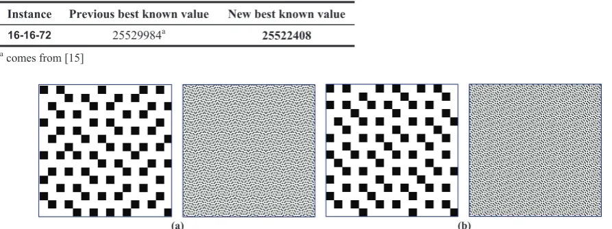
Instance Previous best known value New best known value
16-16-72 25529984a 25522408
a comes from [15]
Figure 11. Previous (a) and new (b) best known grey frames of density 72/256: larger- and smaller-scale views
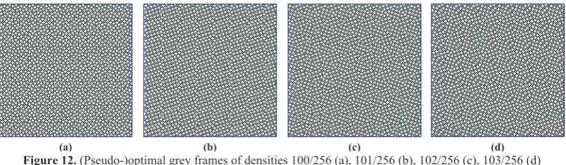
Figure 12. (Pseudo-)optimal grey frames of densities 100/256 (a), 101/256 (b), 102/256 (c), 103/256 (d)
We have also compared the algorithm IGEA2 with other well-known algorithms, in particular, steepest descent (SD) algorithm, simulated annealing (SA) algorithm, tabu search (TS) algorithm, and genetic (evolutionary) algorithm hybridized with steepest descent (GA-SD). All these algorithms were coded and implemented by the author; the descriptions of the algorithms can be found in [5]. The results of the comparison of the algorithms are presented in Tables 3 and 4. Similarly to Table 2, we present the values of
t0.5 and PIF. The values of t0.5 are again in seconds, however the target values are 0.1% above BKVs.
Note that during the experiments, we were successful in discovering new record-breaking solution for the instance 16-16-72 (m = 72) (see Table 5). As a confirmation of the quality of the solution produced, we give the visual representation of this solution and the previous best known solution in Figure 11. Some other (pseudo-)optimal grey frames are shown in Figure 12 so that the reader can judge about the excellence of the grey patterns generated.
4. Conclusions
In this work, the issues related to solving the grey pattern problem (GPP) are discussed. We propose to use an improved genetic-evolutionary algorithm (IGEA), which is based on the integrating of intensi-fication and diversiintensi-fication (I&D) approaches. The main improvements of IGEA are due the special recombination of solutions and the enhanced intra-evolutionary procedure as a post-recombination algo-rithm. The recombination has both diversification and intensification effect. The post-recombination algo-rithm itself consists of the iterative tabu search and mutation processes, where the tabu search serves as a basic intensification mechanism. The fast descent and extended decent-based local search procedures are designed to play the role of alternative intensification. The specialized mutation operator has exclusively diversification effect.
The new results from the experiments show promising performance of the proposed algorithm, as well as its superiority to the previous efficient hybrid genetic algorithm proposed in [17]. These results sup-port the opinion that is extremely imsup-portant to use a smart post-recombination procedure as well as a proper mechanism for premature convergence
avoidance. It is confirmed that integrating I&D into the evolutionary process has a quite remarkable effect on the quality of solutions.
The effectiveness of our algorithm is also corro-borated by the fact that all GPP instances are solved to pseudo-optimality at surprisingly small computational effort. The new best known grey pattern of density 72/256 has been discovered.
Acknowledgments
The author thanks anonymous referees for the valuable comments and suggestions that contributed to significantly improve the quality of the paper.
References
[1] R.M. Aiex, M.G.C. Resende, C.C. Ribeiro. Prob-ability distribution of solution time in GRASP: An experimental investigation. Journal of Heuristics, 2002, Vol.8, 343–373.
[2] T. Bäck, D.B. Fogel, Z. Michalewicz (eds). Handbook of Evolutionary Computation. Institute of Physics Publishing, Bristol, 1997.
[3] O. Berman, Z. Drezner. The multiple server location problem. Journal of Operational Research Society, 2007, Vol.58, 91–99.
[4] R.E. Burkard, E. Çela, P.M. Pardalos, L. Pitsoulis. The quadratic assignment problem. In D.Z.Du, P.M. Pardalos (eds.), Handbook of Combinatorial Optimi-zation, Kluwer, Dordrecht, 1998, Vol.3, 241–337. [5] Z. Drezner. Finding a cluster of points and the grey
pattern quadratic assignment problem. OR Spectrum, 2006, Vol.28, 417436.
[6] C. Fleurent, J.A. Ferland. Genetic hybrids for the quadratic assignment problem. In P.M.Pardalos, H. Wolkowicz (eds.), Quadratic Assignment and Related Problems. DIMACS Series in Discrete Mathematics and Theoretical Computer Science, Vol.16, AMS, Pro-vidence, 1994, 173188.
[7] F. Glover, M. Laguna. Tabu search. Kluwer, Dord-recht, 1997.
[8] D.E. Goldberg. Genetic Algorithms in Search, Opti-mization and Machine Learning. Addison-Wesley, Reading, 1989.
[9] A. Hertz, D. Kobler. A framework for the description of evolutionary algorithms. European Journal of Operational Research, 2000, Vol.126, 112.
[10] J.H.Holland. Adaptation in Natural and Artificial Systems. University of Michigan Press, Ann Arbor, 1975.
[11] E.L. Lawler. The quadratic assignment problem. Ma-nagement Science, 1963, Vol.9, 586599.
[12] Z. Michalewicz, D.B. Fogel. How to Solve It: Modern Heuristics. Springer, Berlin-Heidelberg, 2000. [13] A. Misevicius. Genetic algorithm hybridized with ruin
and recreate procedure: application to the quadratic assignment problem. Knowledge-Based Systems, 2003, Vol.16, 261268.
[14] A. Misevicius. Ruin and recreate principle based approach for the quadratic assignment problem. In E.Cantú-Paz, J.A.Foster, K.Deb et al. (eds.), Lecture Notes in Computer Science, Vol. 2723: Genetic and Evolutionary Computation — GECCO 2003, Procee-dings, Part I, Springer, Berlin-Heidelberg-New York, 2003, 598609.
[15] A. Misevicius. An improved hybrid genetic algorithm: new results for the quadratic assignment problem. Knowledge-Based Systems, 2004, Vol.17, 6573. [16] A. Misevicius. A tabu search algorithm for the
quad-ratic assignment problem. Computational Optimiza-tion and ApplicaOptimiza-tions, 2005, Vol.30, 95111.
[17] A. Miseviius. Experiments with hybrid genetic algo-rithm for the grey pattern problem. Informatica, 2006, Vol.17, 237258.
[18] A. Miseviius. Testing of crossover operators for the grey pattern problem. kio technologinis ir ekonomi-nis vystymas (Technological and Economic Develop-ment of Economy), 2006, Vol.17, 3743.
[19] A. Miseviius. Experiments with local search heuris-tics for the traveling salesman problem. In A. Targa-madz, R. Butleris, R. Butkien (eds.), Proceedings of the 16th International Conference on Information and Software Technologies, IT-2010, Technologija, Kau-nas, 2010, 4753.
[20] A. Miseviius, A. Lenkeviius, D. Rubliauskas. Iterated tabu search: an improvement to standard tabu search. Information Technology and Control, 2006, Vol.35, 187197.
[21] A. Miseviius, D. Rubliauskas. Enhanced improve-ment of individuals in genetic algorithms. Information Technology and Control, 2008, Vol.37, No.3, 179186.
[22] A.Miseviius, D.Rubliauskas, V.Barkauskas. Some further experiments with the genetic algorithm for the quadratic assignment problem. Information Technology and Control, 2009, Vol.38, No.4, 325332.
[23] P. Moscato. Memetic algorithms: a short introduction. In D. Corne, M. Dorigo, F.Glover (eds.), New Ideas in Optimization, 1999, McGraw-Hill, London, 219234. [24] V. Nissen. Solving the quadratic assignment problem
with clues from nature. IEEE Transactions on Neural Networks, 1994, Vol.5, 6672.
[25] I. Rechenberg. Evolutionsstrategie: Optimierung Technischer Systeme nach Prinzipien der Biologi-schen Evolution. Formann-Holzboog Verlag, Stutt-gart, 1973.
[26] H.-P. Schwefel. Evolutionsstrategie und numerische Optimierung. PhD Thesis, Technische Universität Berlin, Germany, 1975.
[27] T. Stützle. MAX-MIN ant system for quadratic assignment problems. Res. Report AIDA-97-04, Darm-stadt University of Technology, Germany, 1997. [28] G. Syswerda. Uniform crossover in genetic
algo-rithms. In J.D. Schaffer (ed.), Proceedings of the Third International Conference on Genetic Algorithms, 1989, Morgan Kaufmann, San Mateo, 29.
[29] E. Taillard. Comparison of iterative searches for the quadratic assignment problem. Location Science, 1995, Vol.3, 87105.
[30] E. Taillard, L.M. Gambardella. Adaptive memories for the quadratic assignment problem. Tech. Report IDSIA-87-97, Lugano, Switzerland, 1997.
[31] D.M. Tate, A.E. Smith. A genetic approach to the quadratic assignment problem. Computers & Opera-tions Research, 1995, Vol.1, 7383.
Appendix
Figure A1. Pseudo-code of the fast randomized tabu search algorithm. Notes. 1. The function if(x,y1,y2) returns y1 if x = TRUE, otherwise it returns y2. 2. The function random() returns a pseudo-random number uniformly distributed in [0, 1]
Figure A2. Pseudo-code of the fast steepest descent algorithm using the neighbourhood 12
procedure FastRandomizedTabuSearch;
// input: S current solution, n problem size, m # of black points, B distance matrix,
// hmin, hmax lower and higher tabu tenures, W # of iterations, Z alternative intensification period, D randomization level // output: Sx the best solution found
for i := 1 to StackHeader do Tabu[Stack1[i], Stack2[i]] := 0;// tabu list initialization
for i := 1 to n do begin ci := 0; for j := 1 to m do ci := ci + biS(j) end; // initialization of C Sx := S; k := 1; kc := 1; improved := FALSE; choose h randomly between h
min and hmax;
while (kdW) or (improved = TRUE) then begin // main cycle
'min := f;
for i := 1 to m do // m(nm) neighbours of S are considered
for j := m + 1 to n do begin
' := 2(cS(j)cS(i)bS(i)S(j));
forbidden := if((Tabu[i,j] tk) and (random() tD), TRUE, FALSE); aspired := if((z(S) + ' < z(Sx)) and forbidden), TRUE, FALSE);
if ((' < 'min) andnot(forbidden)) oraspiredthenbegin'min := ';u := i;v := jend
end; // for
if 'min < f then begin
S
S: puv; for i := 1 to n do ci := ci + biS(u)biS(v); // replace the current solution by the new one and update C
Tabu[u,v] := k + h; // update tabu list (make the move puv tabu)
StackHeader := StackHeader+ 1;Stack1[StackHeader] := u;Stack2[StackHeader] := v
end; // if
improved := if('min < 0, TRUE, FALSE);
if improved and (kkctZ) then begin // switch to alternative intensification (depending on the version of IGEA)
apply FastSteepestDescent | FastExtendedSteepestDescent to S; kc := k
end;
if z(S) < z(Sx) then Sx := S; // save the best so far solution
k := k + 1
end // while
end.
procedure FastSteepestDescent;
// input: S current solution, n problem size, m # of black points, B distance matrix // output: S resulting (improved) solution
for i := 1 to n do begin ci := 0; for j := 1 to m do ci := ci + biS(j) end;
repeat // cycle is repeated until local optimum is reached
'min := 0;
for i := 1 to m do
for j := m + 1 to n do begin ' := 2(cS(j)cS(i)bS(i)S(j));if ' < 'minthenbegin'min := ';u := i;v := jend end;
if 'min < 0 then begin // replace the current solution by the better one
S
S: puv; for i := 1 to n do ci := ci + biS(u)biS(v)
end // if
until 'mint 0