S. Descombes, B. Dussoubs, S. Faure, L. Gouarin, V. Louvet, M. Massot, V. Miele, Editors
PARALLELIZATION OF A RELAXATION SCHEME MODELLING THE
BEDLOAD TRANSPORT OF SEDIMENTS IN SHALLOW WATER FLOW
E. Audusse
1, O. Delestre
2, M. H. Le
3, M. Masson-Fauchier
4, P. Navaro
5et
R. Serra
6R´esum´e. Nous nous int´eressons dans ce travail `a la simulation num´erique des processus d’´erosion par charriage en rivi`ere. Nous pr´esentons un sch´ema num´erique bas´e sur un mod`ele de relaxation et nous l’appliquons `a des probl`emes de d´eplacement de dunes en une et deux dimensions d’espace. Nous ´etudions en particulier les ph´enom`enes d’antidune pr´esent´es dans la litt´erature hydros´edimentaire. Nous pr´esentons enfin une proc´edure de parall´elisation bas´ee sur l’utilisation de la librairie MPI et qui nous permet de simuler des processus bidimensionnels avec des temps CPU raisonnables.
Abstract. In this work we are interested in numerical simulations for bedload erosion processes. We present a relaxation solver that we apply to moving dunes test cases in one and two dimensions. In particular we retrieve the so-called anti-dune process that is well described in the experiments. In order to be able to run 2D test cases with reasonable CPU time, we also describe and apply a parallelization procedure by using domain decomposition based on the classical MPI library.
1.
Introduction
Soil erosion is a complex phenomenon affected by many factors such as climate, topography, soil characteris-tics, vegetation and anthropogenic activities such as cultivation practices. Erosion process can be described in three stages: detachment, transport and deposition. The detachment occurs when the flow shear stress or the kinetic energy of raindrop exceeds the cohesive strength of the soil particles. Once detached, the sediments can be transported downstream as non-cohesive sediment before its deposition.
The movement of sediments occurs in two main modes called bedload and suspended load. The bedload particles are located in a few grain diameters thick layer situated on the soil. The velocities of these particles are less than the flow velocity. At the opposite, the suspended particles are transported in the flow without contact with the bed. Sediments finer than 0.2 mm which are transported in suspension are rarely included/considered in bedload. The distinction between these two modes of sediment transport is blurred because they occur together.
As soil erosion by water continues to be a serious problem throughout the world, the development of improved soil erosion prediction technology is required. With the increase of computing powers in the last years, there has
1BANG Project, INRIA-Paris-Rocquencourt & LAGA, Universiy Paris 13 Nord, France, e-mail : [email protected] 2 Lab. J.A. Dieudonn´e & EPU Nice Sophia, University of Nice, France, e-mail : [email protected]
3 MAPMO, University of Orl´eans, France, e-mail : [email protected] 4 EPU Nice Sophia, University of Nice, France
5 IRMA, UMR 7501 CNRS, Unistra, France, e-mail : [email protected] 6 EPU Nice Sophia, University of Nice, France
c
EDP Sciences, SMAI 2013
been a rapid increase in the erosion and sediment transport simulations through the use of computer models. The models describing erosion process are available at different level of complexity. In general, erosion process is described by the equations of evolution based on the principle of conservation. These equations are derived at small scale under physical assumptions.
2.
Bedload modelling
In this paper, we focus on the modelling of the morphodynamic process where the solid transport is only characterized by bedload and thus the suspended load has been ignored. The governing equations are often given by coupling the shallow water equations, describing the flow routing [34], with the Exner equation [32] expressing the mass conservation of sediment layer. The one-dimensional system may be written in the form
∂th+∂x(hu) = 0,
∂t(hu) +∂x(hu2+gh2/2) =
−gh∂xzb, ∂tzb+∂xqb= 0,
(1)
where his the water depth, u the flow velocity, zb the thickness of sediment layer, qb the volumetric bedload sediment transport rate per unit time and width andg the acceleration due to gravity.
The expression of bedload flux qb is necessary to close the model (1). Many researches have developed different empirical formulæ to predict and to estimate qb. One of the simplest expression was proposed by Grass [35] whereqbis a function of the flow velocity and a dimensionalAgconstant, called interaction constant, that encompasses the effects of grain size and kinematic viscosity and is usually determined from experimental data:
qb =Agu|u|mg−1, 1
≤mg≤4. (2)
The usual value of the exponentmgis set tomg= 3. IfAg= 0 then we have a solid bed (no sediment transport) and we recover the standard shallow water equations. WhenAgis near zero, there is a small interaction between the fluid and the bed, while ifAg is near one the interaction is larger. Note that one of the main characteristics of this model is that threshold value to initiate the motion of sediment is set to zero, so the sediment transport begins at the same instant that beginning fluid motion.
In practice, qb is usually represented under the non-dimensional form qb∗ as a function of the dimensionless
shear stressτb∗and a threshold valueτcr∗,i.e.
qb =qb∗ p
(s−1)gd3
s, qb∗=qb∗(τb∗, τcr∗), τb∗= τb
(ρs−ρ)gds,
where τb = ρghSf is the bottom shear stress, i.e. the force of water acting on the bed during its routing,
s=ρs/ρthe density relative of sediment in water anddsthe average value of sediment diameters. The friction termSf can be quantified by different empirical laws such as the Darcy-Weisbach or Manning formulæ,i.e.
• Darcy-Weisbach: Sf = f u8gh|u|,
• Manning: Sf =nh2u|u|4/3 ,
where f and n are the Darcy-Weisbach and the Manning coefficients respectively. The threshold value τcr∗
The followings expressions, illustrated by Fig. 1, have been often applied [13, 54, 55, 57]:
Meyer-Peter & M¨uller (1948): qb∗= 8(τb∗−τcr∗) 3/2
+ (3)
Fern´andez Luque & Van Beek (1976): qb∗= 5.7(τb∗−τcr∗)3+/2 (4)
Nielsen (1992): q∗b = 12 p
τ∗
b(τb∗−τcr∗)+ (5)
Ribberink (1998): q∗b = 11(τb∗−τcr∗)1+.65 (6)
Camenen and Larson (2005): q∗b = 12(τb∗)1.5exp (−4.5τcr∗/τb∗) (7)
0.001
0.01
0.1
1
10
0.01
0.1
1
q
∗ b
τ
b∗Meyer-Peter and Muller (1948) Bagnold (1956)
Yalin (1963)
Fernandez Luque and Van Beek (1976) Engelund and Fredsoe (1976)
Parker (1979) Nielsen (1992) Ribberink (1998) Cheng (2002)
Camenen and Larson (2005)
Figure 1. Plot of several bedload functions found in the literature [33],τcr∗ = 0.05.
Upon initiation of flow routing, the topographyzb becomes unstable resulting the fluid-sediment interaction. Various bedforms can be occurred, in particular the formation ofripples, dunesandanti-dunes(see e.g. [46, 47]). Ripples are distinguished from dunes by their much smaller scale. Indeed, ripples and dunes often co-exist, with ripples forming on the larger dunes. At very low flow rates, ripples form on the bed, and as the flow rate increases, these are replaced by the longer wavelength and larger amplitude dunes which migrate slowly downstream. Ripples and dunes are observed in fluvial regime (the Froude numberF r < 1). When the flow becomes supercritical (F r >1), dunes migrate upstream and called anti-dunes.
Let us show quickly how dunes and anti-dunes can be reproduced by the non-linear coupled system (1) (see [23] for more details). Rewriting the system in quasi-linear form as
∂tW+A(W)∂xW = 0
whereW = (h, hu, zb) andA(W) the matrix of transport coefficients being
A(W) =
0 1 0
gh−u2 2u gh
α β 0
withα= ∂qb
∂h and β= ∂qb
∂hu. In [23], we can find two type of relations betweenαandβ for different formulas
ofqb (equations (2)-(7)) which depend on the friction laws:
• with Darcy-Weisbach’s law: α=−uβ,
Moreover, it is natural to assume that β >0 since sediment rate increases with that of flow. The characteristic polynomial ofA(W) can be written as
pA(λ) =−λ[(u−λ)2
−gh)] +gh(βλ+α) =−(λ−λ1)(λ−λ2)(λ−λ3),
whereλ1, λ2, λ3represent the waves speeds propagation of the current and sediment transport. The product
of these eigenvalues, in the caseu >0 (soα >0), satisfies
λ1λ2λ3=pA(0) =ghα <0.
This means that there exists at least a negative eigenvalue. In a sub-critical flow (F r <1), one wave speed of the current is negative and the other one is positive. So the wave speed relating to sediment transport is positive and consequently the dune migrates downstream. Contrary, when the flow becomes supercritical (F r >1), two waves speed of the current are positive and the wave corresponding to sediment transport propagates upstream so we have anti-dune.
System (1) with closed laws (2-7) of qb has recently been proved to be hyperbolic within the range of flow data typical of practical situations [23, 50]. Moreover, numerical approximations of such system are often based on a splitting method, solving first shallow water equations on a time step and updating afterwards the topography using the Exner equation. It is shown that this strategy can create spurious/unphysical oscillations. By contrast, a numerical method that solves the whole system at once will be called a coupled approach in the following.
This paper is organized as follows: in next section, we describe a relaxation approach of the coupled system (1) and we derive a numerical solver. Next, we describe the parallelization procedure we apply in order to run 2D test cases. Finally we present numerical test cases for moving dunes in one and two dimensions, including so-called anti-dune process.
3.
Numerical method
In this work we want to investigate a coupled approach to numerically solve the 1D and 2D SW-Exner system. Such methods were already proposed in the last decade, mostly by considering extension of classical methods to non-conservative systems : Hudson et al. [42] and Castro et al. [18] use a non-conservative Roe scheme based on the theory of paths, see [24] ; Benkhaldoun et al. [5] apply the SRNH scheme whereas Canestrelli et al. [15] introduce the PRICE-R scheme, that is the extension to non-conservative systems of the so-called FORCE scheme. In [4, 16, 19], 2D versions of the preceding works are presented. Other authors also present 2D numerical schemes based on approximate Riemann solvers as extension of HLLC scheme [52, 56, 61]. In [9], the authors present an implicit procedure using the solvers presented in [5, 18].
Here we apply a relaxation solver to find approximate solutions of (1). The relaxation framework for the SW-Exner model was introduced and analysed in [3]. Note that a first relaxation model for SW-SW-Exner model was introduced in [27] but it slightly differs from the model that we are using in this work since it is very generic and it does not use the particular form of the SW-Exner system in its definition. A relaxation solver is a particular approximate Riemann solver where the linearization is introduced in the definition of the relaxation model. By comparison to other types of approximate Riemann solvers, the relaxation framework presents some advantages since it is possible to ensure the positivity of the water height and to prove discrete energy estimates. Moreover the relaxation approach does not need a precise computation of the eigenvalues of the original system and it can be applied to conservative and non-conservative systems. The main idea if the relaxation framework is to replace the fully non-linear system (1) by an enlarged relaxation model that involves two types of parameters (called relaxation parameter and wave celerity parameters) and that satisfies the following properties
• The relaxation model is stable under some bounds on the wave celerity parameters.
• The hyperbolic part of the relaxation system is linearly degenerate.
• The related Riemann problem can be analytically solve in a (quite) easy way.
Starting from the numerical approximation at timetn, the numerical procedure is then very simple : first the
auxiliary quantities are computed by using the physical quantities at time tn, then a homogeneous Riemann
problem is solved at each interface on time step [tn, tn+1] and the new physical quantities at time tn+1 are
computed by considering the mean value of the solution of these Riemann problems on each cell.
The particular relaxation system that we consider in this work stands
∂H ∂t +
∂Hu
∂x = 0 (8)
∂Hu ∂t + ∂ ∂x Hu 2 + Π
+gH∂Z
∂x = 0 (9)
∂Π
∂t +u ∂Π ∂x + a2 H ∂u ∂x = 1 λ( gH2
2 −Π) (10)
∂Z ∂t +
∂Ω
∂x = 0 (11)
∂Ω
∂t + b2
H2 −u 2
∂Z
∂x + 2u ∂Ω
∂x =
1
λ(Qs−Ω) (12)
where Π and Ω are the auxiliary quantities (associated to fluid pressure and to sediment flux, respectively),λ
is the relaxation parameter anda andb are wave celerity parameters. The detailed analysis of this relaxation model and the derivation of the related relaxation scheme have been performed in [3]. Let us recall some important points
• The ”fluid” part of the relaxation model (8)-(12), i.e. the three first equations, is nothing but the so-called Suliciu relaxation model for the classical shallow water system. The ”solid” part of the relaxation model (8)-(12), i.e. the two last equations, is a classical relaxation model for a scalar conservation law and the coefficients are chossen in order to retrieve wave celerities that are centered around the water velocityu.
• The stability of the relaxation model is ensured by the fact that the first order perturbation regarded parameterλis a diffusive perturbation. It requires some bounds on the wave celerity parameters
a≥HpgH, b≥p(Hu)2+gH2∂uQs (13)
• The problem of the choice of the value of the relaxation parameter λ is avoided by the numerical strategy that has been used for the relaxation scheme. We consider a time splitting scheme : first we only consider the right hand side of system (8)-(12) with λ= 0, which only means that the auxiliary quantities instantaneously reduce to their equilibrium values ; second we compute the solution of the homogeneous (since there is no more right hand side in the equations) Riemann problem and then there is no moreλparameter at this step.
• The well-defined character of the relaxation scheme and the positiviy of the discrete water height may require strenghter bounds on the wave celerity parametersaandb.
4.
Parallelization
As we noted in [3], the relaxation method is very diffusive. This defect may disappear by increasing the order of the scheme. However, there is another defect thus the rise in order is not trivial. Indeed, the scheme is not well balanced. Since [6], it is well known that the topography source term has to be treated carefully. In case of steady states at rest with varying topography, velocities might be non null. Schemes which preserve these steady states are said to be well balanced [36]. Since [6], numerous schemes have been developed for shallow water equations [1, 2, 6, 7, 17, 36, 43–45, 51, 53]... So we will have to modify our method in order to get a well-balanced scheme. But this is not trivial and unnecessary if the scheme does not catch the expected physics. Thus the solution consists in considering finer meshes and using a parallel version of the code. Relaxation has been coded in 2D on a structured mesh. It is based on methods of line, thus parallelization is much easier than getting a high order well-balanced scheme. Parallelization has been performed thanks to domain decomposition based on the classical MPI (Message Passing Interface) library. We have adapted what is done for advection-diffusion problem in [11] to our problem.
These last decades, domain decomposition methods have increasingly attracted interest. These methods are well suited to distributed memory parallel architectures. We decompose a domain into several sub-domains (as many sub-domains as process). In each of these sub-areas is performed calculations at the local level. The data on each side of the interfaces between sub-domains are exchanged via communication messages. The size of the domain interface is much smaller than the size of the overall problem. This domain decomposition approach leads to very natural parallelization and has the advantage to be well suited to the use of local memory.
A parallel version of the algorithm, based on the general principle of the domain decomposition adapted to structured grids, is as follows:
• divide the total computational domain into as many sub-domains as process
• assign each sub-domain as the local domain of a process
• for each sub-domain determine its sub-domain neighbours
• iterate in time
– each process has to communicate with its adjacent process in order to get the flow data required for solving the equations on its local boundary cells
– each process executes the serial code for all the computational cells lying in its local domain. The use of MPI in case of domain decomposition is efficient. There are indeed several predefined functions that allow to create a virtual grid processes, to identify adjacent processes,... which simplify parallel programming. The programming model chosen is a SPMD model (Single Program Multiple Data). One code runs on each of the sub-domains. There are as many processes as sub-domains. Each sub-domain (or process) needs to know its 8 neighbours. In the time loop, it will exchange data with 8 neighbouring interfaces and calculating within each sub-domain. We split the domain in blocks using the MPI topology featureM P I CART CREAT E. This function returns a communicator to which the cartesian topology information is attached. We let the function reorder the processes to match with the topology on the physical machine. Because of the first order scheme, we only need one ghost point to manage communications between blocks, see Figure 2. The main advantage of using the MPI function is robustness because it is well implemented in every available MPI distribution. More details concerning this domain decomposition method might be found in [11].
In next section, the numerical method is validated on numerical tests, which is eased thanks to the code parallelization.
5.
Numerical test cases
NORTH
SOUTH
EAST WEST
ey+ 1
ey
sx−1sx ex ex+ 1
sy
sy−1
W(ex,:) W(sx,:)
W(:, ey) W(:, sy)
W
Figure 2. The computational domain with its boundary conditions
5.1.
1D dune evolution
0 0.2 0.4 0.6 0.8 1 1.2
0 200 400 600 800 1000
z [m]
x [m]
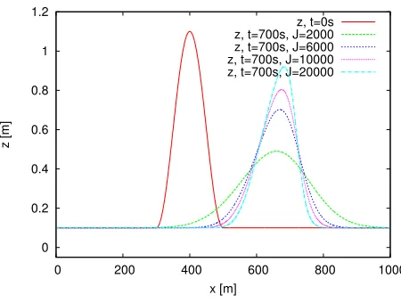
z, t=0s z, t=700s, J=2000 z, t=700s, J=6000 z, t=700s, J=10000 z, t=700s, J=20000
Figure 3. 1D dune evolution.
We first consider a classical test case considered in several works (among others [4, 9, 10, 12, 18, 19, 27, 39, 41, 42]), i.e. the evolution of a dune. It is a sediment transport problem in a channel of lengthL= 1000 m. The initial bottom topography is a bump, we have the following initial data
zb(0, x) =
0.1 + sin2 (x
−300)π
200
if 300≤x≤500 m 0.1 elsewhere
h(0, x) = 10−zb(0, x)
u(0, x) = q0
h(0, x)
with q(t,0) =q0= 10 m2/s the inflow discharge. Thus the flow is sub-critical. Fluid velocity increases as the
dune. For this test, we consider the Exner’s law with the Grass formula (2): Ag = 1 and mg = 3. Thus we have a fast speed of interaction between water flow and bed-load. For the simulation time, we have taken
T = 700 s, as in [9] in order to validate our results. Four uniform grids are considered for the discretization of the computational domain composed byJ = 2000, 6000, 10000 and 20000 cells. We recover kinematics obtained in [9]. WithJ = 2000 cells, we notice that the numerical method is diffusive (Fig. 3). Adding cells improves the results. With these results, the 2D code parallelization is fully justified. The numerical method is suitable for sub-critical flow where dune phenomenon occurs. With the following test, we will see that, it is suitable for supercritical flow as well.
5.2.
1D antidune evolution
With this test we consider a configuration which allows the occurrence of the anti-dune phenomenon. The channel is L= 24 m long. The initial data are a topography with a parabolic bump
zb(0, x) =
0.2−0.05 (x−10)2 if 8≤x≤12 m
0 elsewhere ,
a uniform dischargeq(0, x) =q0= 1.7 m2/s and the water height is the stationary supercritical profile (for the
Shallow Water equations) obtained thanks to Bernoulli’s law
q(t, x) =q0 q2
0
2gh2 +h+zb=H0
where H0 = q
2 0
2gh2
0 +h0+zb(0,0) is the total hydraulic head at inflow (Fig. 4 top left). The water height at inflow is h(t,0) = h0 = 0.5 m. This is the opposite conclusion as for the previous test: the speed decreases
before the top of the bump, there is deposition, and after the summit, the speed rises again and thus causes erosion. We get anti-dune going upstream. For this test, we consider the Exner’s law with the Grass formula (2): Ag = 0.001 and mg = 3. The simulation time is T = 50 s and the computational domain is divided into
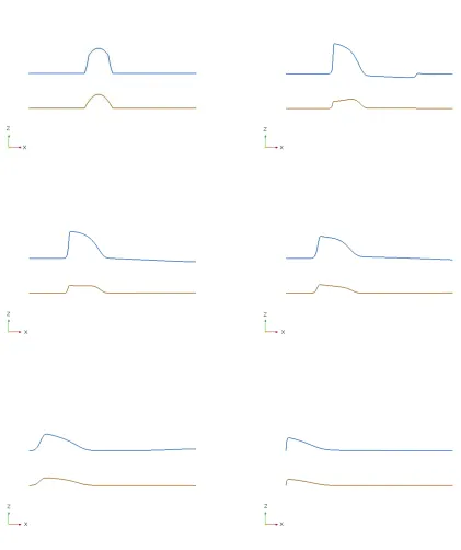
J = 2400 space cells. On Fig. 4, we notice the propagation of the anti-dune upstream (from right to left). This phenomenon has already been studied theoretically et experimently (see e.g. [21, 22, 37, 38, 47, 59]), but up to us, it is the first time that anti-dunes are simulated numerically.
5.3.
2D dune evolution cases
In these classical purely two-dimensional tests, considered in many publications (see e.g. [4, 9, 10, 16, 19, 25, 27, 39, 40]), we study the evolution of a bump in a channel (Fig. 5). The dimensions of the domain are (Lx×Ly) = (1000m×1000m). The initial data common to each test are
zb(0, x, y) =
0.1 + sin
π(x−300)
200
2
sin
π(y−400)
200
2
if (x, y)∈[300,500m]×[400,600m]
0.1 elsewhere
h(0, x, y) = 10−zb(0, x, y)
u(0, x, y) = q0
h(0, x, y)
v(0, x, y) = 0
with u(resp. v) the velocity in x(resp. y) direction andq0 = 10m2/s the upstream constant discharge inx
Figure 4. Antidune evolution for different times 0s, 6s, 10s, 15s, 30s and 50s.
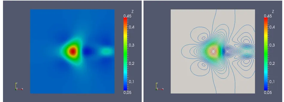
5.3.1. Fast interaction –Ag= 1
Figure 5. 2D bump - initial condition.
Figure 6. 2D bump atT = 500 s forAg= 1.
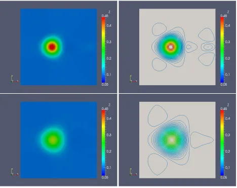
5.3.2. Intermediate interaction –Ag= 0.1
For this test, intial data are those described previously with Ag = 0.1. The simulation time is T = 1000 s and the computational domain is divided into (J×K) = (4000×4000) cells. At the location of the of the bump, we notice that the method is diffusive (Fig. 7): indeed, we have circles on the pictures representing contours. However, as for the previous test, the overall shape is correct.
In order to evaluate the speed-up, we ran the simulation on 4, 8, 16, 32 and 64 cores. The computation time and acceleration are represented on Fig. 8. Usually, speed-up is defined byS =T1/Tp, with pthe number of
processors,T1the execution time of the sequential algorithm andTpthe execution time of the parallel algorithm
with pprocessors. Thus speed-up is a very classical criteria to know how much a parallel algorithm is faster than a corresponding sequential algorithm (see among others [30, 31] and [58]). A linear speed-up or ideal speed-up is obtained when Sp =p. In our case, performing the sequential code was too consuming, thus we have usedT4 as the reference. The ”speed-up” is calculated as what follows: S = 4T4/Tp. We get a speed-up
Figure 7. 2D bump evolution atT = 500 s (up) and T = 1000 s (down) forAg= 0.1.
machines of the last generation, hybrid parallelization should be considered. Using OpenMP with MPI could increase benefits like: memory saving, better load balancing and better adequacy to the hardware specificities.
6.
Conclusions and perspectives
The objective of this work was to prove that the relaxation solver that we introduced in [3] is adapted to reproduce
• well known physical phenomena as the anti-dune process that are not so easy to handle at the numerical level, in particular when soft coupling (i.e. independent solvers or fluid and solid parts) are considered as it is mostly the case for industrial applications,
• two dimensional situations when coupled with a parallelization procedure.
0 4000 8000 12000 16000 20000
0 8 16 24 32 40 48 56 64
T
im
e
(
mi
n
)
Nb cores
ideal MPI
0 8 16 24 32 40 48 56 64
0 8 16 24 32 40 48 56 64
S
p
ee
d
u
p
Nb cores
Figure 8. CPU time and speedup forAg= 0.1.
layer by considering a more complete system for which energy equation can be exhibited. This can be done by considering formal reduction procedure starting from three dimensional model (in the spirit of [34] for classical shallow water system) or by directly introducing adapted multilayer models, see for example [62]. The other one is to improve the fluid model. Indeed, performing linear stability analysis can show that the Saint-Venant equations, which is a averaged models, do not admit instability rising on the bed from a suitable initial pertur-bation contrary to those observed in real life. This relative failure of the models led to the consideration of a full fluid flow model, in which, rather than supposing that the flow is shear free and that viscous effects were confined to a turbulent boundary layer, rotational effects were considered, and a model of turbulent shear flow incorporating an eddy viscosity, together with the Exner equation for bedload transport, was adopted (see e.g. [14, 20, 21, 28, 29, 48, 49]).
Acknowledgments
O. Delestre, R. Serra, H. Le Minh thank CaSciModOT federation (Calcul Scientifique et Mod´elisation Orl´eans Tours) and AMIES agency (Agence pour les Math´ematiques en Interaction avec l’Entreprise et la Soci´et´e) for financial support. E. Audusse and M. Masson-Foucher thank PEPS project (Projets Exploratoires Premier Soutien pour les Interactions Math´ematiques-Informatique-Ing´enierie) initiated by INSMI for financial support.
References
[1] E. Audusse and M.-O. Bristeau. A well-balanced positivity preserving ”second-order” scheme for shallow water flows on unstructured meshes. Journal of Computational Physics, 206:311–333, 2005.
[2] E. Audusse, F. Bouchut, M.-O. Bristeau, R. Klein, and B. Perthame. A fast and stable well-balanced scheme with hydrostatic reconstruction for shallow water flows. SIAM J. Sci. Comput., 25(6):2050–2065, 2004.
[3] E. Audusse, C. Berthon, C. Chalons, O. Delestre, N. Goutal, M. Jodeau, J. Sainte-Marie, J. Giesselmann, and G. Sadaka. Sediment transport modelling : Relaxation schemes for Saint-Venant - Exner and three layer models. ESAIM: Proc., 38:78–98, 2012. URLhttp://dx.doi.org/10.1051/proc/201238005. [4] F. Benkhaldoun, S. Sahmim, and M. Sea¨ıd. A two-dimensional finite volume morphodynamic model on
unstructured triangular grids. International Journal for Numerical Methods in Fluids, 2009.
[5] F. Benkhaldoun, S. Sahmim, and M. Sea¨ıd. Solution of the sediment transport equations using a finite volume method based on sign matrix. SIAM J. Sci. Comp, 31:2866–2889, 2009.
[6] A. Berm´udez and M.E. V´azquez. Upwind methods for hyperbolic conservation laws with source terms.
[7] A. Berm´udez, A. Dervieux, J.-A. Desideri, and M. Elena V´azquez. Upwind schemes for the two-dimensional shallow water equations with variable depth using unstructured meshes. Computer Methods in Applied Mechanics and Engineering, 155(1-2):49–72, 1998. ISSN 0045-7825. URLhttp://www.sciencedirect.
com/science/article/B6V29-3WN739F-4/2/3120ee07ea5c43b3318fbfb6c05d2dde.
[8] C. Berthon, S. Cordier, O. Delestre, and M.-H. Le. An analytical solution of the shallow water system coupled to the Exner equation. Comptes Rendus Mathematique, 350(3–4):183–186, 2012. ISSN 1631-073X.
URLhttp://www.sciencedirect.com/science/article/pii/S1631073X12000088.
[9] M. Bilanceri, F. Beux, I. Elmahi, H. Guillard, and M.V. Salvetti. Linearised implicit time-advancing applied to sediment transport simulations. Technical Report 7492, INRIA, 2010.
[10] D. Bresch, M.J.C. D´ıaz, E.D. Fern´andez-Nieto, A.M. Ferreiro, and A. Mangeney. High order finite volume methods applied to sediment transport and submarine avalanches. In Sylvie Benzoni-Gavage and Denis Serre, editors,Hyperbolic Problems: Theory, Numerics, Applications, pages 247–258. Springer Berlin Hei-delberg, 2008. ISBN 978-3-540-75711-5. URLhttp://dx.doi.org/10.1007/978-3-540-75712-2\_20. [11] I. Brugeas. Utilisation de MPI en d´ecomposition de domaine, March 1996. URLhttp://www.idris.fr/
data/publications/mpi.ps.
[12] V. Caleffi, A. Valiani, and A. Bernini. High-order balanced CWENO scheme for movable bed shallow water equations. Advances in Water Ressources, 30:730–741, 2007.
[13] B. Camenen and M. Larson. A general formula for non-cohesive bed load sediment transport. Estuarine Coastal and Shelf Science, 63:249–260, 2005.
[14] C. Camporeale and L. Ridolfi. Nonnormality and transient behavior of the de Saint-Venant-Exner equations.
Water Resources Research, 45(8):n/a–n/a, 2009. ISSN 1944-7973. URLhttp://dx.doi.org/10.1029/ 2008WR007587.
[15] A. Canestrelli, M. Dumbser, A. Siviglia, and E. Toro. Well-balanced high-order centred schemes for non-conservative hyperbolic systems. applications to shallow water equations with fixed and mobile bed. Ad-vances in Water Ressources, 32:834–844, 2009.
[16] A. Canestrelli, M. Dumbser, A. Siviglia, and E. Toro. Well-balanced high-order centered schemes on unstructured meshes for shallow water equations with fixed and mobile bed.Advances in Water Ressources, 33:291–303, 2010.
[17] M.J. Castro, A. Pardo, and C. Par`es. Well-balanced numerical schemes based on a generalized hydrostatic reconstruction technique. Mathematical Models and Methods in Applied Sciences, 17(12):2065–2113, 2007. [18] M.J. Castro-D´ıaz, E.D. Fern´andez-Nieto, and A.M. Ferreiro. Sediment transport models in shallow wa-ter equations and numerical approach by high order finite volume methods. Computers & Fluids, 37 (3):299–316, March 2008. ISSN 0045-7930. URLhttp://www.sciencedirect.com/science/article/ B6V26-4PSK8R5-1/2/9043410cc90abc43b410c70660a4efd6.
[19] M.J. Castro D´ıaz, E.D. Fern´andez-Nieto, A.M. Ferreiro, and C. Par´es. Two-dimensional sediment transport models in shallow water equations. a second order finite volume approach on unstruc-tured meshes. Computer Methods in Applied Mechanics and Engineering, 198(33-36):2520–2538, 2009. ISSN 0045-7825. URL http://www.sciencedirect.com/science/article/B6V29-4VWB151-1/2/ b1cf68d800ba7d81d182133a1945bc35.
[20] F. Charru and H. Mouilleron-Arnould. Instability of a bed of particles sheared by a viscous flow.
Jour-nal of Fluid Mechanics, 452:303–323, 1 2002. ISSN 1469-7645. URL http://dx.doi.org/10.1017/
S0022112001006747.
[21] M. Colombini. Revisiting the linear theory of sand dune formation. Journal of Fluid Mechanics, 502:1–16, 2004. ISSN 1469-7645.
[22] M. Colombini and A. Stocchino. Finite-amplitude river dunes. Journal of Fluid Mechanics, 611:283–306, 8 2008. ISSN 1469-7645. URLhttp://dx.doi.org/10.1017/S0022112008002814.
[24] G. Dal Maso, P.G. Lefloch, and F. Murat. Definition and weak stability of nonconservative products. J. Math. Pures Appl. (9), 74(6):483–548, 1995. ISSN 0021-7824.
[25] J. De Dieu Zabsonr´e, C. Lucas, and E. Fern´andez-Nieto. An energetically consistent viscous sedimentation model. Mathematical Models and Methods in Applied Sciences, 19(03):477–499, 2009. URL http://www. worldscientific.com/doi/abs/10.1142/S0218202509003504.
[26] O. Delestre, C. Lucas, P.-A. Ksinant, F. Darboux, C. Laguerre, T.-N.-Tuoi Vo, F. James, and S. Cordier. SWASHES: a compilation of Shallow Water Analytic Solutions for Hydraulic and Environmental Studies.
International Journal for Numerical Methods in Fluids, 72(3):269–300, 2013. ISSN 1097-0363. URL
http://dx.doi.org/10.1002/fld.3741.
[27] A.I. Delis and I. Papoglou. Relaxation approximation to bedload sediment transport. Journal of Compu-tation and Applied Mathematics, 213:521–546, 2008.
[28] O. Devauchelle, L. Malverti, E. Lajeunesse, P.-Y. Lagree, C. Josserand, and K.-D. Nguyen Thu-Lam. Stability of bedforms in laminar flows with free surface: from bars to ripples. Journal of Fluid Mechanics, 642:329–348. ISSN 1469-7645. URLhttp://dx.doi.org/10.1017/S0022112009991790.
[29] Olivier Devauchelle, Christophe Josserand, Pierre-Yves Lagr´ee, and St´ephane Zaleski. Morphodynamic modeling of erodible laminar channels. Phys. Rev. E, 76:056318, Nov 2007. URLhttp://link.aps.org/ doi/10.1103/PhysRevE.76.056318.
[30] H. El-Rewini and M. Abd-El-Barr. Advanced Computer Architecture and Parallel Processing (Wiley Series on Parallel and Distributed Computing). Wiley-Interscience, 2005. ISBN 0471467405.
[31] George Em Karniadakis and Rober M. Kirby II.Parallel Scientific Computing in C++ and MPI. Cambridge University Press, 2003.
[32] F.M. Exner. Uber die wechselwirkung zwischen wasser und geschiebe in fl¨¨ ussen. Sitzungsber., Akad. Wissenschaften, pt. IIa:Bd. 134, 1925.
[33] M. Garcia. Sedimentation engineering: Processes, measurements, modeling and practice. ASCE Manuals and Reports on Engineering Practice No. 110, 2008.
[34] J.-F. Gerbeau and B. Perthame. Derivation of viscous Saint-Venant system for laminar shallow water; numerical validation. Discrete Contin. Dyn. Syst. Ser. B, 1(1):89–102, 2001. ISSN 1531-3492.
[35] A.J. Grass. Sediment transport by waves and currents. SERC London Cent. Mar. Technol, Report No. FL29, 1981.
[36] J. M. Greenberg and A.-Y. LeRoux. A well-balanced scheme for the numerical processing of source terms in hyperbolic equation. SIAM Journal on Numerical Analysis, 33:1–16, 1996.
[37] H. P. Guy, D. B. Simons, and E. V. Richardson.Summary of alluvial channel data from flume experiments. Geol. Survay Prof. Paper 462-I, 1966.
[38] L.-H. Huang and Y.-L. Chiang. The formation of dunes, antidunes, and rapidly damping waves in alluvial channels. International Journal for Numerical and Analytical Methods in Geomechanics, 25(7):675–690, 2001. ISSN 1096-9853. URLhttp://dx.doi.org/10.1002/nag.147.
[39] J. Hudson.Numerical techniques for morphodynamic modelling. PhD thesis, University of Reading, October 2001.
[40] J. Hudson and P. K. Sweby. A high-resolution scheme for the equations governing 2d bed-load sediment transport. International Journal for Numerical Methods in Fluids, 47(10-11):1085–1091, 2005. ISSN 1097-0363. URLhttp://dx.doi.org/10.1002/fld.853.
[41] J. Hudson and P.K. Sweby. Formulations for numerically approximating hyperbolic systems governing sediment transport. J. Sci. Comput., 19(1-3):225–252, December 2003. ISSN 0885-7474. URL http: //dx.doi.org/10.1023/A:1025304008907.
[42] J. Hudson, J. Damgaard, N. Dodd, T. Chesher, and A. Cooper. Numerical approaches for 1d morphody-namic modelling. Coastal Engineering, 52:691–707, 2005.
[44] S. Jin and X. Wen. efficient method for computing hyperbolic systems with geometrical source terms having concentrations. J. Comput. Math., 22:230–249, 2004.
[45] S. Jin and X. Wen. Two interface type numerical methods for computing hyperbolic systems with geomet-rical source terms having concentrations. SIAM J. Sci. Comp., 26:2079–2101, 2005.
[46] J.-F. Kennedy. The formation of sediment ripples, dunes, and antidunes.Annual Review of Fluid Mechanics, 1(1):147–168, 1969. URLhttp://www.annualreviews.org/doi/abs/10.1146/annurev.fl.01.010169. 001051.
[47] John F. Kennedy. The mechanics of dunes and antidunes in erodible-bed channels. Journal of Fluid Mechanics, 16, 1963. .
[48] K. K. J. Kouakou and P.-Y. Lagr´ee. Evolution of a model dune in a shear flow. Eur J Mech
B Fluids, 25(3):348–359, October 2005. ISSN 0997-7546. URL http://pubget.com/paper/pgtmp_
4e1e901b36d5a552b68e97d95e82086a.
[49] P.-Y. Lagr´ee. A triple deck model of ripple formation and evolution. Physics of Fluids, 15(8):2355–2368, 2003. URLhttp://link.aip.org/link/?PHF/15/2355/1.
[50] M.-H. Le. Mod´elisation multi-´echelle et simulation num´erique de l’´erosion des sols de la parcelle au bassin versant. PhD thesis, Universit´e d’Orl´eans (in French), available from TEL: http://tel.archives-ouvertes.fr/tel-00780648, November 2012.
[51] R.J. LeVeque. Balancing source terms and flux gradients in high-resolution Godunov methods: The quasi-steady wave-propagation algorithm. Journal of Computational Physics, 146(1):346–365, 1998. ISSN 0021-9991. URL http://www.sciencedirect.com/science/article/B6WHY-45J58TW-22/2/ 72a8af8c9e23f63b0df9484475f7e2df.
[52] Q. Liang. A coupled morphodynamic model for applications involving wetting and drying. J. Hydrody-namics, 23(3):273–281, 2011.
[53] Q. Liang and F. Marche. Numerical resolution of well-balanced shallow water equations with complex source terms. Advances in Water Resources, 32(6):873–884, 2009. ISSN 0309-1708. URLhttp://www. sciencedirect.com/science/article/B6VCF-4VR9FHT-3/2/5218868dcfded7d34380666f23000855. [54] R. Fernandez Luque and R. van Beek. Erosion and transport of bedload sediment. J. Hydraul. Res., 14
(2):127–144, 1976.
[55] E. Meyer-Peter and R. M¨uller. Formulas for bed-load transport. In 2nd meeting IAHSR, Stockholm, Sweden, pages 1–26, 1948.
[56] J. Murillo and P. Garc´ıa-Navarro. An Exner-based coupled model for two-dimensional transient flow over erodible bed. Journal of Computational Physics, 229:8704–8732, 2010.
[57] P. Nielsen.Coastal Bottom Boundary Layers and Sediment Transport. World Scientific Pub Co Inc, August 1992. ISBN 9810204736.
[58] P. Pacheco. An Introduction to Parallel Programming. Morgan Kaufmann Publishers Inc., San Francisco, CA, USA, 1st edition, 2011. ISBN 9780123742605.
[59] G. Parker. Sediment inertia as cause of river antidunes. J. Hydraul. Div. ASCE, 101:211–221, 1975. [60] A. Shields. Application of similarity principles and turbulence research to bedload movement.Mitteilunger
der Preussischen Versuchsanstalt f¨ur Wasserbau und Schiffbau, 26:5–24, 1936.
[61] S. Soares-Fraz˜ao and Y. Zech. HLLC scheme with novel wave-speed estimators appropriate for two-dimensional shallow-water flow on erodible bed. Int. J. Num. Meth. Fluids, 66(8):1019–1036, 2010. [62] Y. Zech, S. Soares-Frazao, B. Spinewine, and N. Le Grelle. Dam-break induced sediment movement:
![Figure 1. Plot of several bedload functions found in the literature [33], τ ∗cr = 0.05.](https://thumb-us.123doks.com/thumbv2/123dok_us/10071641.1993580/3.612.117.448.260.405/figure-plot-bedload-functions-literature-t-cr.webp)