http://www.sciencepublishinggroup.com/j/mcs doi: 10.11648/j.mcs.20180304.11
ISSN: 2575-6036 (Print); ISSN: 2575-6028 (Online)
Statistical Considerations on Software-Safety Estimation in
Licensing
Wolfgang Ehrenberger
Department of Applied Informatics, University of Applied Science, Fulda, Germany
Email address:
To cite this article:
Wolfgang Ehrenberger. Statistical Considerations on Software-Safety Estimation in Licensing. Mathematics and Computer Science. Vol. 3, No. 4, 2018, pp. 77-86. doi: 10.11648/j.mcs.20180304.11
Received: May 15, 2018; Accepted: June 22, 2018; Published: July 25, 2018
Abstract:
During the discussions in preparation of the new versions of the International Electrotechnical Commission (IEC) standards IEC 61508-3 and IEC 61508-7, controversies regarding the proper roles of statistical validation or verification of safety-related software have emerged. These controversies regard changing demand profiles and continuous operation versus on-demand operation. This contribution derives a formula for calculating the failure probability per demand of software that has been tested under a demand profile that is different from the profile of its intended use. It also explains how failure rates can be expressed in terms of failure probabilities per demand, if the operational conditions are known. It further describes how software that is alternately operated continuously and on demand can be characterized in statistical terms and how the two operation modes can be recognized during a statistical evaluation. The notion of “mission” is suggested for sequences of demands or mixtures of demand-driven and continuous operation of software. In order to allow statistical calculations many requirements have to be met strictly. They are listed in the appendix. This article can hopefully facilitate licensing of software in many cases. Remarks are invited.Keywords:
Software Safety, Statistical Testing, Operational Experience, One-Sided Confidence Interval, Changing Demand Profile, On-Demand or Continuously Working, Missions1. Introduction
Currently a team of the International Electrotechnical Commission (IEC) is updating its standard about software in safety-related systems. The existing version of IEC 61508-3 allows statistical arguments during licensing of safety-related software [1, 2, 3]. IEC 61508-7-D describes what has to be observed during the licensing process for a certain Safety Integrity Level (SIL) as defined in its part 1 [1]. The existing standard was developed during the 1980ies, for the then prevailing small computers, simple safety-related computer systems and simple tasks to be solved. Now boththe tasks of safety-related computers have become significantly more complex and the capacity of the computers has increased dramatically. Moreover the challenge has come up to use operational experience of software from conventional applications as an argument during the licensing procedure of safety systems. In order to harmonize this with the existing rules, a Technical Specification (TS) has been drafted: IEC 61508-3-1 [2]. In using this, it is desirable, to express the
value of operational experience quantitatively to substantiate the Safety Integrity Level (SIL) classification of the software under consideration. This leads to the problem of different demand profiles of the old and new application and the challenge of combining demand-based views and time-based views.
Illustrating Example problems (Exp_i)
Exp_1: Software, whose demand numbers increase: Software has been used in a factory for a long time every day when work started and switched off after the working shift in the evening; now it is planned to be used over one week continuously. What reliability data are to be expected?
Exp_3: Fukushima: After the loss of the main heat sink of a nuclear power plant, the reactor has to be switched off, the emergency coolant pumps have to be started, the emergency cooling valves have to be opened after a while and then the after-decay heat has to be removed during hours and days. What is the probability of radio-active poisoning of the environment?
Exp_4: Autonomous car driving on a motor way: The computer takes over control from the driver upon entering the motor way. The drive has to be controlled according to the lanes known from the navigation system, the car has to be steered to the desired exit and control has to be given back to the driver. What is the probability of no accident during a given time?
An important problem arises, if software is modified between two applications. As more and more operational experience of software becomes available, e.g. from software in cars, profiting from the old operational experience can make licensing of software cheaper. The insight gained from statistical testing can be considered similar to the insight from operational experience – to a certain degree. In particular one wants to know, which statistical tests have to be performed to complement any existing operational experience. And last but not least we are interested to learn, how reliability arguments change, when our view switches from continuous operation to demand-based operation or vice versa; i.e. how reliability arguments get a different form; and what we have to conclude, if we have a mixture of both types of operation. All this requires adapting the existing formulations of the mentioned standard(s) to the new circumstances. In trying to do so, controversies have come up between the specialists who were included in the discussions.
2. Existing Views
It is not generally agreed yet, how changes of an operational profile of a particular piece of software influences its safety-capability. Closely connected to that is, how software that has successfully fulfilled a certain number of demands can be classified into the existing SIL system, as this is essentially time-based, because it has to meet the thinking of hardware reliability. The existing literature, has not given clear guidance on either of these cases. [4, 5, 6, 7, 8, 9, 10, 11, 12].
Some publications emphasize the currently emerging new problems, e.g. in autonomous driving and express the need of related new testing concepts. [20, 21, 22]. Only few address stratified sampling [11, 12]; but they do it without discussing one-sided confidence intervals. The same applies for a contribution on subdomain testing [25]. Also a recent publication about awareness of the distribution of events in the program’s input space does not refer to one-sided test confidence [26]. And it is one-sided confidence intervals that characterize our case, as we have operational experience or experiments or test cases without observed failures. If any failure had come up, license would not be granted. It is surprising that these questions are still open, since scientific
interest in the validity of statistical observation has existed since a long time. [5, 6, 7].
In addition to the mentioned aspects we have to recognize: Many of those, who drafted the existing standard were very familiar with statistics, because they came from physics. Now colleagues, who have been educated mainly in computer science enter the computer-safety area, and some of them have little expertise in the mathematics of probabilities. This has led to considerable confusion recently, including mis-interpretation of the standard [3]. The following text tries to start from the basic aspects. A pre-publication about the area has been made in German. [19].
3. Software Working on Demand
The software of safety-related digital computers can in most cases be understood as having paths that are started by a specific event, e.g. by an interrupt. The input data are read, the related results are evaluated and put out. The text below is based on definitions that are not used in the same way by all authors. Those that might be controversial are given here:
Path: Traversal or possible traversal of a piece of software from its start to its end; or: program run from its starting timer interrupt to its end; or: sequence of machine instructions that is executed or can be executed;
Demand: Input condition or input conditions from the Equipment under Control (EUC) that lead to the execution of one or several paths with possible safety-related effects;
Demand profile: Set of all input conditions from the EUC that lead to the execution of one or several paths with possible safety-related effects and their number or frequency;
Failure: Output of the execution of a path or demand or of a set of paths or demands that contradicts the specification of the software; effect of a software fault; the random event in this article.
3.1. The Simple Case: Constant Demand Profile
We are looking for the number of test cases or cases of operational experience that are needed to demonstrate:
The failure probability per demand of our software is below a certain limit. That limit shall be valid at a given level of confidence. In other words: The probability Pr that the failure probability per demand p’ is below an upper limit p shall equal β i.e. be true at the level of confidence β.
Formally:
Pr (p’ ≤ p) = β
Here the random variable is p, as the upper limit is to be evaluated. The failure probability p’ is fixed, but unknown. The random event is software failure F. [24].
The formula we are after and its derivation have been widely known. [6]. The derivation is repeated here, because a further conclusion is drawn from an intermediate result.
p: upper limit of the probability of failure per demand; 1-p: lower limit of the probability of no failure per demand. n: number of test cases or demands.
proof by falsification of the complement. Ideal circumstances are assumed, as the requirements from the appendix below prescribe. They are reported here shortly in slightly different wording. We have:
(1) statistically independent test cases,
(2) no failures during test or pre-use operation, (3) no failure masking,
(4) no internal states, or internal states are considered like input variables;
(5) probability of one demand over a small interval is approximately proportional to the size of that interval;
(6) if the software memorizes certain internal values over a certain time, a single test case, run or operational traversal is taken over that time;
(7) the software works purely deterministically.
For a collection of all requirements and their more precise formulations see appendix.
Then it holds:
(1-p)n: probability of no failure at a test with n demands, the complement to having at least 1 failure on n demands. As we argue by falsification of the complement, it has to be small, if a large level of confidence is to be demonstrated: If the original hypothesis were wrong, we must have at least 1 failure.
α: level of significance of a statistical hypothesis; α = 1 – β.
(1-p)n = α (1) level of significance of a test with n demands without failure; to be small. See also [6] and theory of statistical sampling [9]. Taking the logarithm yields n*ln (1-p) = lnα. This leads to n and, because p is small:
n =
p
p
≈
−
−
α
α
ln
)
1
ln(
ln
;n
p
≈
−
ln
α
(2)/*formula from IEC 61508-7 D [3]*/
For the upper limit of the (fictive) number of failures to be expected E(F) from n demands to the given level of significance we get further:
E (F) = n*p. (3)
This is intuitively clear but can also be derived from the Poisson distribution or the binomial distribution. It also follows: E (F) = - lnα.
Should (2) be used for any prediction of future use of the software, it must also hold:
1)Pre-existing or tested code and code of the future application are identical.
2)The demand profile of the test or pre-operational experience is identical to the demand profile of the future application.
In many cases this requirement does not hold, as the way the software is used differs more or less significantly from that of its testing or pre-operation phase. We now examine,
which effects different demand profiles have.
3.2. Several Types of Executions, Changing Demand Profile
The considerations of this article refer to conventional digital computers. Their software is understood as being executed sequentially, machine command per machine command. A sequence of machine commands from program start to its end is called a path. Our software is assumed to have K different such paths. The ideal pre-requisites except the last-mentioned requirement still apply for each of these; path i is executed ni times.
With n = nt = 1 K i i n =
∑
total number of runs or executions
and p = ptotal = pt, we derive from (1):
1 2
1 (1 )t (1 ) (1 ) ...(1 ) ...(1i )K (1 )i
n K
n n n n n
t t t t t i t
p p p p p p
α= − = − − − − =
∏
= −From (3) we can derive: E (F) = nt*pt, as a (fictive) upper limit of the number of failures to be expected from nt demands. If the same level of significance applies for each path:
-lnα = E (Fi ) = E (F) = ni*pi is the upper limit of the number of failures to be expected from the ni demands of path i to the given level of significance. We set:
pt := πi * pi (4)
with
( ) *
( )
t i i
i
i t t
p E F n n
p n E F n
π
= = = (5)to be valid for all paths i. πi is the probability of selecting
path i. This leads to:
(1
)
t 1(1
*
)
in K
n
t i i i
p
p
α
= −
=
∏
=−
π
Since all πi* pi are small, it holds from (2):lnα = nt*ln (1 - pt)
≈
nt (- pt)1 1
ln(1 ) ( )
K K
i i i i i i
i i
n
π
p nπ
p= = ≈
∑
− ≈∑
− and pt 2 1 * K i i i pπ
=≈
∑
(6)This has always some claim for being true, if the requirements mentioned - and perhaps R13 from the appendix are met. It can easily be validated by an example. See Example 2. The set of the πi represents the demand profile of the software. Therefore (6) can be used to evaluate the change of the software failure probability, if the demand profile changes.
If the demand profile changes the relations (4) and (5) do not hold. As the failure properties of the individual paths did
paths, but since πi_new ≠ πi_old and consequently pt_new ≠ pt_old, (4) can no longer be valid for the new demand profile. This was a point during the discussions [24]. The old profile was the “ideal” profile, since the test or operational experience was designed or interpreted according to (4). Therefore we get in all cases pt_new > pt_old for the new demand profile, as illustrated by the following example.
Example 1: Originally we had 2 different paths, numbered i and k, with identical properties: πi_old = πk_old = πold and pi_old = pk_old = pold. So the influence of our pair of paths on
the total failure probability per demand is: πi_old2 *pi_old + πk_old2 *pi_old = 2 πi_old2 *pi_old. For the new
application we assume that πi_new is larger than πi_old. We write πi_new = πi_old + ∆. As the sum of all πi is always 1, we get on the other hand a smaller selection probability of the same size; we assume path k is affected. πk_new = πk_old – ∆. Formula (6) consists of summands that always contain π2. The relation transfers this into πi_new2 *pold + πk_new2 *pold
which is (πi_old + ∆
)
2 *pold + (πk_old - ∆)
2 *pold = pold*(πi_old2 +2 πi_old* ∆ + ∆2 + πi_old2 -2 πi_old * ∆ + ∆2 ) =pold*(2πi_old2 + 2∆2) > 2πi_old2 pi_old from above.
Because of the quadratic relation in formula (6) any deviation of the demand profile from the ideal one leads to an increase of the failure probability per demand of the whole software system. During a practical licensing procedure one can estimate the effect of a profile change by (6) and decide whether or not pt_new still meets the reliability requirements. (6) also suggests that the effect of small changes is not significant, since they influence the result only by squares of numbers smaller than 1.
From (4) we calculate the value of pi_new that would be sufficient to reach pt_new.
_ _
_
t new i new
i new
p
p
π
=
The derivation of (6) is valid only, if a minimal number of runs of each path have been executed, such that (2) is valid for each path. This can be assumed,
1)if the pre-requisites of the Poisson distribution are met. And, of course,
2)if the number of runs of each path is well known both for the old and the new demand profile.
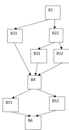
Example 2: A program part consists of 9 basic blocks as depicted in Figure 1. They form 6 paths that are traversed during testing according to the Tables 1and 2. Any Block Bi
is traversed purely sequentially.
Figure 1. Flow graph of a program part with 9 Basic Blocks and 6 paths.
Table 1. Path traversals of the flow graph of a program part according to Figure 1; 9 Basic Blocks, 6 paths, nt = 30000 traversals or runs in total.
Traversals per Basic Block
Block Block traversals nij Paths
1 30000 All
21 20000 1, 2
22 10000 3, 4, 5, 6
31 2500 3, 4
32 7500 5, 6
4 30000 All
51 8000 1, 3, 5
52 22000 2, 4, 6
6 30000 All
Table 2. Path traversals of the flow graph of a program part according to Figure 1; 9 Basic Blocks, 6 paths, nt = 30000 traversals or runs in total.
Traversals per path
Paths Path traversals ni Blocks
1 7000 1, 21, 4, 51, 6
2 13000 1, 21, 4, 52, 6,
3 500 1, 22, 31, 4, 51, 6
4 2000 1, 22, 31, 4, 52, 6
5 500 1, 22, 32, 4, 51, 6
6 7000 1, 22, 32, 4, 52, 6
If α = 0.05, ln 0.05
≈
-3; from (2): pt = lnt
n
α −
≈
10-4
Table 3. Probabilities of path traversals or runs and upper limits of failure probabilities; numbers from Table 2, calculations of rows 2 according to (4), row 3 according to (2), for -ln α = 3, corresponding to level of confidence of 95%. Row 4 according to (6).
Path number i 1 2 3 4 5 6 all, ∑
Path probability πi 0.23333 0.43333 0.01667 0.06667 0.01667 0.2333 1
Failure probability pi 4.28*10-4 2.31*10-4 60*10-4 15*10-4 60*10-4 4.28*10-4
πi2*pi 2.333*10-5 4.43*10-5 1.666*10-6 6.67*10-6 1.666*10-6 2.333*10-5 10-4
Table 4.Probabilities of path traversals changed, failure probabilities per demand of the paths as above; level of significance also unchanged.
Path number i 1 2 3 4 5 6 all, ∑
Path probability πi_new 0.2 0.01 0.6 0.05 0.05 0.09 1
Failure probability pi 4.28*10-4 2.31*10-4 60*10-4 15*10-4 60*10-4 4.28*10-4
πi_new2*pi 1.71*10-5 2.31*10-8 21.6*10-4 3.75*10-6 1.5*10-5 3.47*10-6 2.2*10-3
Table 4 shows: The failure probability per demand of the changed profile is higher than the original one.
The basic blocks B1 to B 6 of the Figure 1 together can be understood as one module of a program. In both of the considered cases (Tables 2 and 3) the number of demands was identical, only the internal distribution was different. And this led to a different total failure probability. We see from that example: It is extremely difficult, if not impossible to derive failure probabilities per demand from modules only. It is much more accurate to derive these probabilities from the traversed paths.
Memorizing paths and the execution numbers of the paths has already been treated [18]. Gathering path data can be expensive, in some cases impossible. Then one may perhaps conservatively estimate the old and the new ni. A conservative estimate would correspond to the habit of other engineering disciplines to super-dimensioning the related parts of the construction. Demand profiles can also be estimated on the basis of the data that have been or are to be processed in different operation modes. But: If a path that has not been executed during test or pre-operation, it has to be considered as failing, i.e. pi_new= 1, in the new application
and contributing to the total failure probability pt_new with
_ i new
π and not with πi_new2.
3.3. Notes
During the discussion of this section it was put forward
that pt’ = i 1
* ' K
i i
p
π
=
∑
as it applies “normally” in stratifiedsampling [24]. See also related formulae in other publications [11, 12]. They do, however, not consider one-sided confidence intervals that characterize our problem. If e.g. all
pi’ were equal and since 1 K
i i
π
=
∑
= 1, we would get: pt’ = pi’,which contradicts (2) with respect to pt, as it does not recognize that nt > ni applies for all paths i.
Counterexample 1: A colleague reports that licensing on the basis of (6) is not suitable for the products of his company. Many failures including stack overflows were observed after a change of the demand profile.
Explanation: It was never checked whether the old demand profile contained all paths of the new profile.
Counterexample 2: A colleague reports that licensing on the basis of operational experience was not suitable for a product used by his employer: The software had worked well for a long time for a limited operational period during each day. It failed due to overflow of a counter, as it was used continuously for a longer period than a day.
Explanation: The individual executions of the software were not statistically independent. They were coupled via a
counter and the user was not aware of this.
Licensing on the basis of the formulae given in this contribution is only feasible if the mentioned pre-requisites are met. See appendix. Demonstrating this may be time consuming and costly. In some applications it is cheaper to do verification in a systematic way.
4. Continuous Operation and Demand
Operation
In many cases several views on one and the same item are possible: e.g. light can be considered as particles or waves; or solving a particular task can be considered as a sequence of single subtasks or as a continuous effort. So is it with the work of digital computers. They can be considered as being driven by sequences of events from the EUC or by continuous input data from the EUC. All digital computers work, however, more or less demand-driven; in contrast to analog computers.
4.1. Operation on Demand
In industrial applications a digital computer operates frequently on demand, say by polling, each reading cycle is started by an interrupt; interrupts coming at constant time intervals from outside. The safety-related functions of the computer may act in case of danger to the EUC that is supervised. A demand consists of a combination of input parameters from the EUC that can cause danger; a software failure would be an improper reaction to the demand. Another view of this functionality may consider the input data gained by polling as used for continuous control, in keeping the output variables in pre-defined limits: After each reading of the inputs the new outputs are evaluated and sent.
4.2. Software Working Continuously
confidence or significance, say
Pr (λ’ ≤ λ) = β = 1 – α.
Consequently, the upper limit of the number of failures E (F) that is expected to a certain level of confidence during operation time t can be estimated as
E(F) = t*λ. (7)
In the on-demand view we have the upper limit of the number of failures according to (3). As the number of failures cannot depend on the view on a system, it always holds for n demands during operation time t:
n*p = t*λ, (8)
if the pre-requisites mentioned in the appendix apply. As t and n have fixed values, λ is the upper limit of the real λ’ at the same level of confidence as p is the upper limit to p’. Under ideal circumstances one can use (8) for calculating λ from n and p, if t is known, or deriving p from λ, n and t.
This consideration is plausible because we are dealing here with digital computers and a digital computer is always working on demand. It is, however, in some cases more convenient to consider it as a continuously working device. From (8), (3) and (7) it follows
ln
t
α
λ
= − , (9)
which is obviously similar to (2) and gives the necessary testing time or time of operational experience to support a certain failure rate at a certain level of significance.
If the claimed pre-requisites do not hold, the left hand side of (8) cannot be evaluated and therefore the formula is not applicable. Never the less its right-hand side may get a value by applying the exponential distribution on the observed data. More detailed considerations on the problem and its terminology exist [14].
(8) can also be used to evaluate the effect of squeezing the (fictive) operation time during testing if a certain value for λ
is to be demonstrated.
Example 3: A program has been executed under ideal conditions with 30000 demands, each demand corresponding to two operational hours, t = 2*30000 h. We get: from (3) n*p = 3 = -lnα. (9) leads to:
* 3
2 * 30000 n p
t
λ
= = and λ’ ≤ 0.5*10-4 1/h at a level ofsignificance of 0.05.
Should the program be used with a higher demand rate, say 1 per hour, and should the same λ at the given confidence level be required, one would need 60000 demands to demonstrate that λ is still below the derived limit at the mentioned level of significance. These 60000 demands need not take 120000h. If all details are known, testing time can perhaps be reduced to 120 hours, or even less by increasing the demands per time unit.
If the real operational environment requires proper
reaction for each demand in more than 2 hours only, further calculations on the level of the whole safety-related system will just need a smaller λ.
Calculating failure rates from failure probabilities per demand is important, since IEC 61508-1 defines SILs essentially on the basis of failure rates [1]. In that standard failure probabilities per demand are listed only for demands that occur less than once per year. Many licensing processes demonstrate the capabilities of the involved EUC hardware by fault trees or Markov chains that use failure rates. So deriving failure rates for digital computer software can be helpful during licensing.
Using (6) and (8) one can estimate the failure rates for applications, where several types of continuous demands apply and change. One should, however, remind that (8) is not easily applicable to analog computers. Some more detailed considerations of the here discussed problems have been published from other points of view, without considering confidence limits, however [14, 27].
4.3. Software with Memory
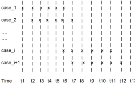
Until now we have clandestinely assumed that the software system examined is memory-less. If our software has to control some EUC continuously it may be required to keep some memory of what has happened before, as analog controllers used to do. It is assumed that the software works by polling, with constant intervals of ∆t, e.g. being started by an external interrupt after each interval. So its control flow of each case or path is:
1 Read sensor signals from EUC
2 Calculate results, considering earlier intermediary results as far as needed
3 Issue control commands to EUC
In this case the timing of Figure 2 applies. A test case runs over 5 time steps. The individual cases overlap and can be evaluated independently, if they do not interact. If they do, the time period of the influence of one such interaction has to be taken into account. Then one test case runs over the whole period of the possible influence of an input. It might then be better to apply the notion of missions as the section 5 suggests.
4.4. Mixed Processes
In some applications one result can be affected by different types of causes: continuous ones and demand-driven ones. This is normally visible from the requirements specification of the software. It is then difficult or impossible to apply the formulae of this contribution directly. It may be necessary to investigate the software code in detail.
5. Missions
In some cases neither the demand-oriented nor the continuous view is the most appropriate one. Demands and continua can appear in a mixed way. It is then reasonable to take some super view: the mission.
Example 4: The Anti-Blocking System (ABS) of the wheels of a car is triggered by blocking of one or several of its wheels, if the driver brakes. If the ground is slippery, the ABS may be needed for a certain time till the car stops. It is reasonable to consider the whole sequences of actions on all wheels of the car as one demand, better, as one mission. Reliability considerations take care of the different types of the individual missions that the breaking system has to master and their frequency.
Example 5: Some cars switch off their motors, if the car stops and start it again, if the driver wants to go on. The sequence of actions that the investigated software system has to take between a start and the next stop can be treated as a unity, as one mission. Such missions can last for seconds or for hours.
The earlier considerations of this article suggest to treating one mission as one super demand, consisting of several types of “normal” demands mixed with several types of continua and gather information on the different types of such super demands. Should the (super-) demand profile change, e.g. a car being used more frequently in another environment, (6) can form a basis for estimating the safety or reliability properties in that environment; e.g. different uses of the ABS by people who use to go skiing or normal drivers. Of course the paths that are traversed during the two types of operations have to be identified and the number of their traversals need to be known or conservatively estimated.
6. Conclusion
Statistical considerations can help in evaluating the safety properties of software. In some circumstances they are the preferred means for getting quantitative results. Their use may, however, cause much effort in gathering data and do the modelling that is required to get meaningful results. In practical cases engineers will not only rely on the formulae given here, but do what engineers always do, if reliability is an issue: Consider a safety margin.
It is normally also quite time consuming to verify that the pre-requisites are met that are needed to allow a statistical approach. The efforts for statistical assessment may be larger than the efforts needed to do program analysis,
analysis-based testing and related proving. Statistics can mainly be helpful as a complementary venture to the deterministic way of software validation and verification; in particular, if large and well-documented operation experience exists. It can never be the only way of verifying the correct or safe behaviour of software.
In order to keep this article focused on the essential aspects, some points that might be important to the reader have been left out; like: How do inaccuracies of the knowledge of the demand profile influence the desired result? Or: What is a reasonable precise definition of a path, or: How can path traversals or runs be characterised and stored and how can the stored information be retrieved easily? See [18].
The illustrating example problems from the Introduction can be solved as follows:
Exp_1 Use (8) and compare with the required safety margins. Exp_2 Use (6) and (8)
Exp_3 Use (8) for calculating the resulting failure probability (n=1) for after-decay heat removal; multiply the complements of the failure probabilities per demand.
Exp_4 Use the applicable mixture of demand driven events and continuous periods.
Deriving a whole safety case on the basis of statistical data always causes a lot of calculation effort, similar to the effort for preparing licensing documents for any type of hardware. In particular demonstrating that all needed pre-requisites are met can need deep understanding of the software at stake. In some cases, however, applying statistics can safe work.
Acknowledgements
I thank my colleagues Oleg Taraszow, Anatol Badach and Tim Grams for their critical review of the mathematics of this text and many others for not agreeing with my views; they have helped clarifying the thoughts of this article. I also thank the reviewer of the publisher. Ian Pyle, Ron Pierce and cooperators of the publisher have checked the correctness of the English expressions; thank you!
Appendix
Collection of Pre-requisites and Assumptions
A.1 General Pre-requisites for Licensing on Proven in Use Arguments from [2, 3]
The conditions of use (operational profile) of software include all the factors that may trigger systematic faults. To find out, whether one can use operating experience in a safety case, one has to compare the old and the new operating profile. To determine whether two operational profiles are identical or sufficiently similar documentary evidence shall demonstrate that the following features and phenomena of previous use are identical in the intended use of the element in the E/E/PE safety-related system:
a)Software environment (e.g. processor, memory, clock, bus behavior, demand profile);
program variables and constants, the hardware configuration on which the software will execute); c)software interfaces;
d)libraries (including source code libraries as well as libraries of binary code);
e)operating systems, interpreters (for example, those used to emulate processor architectures on processors which do not share that architecture);
f) translator (compiler), linker, code generators;
g)contain a complete description of the conditions of use of the proven-in-use software.
A.2 Detailed Aspects About Software Functions (in Part from [2, 3]).
The following rules, requirements and assumptions apply for software functions of all safety-integrity levels (SILs). They concern properties of the software, of operational experience and statistical test cases. Operational experience can supplement or replace statistical testing, and operational experience from several sites may be combined (i.e. by adding the number of treated demands or hours of operation). The following text refers always to the code (software) of functions and NOT to (software) modules or code parts.
Trivial aspects
R1 The codes of the pre-existing or tested functions for which operating experience is claimed and the code of the functions for the future intended application are identical.
Note 1: This can be demonstrated by proper use of hash functions.
Note 2: Identity of software version means fundamentally the identity of binaries. This can occasionally lead to problems where a binary code runs in emulation mode. Then hardware and emulator are to be taken into account.
R2 No failures have occurred during pre-operation or test. This includes:
R2a The software has always worked correctly.
R2b Observation of information gathering has been so strict and complete that any possible incorrect behavior has been recognized.
R2c A specification has existed (and still exists) that has allowed to decide whether any result was correct of incorrect. Note: If this is not fulfilled, the software will not be licensed for any safety-related application.
To be met by the software to be evaluated
R3 The software is a pure function of its input data; one treatment of a subset of the actual set of input data that causes an output is called one run or one traversal; each run is represented by one path; sequence and number of runs of any path cannot influence any future run; or see also R5, R6 and R7.
R4 No failure masking has occurred during testing or pre-operation [15].
Note1: For example the software may be required to react on two external events. It may have reacted correctly under all tested circumstances, but event 1 was always faster than event 2. So no experience exists on any possible failure to react on event 2.
Note 2: Failure masking is always possible if one result is
calculated via an OR-decision.
R5 If the software has internal states, they have to be considered like states of input variables.
R6 The probability of observing one demand over a small interval is approximately proportional to the size of that interval.
R7 If the software memorizes certain internal values over a certain time, a single test case, run or operational traversal shall be taken over that time.
Note1: This view can be helpful, if a control algorithm uses data from the immediate past, e.g. by integration.
Note2: In some cases it may be reasonable not to consider runs of the software but missions as a basis for safety calculations.
R8 No software failure must be able to cause or hide any other software failure (be free from interference).
R9 The software must be executed purely
deterministically.
Note: This is normally the case with a digital computer; the software has no random number generator.
To be met by the test harness or the operational environment that provides the experience
R10 During the operational experience or the tests the individual runs have to be statistically independent from each other.
Note: This means: No single run can influence the result of any other run; or: The test harness or the application where the operational experience has been gathered is or was memory-less from path to path.
R11 Test cases or operationalexperience cases have been selected according to the intended operational profile.
Note: This is not needed, if formula (6) can be applied for correcting any mismatch.
R12 The distribution of input data that are processed in one execution path of the software is similar between the experience gathering during pre-operation or the testing period and the future operation period (equal demand profile within one path).
R13 The number of test cases in each path meet the requirements to be fulfilled for the Poisson distribution. If this is not the case, the related path shall be treated with pi = 1.
R14 The paths and their number of executions are known
from both the previous and the future demand profile.
A.3 Guidelines for Work and Evaluation of Results
G1 The paths shall be identified for the old and the future demand profile.
Note 1: If the new demand profile is just a subset of the old one, no problems exist.
Note 2: If the new profile is not a subset of the old one and if re-calculation is not wanted, any possible short comings can be compensated by additional tests of the paths that were not tested sufficiently yet.
Note 3: Small discrepancies between the profiles can perhaps be shown to be irrelevant by using the well-established rules for dealing with inaccurate measurements.
model checking can help.
G3 the failure probabilities per demand and the number of runs shall be evaluated or conservatively estimated for each path.
G4 Each path that has not been traversed at all shall be considered with failure probability 1 and the probability of its traversal shall be considered without the square (
π
i andnot 2 i
π ).
G5 Concatenated subsequent paths over modules can be considered in software system safety evaluation as one path, if they do not interact; in his case the largest failure probability per demand of any path of the chain shall be taken.
G6 If interacting modules are concatenated, the paths from start to end of the whole software shall be taken.
G7 Paths whose correctness has been proven, shall be considered with failure probability 0.
G8 It is recommendable to verify the correctness of loops
with varying repetition numbers deterministically, e.g. by proof.
G9 Separate considerations are required for complicated
logical expressions or for complicated algorithms.
Note: A logical expression can usually be decomposed into a sequence of branches, and a sequence of branches can sometimes be transferred into a logical expression for one branching instruction.
G10 Some aspects, e.g. actions that shall be triggered by the software at a specific future calendar date, need deterministic verification and white box testing.
G11 When the software safety requirements can formally and rigorously be separated from the overall software requirements then the conditions from above may be applied to safety-related failures of the software only.
G12 Due to the pre-requisites given, a pure random evaluation of low failure probabilities or failure rates is impossible; at least reading of the code and a minimum of understanding is required for software that works on the EUC immediately.
References
[1] ISO/IEC 61508-1: Functional Safety of electrical/electronic/ programmable electronic safety-related systems, Part 1: General requirements (2010) Beuth Verlag Berlin or IEC Geneva.
[2] IEC/TS 61508-3-1 Ed. 1.0: Functional safety of electrical/ electronic/programmable electronic safety-related systems - Part 3-1: Software requirements - Reuse of pre-existing software elements to implement all or part of a safety function, (2015), IEC Geneva or Beuth Verlag Berlin.
[3] ISO/IEC 61508-7: Functional Safety of electrical/electronic/ programmable electronic safety-related systems, Part 7 Annex D (2010), IEC Geneva or Beuth Verlag Berlin.
[4] Baldoni, Roberto; Giorgia Lodi, Luca Montanari, Guido Mariotta, and Marco Rizzuto: Online Black-Box Failure Prediction for Mission Critical Distributed Systems, 31. International Conference Safecomp 2012, LNCS 7612, pp 111-123.
[5] Strigini, Lorenzo and Bev Littlewood, Guidelines for Statistical Testing (Report No. PASCON/WO6-CCN2/TN12). ESA/ESTEC project PASCON) London City University (1997) to be received via the authors.
[6] Butler, Ricky W. and George B. Finelli: The Infeasibility of Quantifying the Reliability of Life-Critical Real-Time Software; IEEE Transactions on Software Engineering, Vol 19, No1 (1993).
[7] Littlewood, Bev and Lorenzo Strigini: Validation of Ultra-high Dependability for Software-based Systems, Communications of the ACM, 36(11), (1993).
[8] Kuball, Silke; John May and Gordon Hughes: Structural Software Reliability Estimation; Safecomp 99, Lecture Notes in Computer Science, Vol. 1698, Springer pp 336-349. [9] Glaß, Michael; Heng Yu, Felix Reimann and Jürgen Teich:
Cross-Level Compositional Reliability Analysis for Embedded Systems 31 International Conference Safecomp 2012, LNCS 7612, Springer pp 111-123.
[10] Cotroneo, Domenico; Domenico Di Leo, Roerto Natella and Roerto Pietrantuono: A Case Study on State-Based Robustness Testing of an Operating System for the Avionic Domain, 30th International Conference, Safecomp 2011, LNCS 6894, Springer, pp 213-227.
[11] Saifuddin, Ahmed: Methods in Survey Sampling Biostat 140. 640 – Stratified Sampling. pdf, (lecture notes) John Hopkins University, Bloomberg, school of public health (2009). [12] de Vries, Pieter G.: Sampling Theory for Forest Inventory –
Stratified Sampling, ISBN 978-3-642-7 1581-5 (1986) Springer. [13] Gran, Björn Axel; Gustav Dahll, Siegfried Eisinger, Eivind. J.
Lund, Jan Gerhard Norstrom, Peter Strocka and Britt J. Ystanes: Estimating Dependabilty of Programmable Systems Using BBNs, 19 International Conference Safecomp 2000, Springer LNCS 1943, pp 309-320.
[14] Fares Innal: Contribution to modelling safety instrumented systems and assessing their performance – Critical analysis of IEC 61508; University of Bordeaux; Doctoral school of Physical and Engineering Sciences, presented 3rd July 2008; pp 49-53.
[15] Bishop Peter G. et al.: STEM a project on Software Test and Evaluation Methods; Proceedings Safety and Reliability Symposium SARS 87, (1987). pp 100-117.
[16] ISO/IEC 61508-4: Functional Safety of electrical/electronic/ programmable electronic safety-related systems, Part4: Definitions and Abbreviations (2010) Beuth Verlag Berlin or IEC Geneva.
[17] Littlewood, Bev and David Wright: Some Conservative Stopping Rules for the Operational Testing of Safety-Critical Software, IEEE Transactions on Software Engineering, Vol. 23, NO 11, November 1997 pp 674-683.
[18] Ehrenberger, Wolfgang: Operating Experience and Changing Demand Profile – Consideration of Paths, IFAC Congress 2014, Vol 19, pt1, ISBN 978-3-902823-62-5, pp 1619-1624. [19] Ehrenberger, Wolfgang: Nachweis der Funktionsfähigkeit von
[20] Eberhardinger, Benedikt; Hella Seebach, André Reichstaller, Alexander Knapp and Wolfgang Reif: Adaptive Tests for Adaptive Systems: The Need for New Concepts in Testing for Future Software Systems Gesellschaft für Informatik, Software Technik Trends Band 38, Heft 1 März 2018, pp. 61-64.
[21] Hawkins, Richard; Alvaro Miyazawa, Ana Cavalcanti, Tim Kelly and John Rolands: Assurance Cases for Block-Configurable Software, LNCS 8666, Safecomp 2014, e-ISBN 978-3-319-10506-2, Springer, pp. 155-169.
[22] Macher, Georg; Eric Armengaud, Eugen Brenner and Christian Kreiner: A Review of Threat Analysis and Risk Assessment Methods in the Automotive Context; LNCS 9922, Safecomp 2016, e-ISBN 978-3-319-45477-1, Springer, pp. 130-141
[23] Pyle, Ian: Developing Safety Systems, ISBN 0-13-204298-3, section 4. 5. 2, p 40.
[24] From the discussions in the standardization group.
[25] Tsong Yueh Chen and Yuan Tak Yu: On the Expected Number of Failures by Subdomain Testing and Random Testing; (1996), IEEE Transactions on Software Engineering, Vol. 22, NO 2.
[26] Borges, Mateus; Antonio Filieri, Marcelo d’Amorim and Corina S. Pasareanu: Iterative Distribution-Aware Sampling for Probabilistic Symbolic Execution; ESEC/FSE’ (2015) ACM. 978-1-4503-3675-8/8/15/08 pp. 866-877.