String and Membrane Gaussian Processes

String and Membrane Gaussian Processes

Yves-Laurent Kom Samo [email protected]

Stephen J. Roberts [email protected]

Department of Engineering Science and Oxford-Man Institute University of Oxford

Eagle House, Walton Well Road, OX2 6ED, Oxford, United Kingdom

Editor:Neil Lawrence

Abstract

In this paper we introduce a novel framework for making exact nonparametric Bayesian inference on latent functions that is particularly suitable forBig Datatasks. Firstly, we introduce a class of stochastic processes we refer to asstring Gaussian processes(string GPs which are not to be mistaken for Gaussian processes operating on text). We constructstring GPsso that their finite-dimensional marginals exhibit suitablelocalconditional independence structures, which allow for

scalable,distributed, andflexiblenonparametric Bayesian inference, without resorting to approxi-mations, and while ensuring some mild global regularity constraints. Furthermore,string GPpriors naturally cope with heterogeneous input data, and the gradient of the learned latent function is read-ily available for explanatory analysis. Secondly, we provide some theoretical results relating our approach to thestandard GP paradigm. In particular, we prove that somestring GPsare Gaussian processes, which provides a complementaryglobalperspective on our framework. Finally, we de-rive a scalable and distributed MCMC scheme for supervised learning tasks understring GPpriors. The proposed MCMC scheme has computational time complexityO(N)and memory requirement

O(dN), whereNis the data size anddthe dimension of the input space. We illustrate the efficacy of the proposed approach on several synthetic and real-world data sets, including a data set with6 millions input points and8attributes.

Keywords: String Gaussian processes, scalable Bayesian nonparametrics, Gaussian processes, nonstationary kernels, reversible-jump MCMC, point process priors

1. Introduction

nonstationary covariance functions, the development of which is still an active subject of research. Secondly, inference under GP priors often consists of looking at the values of the GP at all input points as a jointly Gaussian vector with fully dependent coordinates, which induces a memory re-quirement and time complexity respectively squared and cubic in the training data size, and thus is intractable for large data sets. We refer to this approach as the standard GP paradigm. The framework we introduce in this paper addresses both of the above limitations.

Our work is rooted in the observation that, from a Bayesian nonparametric perspective, it is inefficient to define a stochastic process through fully-dependent marginals, as it is the case for Gaussian processes. Indeed, if a stochastic process(f(x))_x∈_Rd has fully dependent marginals and exhibits no additional conditional independence structure then, whenf is used as functional prior and some observations related to(f(x1), . . . , f(xn))are gathered, namely (y1, . . . , yn), the

addi-tionalmemory required to take into account an additional piece of information(yn+1, xn+1)grows inO(n), as one has to keep track of the extent to which yn+1 informs us about f(xi) for every

i ≤ n, typically through a covariance matrix whose size will increase by2n+ 1 terms. Clearly, this is inefficient, asyn+1is unlikely to be informative aboutf(xi), unlessxiis sufficiently close toxn+1. More generally, the larger n, the less information a single additional pair (yn+1, xn+1) will add to existing data, and yet the increase in memory requirement will be much higher than that required while processing earlier and more informative data. This inefficiency in resource require-ments extends to computational time, as theincreasein computational time resulting from adding

(yn+1, xn+1)typically grows inO(n2), which is the difference between the numbers of operations required to invert an×nmatrix and to invert a(n+ 1)×(n+ 1)matrix. A solution for addressing this inefficiency is to appropriately limit the extent to which values f(x1), . . . , f(xn) are related to each other. Existing approaches such as sparse Gaussian processes (seeQuinonero-Candela and Rasmussen(2005) for a review), resort to anex-post approximation of fully-dependent Gaussian marginals with multivariate Gaussians exhibiting conditional independence structures. Unfortu-nately, these approximations trade-off accuracy for scalability through a control variable, namely the number of inducing points, whose choice is often left to the user. The approach we adopt in this paper consists of going back to stochastic analysis basics, and constructing stochastic processes whose finite-dimensional marginals exhibit suitable conditional independence structures so that we need not resorting toex-postapproximations. Incidentally, unlike sparse GP techniques, the condi-tional independence structures we introduce also allow for flexible and principled learning of local patterns, and this increased flexibility does not come at the expense of scalability.

The contributions of this paper are as follows. We introduce a novel class of stochastic pro-cesses, string Gaussian processes (string GPs), that may be used as priors over latent functions within a Bayesian nonparametric framework, especially for large scale problems and in the presence of possibly multiple types of local patterns. We propose a framework for analysing the flexibility of random functions and surfaces, and prove that our approach yields more flexible stochastic pro-cesses than isotropic Gaussian propro-cesses. We demonstrate that exact inference under astring GP

The rest of the paper is structured as follows. In Section2we review recent advances on Gaus-sian processes in relation to inference on large data sets. In Section3we formally constructstring GPsand derive some important results. In Section4we provide detailed illustrative and theoretical comparisons betweenstring GPsand thestandard GP paradigm. In Section5we propose methods for inferring latent functions understring GPpriors with time complexity and memory requirement that are linear in the size of the data set. The efficacy of our approach compared to competing alternatives is illustrated in Section6. Finally, we finish with a discussion in Section7.

2. Related Work

The two primary drawbacks of the standard GP paradigm on large scale problems are the lack of scalability resulting from postulating a full multivariate Gaussian prior on function values at

all training inputs, and the difficulty postulatinga priori a class of covariance functions capable of capturing intricate and often local patterns likely to occur in large data sets. A tremendous amount of work has been published that attempt to address either of the aforementioned limitations. However, scalability is often achieved either through approximations or for specific applications, and nonstationarity is usually introduced at the expense of scalability, again for specific applications.

2.1 Scalability Through Structured Approximations

As far as scalability is concerned, sparse GP methods have been developed that approximate the multivariate Gaussian probability density function (pdf) over training data with the marginal over a smaller set of inducing points multiplied by an approximate conditional pdf (Smola and Bartlett

(2001);Lawrence et al.(2003);Seeger(2003b,a);Snelson and Ghahramani(2006)). This approx-imation yields a time complexity linear—rather than cubic—in the data size and squared in the number of inducing points. We refer to Quinonero-Candela and Rasmussen(2005) for a review of sparse GP approximations. More recently, Hensman et al.(2013, 2015) combined sparse GP methods with Stochastic Variational Inference (Hoffman et al.(2013)) for GP regression and GP classification. However, none of these sparse GP methods addresses the selection of the number of inducing points (and the size of the minibatch in the case ofHensman et al.(2013, 2015)), al-though this may greatly affect scalability. More importantly, alal-though these methods do not impose strong restrictions on the covariance function of the GP model to approximate, they do not address the need for flexible covariance functions inherent to large scale problems, which are more likely to exhibit intricate and local patterns, and applications considered by the authors typically use the vanilla squared exponential kernel.

view that the underlying function is highly structured, which might be unrealistic in many real-life non-periodic applications. This approach is generalised by the so-calledrandom Fourier features

methods (Rahimi and Recht(2007);Le et al.(2013);Yang et al.(2015)). Unfortunately all existing random Fourier features methods give rise to stationary covariance functions, which might not be appropriate for data sets exhibiting local patterns.

The bottleneck of inference in the standard GP paradigm remains inverting and computing the determinant of a covariance matrix, normally achieved through the Cholesky decomposition or Singular Value Decomposition. Methods have been developed that speed-up these decompositions through low rank approximations (Williams and Seeger(2001)) or by exploiting specific structures in the covariance function and in the input data (Saatchi(2011);Wilson et al.(2014)), which typi-cally give rise to Kronecker or Toeplitz covariance matrices. While the Kronecker method used by

Saatchi(2011) andWilson et al.(2014) is restricted to inputs that form a Cartesian grid and to sepa-rable kernels,1low rank approximations such as the Nystr¨om method used byWilliams and Seeger

(2001) modify the covariance function and hence the functional prior in a non-trivial way. Methods have also been proposed to interpolate the covariance matrix on a uniform or Cartesian grid in order to benefit from some of the computational gains of Toeplitz and Kronecker techniques even when the input space is not structured (Wilson and Nickisch(2015)). However, none of these solutions is general as they require that either the covariance function be separable (Kronecker techniques), or the covariance function be stationary and the input space be one-dimensional (Toeplitz techniques).

2.2 Scalability Through Data Distribution

A family of methods have been proposed to scale-up inference in GP models that are based on the observation that it is more computationally efficient to compute the pdf of K independent small Gaussian vectors with sizenthan to compute the pdf of a single bigger Gaussian vector of sizenK. For instance, Kim et al.(2005) andGramacy and Lee (2008) partitioned the input space, and put independent stationary GP priors on the restrictions of the latent function to the subdomains forming the partition, which can be regarded as independentlocal GP experts.Kim et al.(2005) partitioned the domain using Voronoi tessellations, whileGramacy and Lee(2008) used tree based partitioning. These two approaches are provably equivalent to postulating a (nonstationary) GP prior on the whole domain that is discontinuous along the boundaries of the partition, which might not be desirable if the latent function we would like to infer is continuous, and might affect predictive accuracy. The more local experts there are, the more scalable the model will be, but the more discontinuities the latent function will have, and subsequently the less accurate the approach will be.

Mixtures of Gaussian process experts models (MoE) (Tresp(2001);Rasmussen and Ghahramani

(2001);Meeds and Osindero(2006);Ross and Dy(2013)) provide another implementation of this idea. MoE models assume that there are multiple latent functions to be inferred from the data, on which it is placed independent GP priors, and each training input is associated to one latent function. The number of latent functions and the repartition of data between latent functions can then be performed in a full Bayesian nonparametric fashion (Rasmussen and Ghahramani(2001);

Ross and Dy(2013)). When there is a single continuous latent function to be inferred, as it is the case for most regression models, the foregoing Bayesian nonparametric approach will learn a single latent function, thereby leading to a time complexity and a memory requirement that are the same as in thestandard GP paradigm, which defies the scalability argument.

The last implementation of the idea in this section consists of distributing the training data over multiple independent but identical GP models. In regression problems, examples include the

Bayesian Committee Machines(BCM) ofTresp(2000), thegeneralized product of experts(gPoE) model ofCao and Fleet(2014), and therobust Bayesian Committee Machines(rBCM) of Deisen-roth and Ng(2015). These models propose splitting the training data in small subsets, each subset being assigned to a different GP regression model—referred to as an expert—that has the same hyper-parameters as the other experts, although experts are assumed to be mutually independent. Training is performed by maximum marginal likelihood, with time complexity (resp. memory re-quirement) linear in the number of experts and cubic (resp. squared) in the size of the largest data set processed by an expert. Predictions are then obtained by aggregating the predictions of all GP experts in a manner that is specific to the method used (that is the BCM, the gPoE or the rBCM). However, these methods present major drawbacks in the training and testing proce-dures. In effect, the assumption that experts have identical hyper-parameters is inappropriate for data sets exhibiting local patterns. Even if one would allow GP experts to be driven by different hyper-parameters as in Nguyen and Bonilla(2014) for instance, learned hyper-parameters would lead to overly simplistic GP experts and poor aggregated predictions when the number of training inputs assigned to each expert is small—this is a direct consequence of the (desirable) fact that maximum marginal likelihood GP regression abides by Occam’s razor. Another critical pitfall of BCM, gPoE and rBCM is that their methods for aggregating expert predictions are Kolmogorov

inconsistent. For instance, denoting pˆ the predictive distribution in the BCM, it can be easily seen from Equations (2.4) and (2.5) in Tresp(2000) that the predictive distributionpˆ(f(x∗₁)|D)

(resp. pˆ(f(x₂∗)|D))2 provided by the aggregation procedure of the BCM is notthe marginal over

f(x∗₂) (resp. over f(x∗₁)) of the multivariate predictive distribution pˆ(f(x∗₁), f(x∗₂)|D) obtained from experts multivariate predictionspk(f(x∗1), f(x∗2)|D) using the same aggregation procedure:

ˆ

p(f(x∗₁)|D) 6= R

ˆ

p(f(x∗₁), f(x∗₂)|D)df(x∗₂). Without Kolmogorov consistency, it is impossible to make principled Bayesian inference of latent function values. A principled Bayesian nonparametric model should not provide predictions aboutf(x∗₁) that differ depending on whether or not one is also interested in predicting other valuesf(x∗_i) simultaneously. This pitfall might be the reason whyCao and Fleet(2014) andDeisenroth and Ng(2015) restricted their expositions to predictive distributions about a single function value at a timepˆ(f(x∗)|D), although their procedures (Equa-tion 4 inCao and Fleet(2014) and Equation 20 inDeisenroth and Ng(2015)) are easily extended to posterior distributions over multiple function values. These extensions would also be Kolmogorov

inconsistent, and restricting the predictions to be of exactly one function value is unsatisfactory as it does not allow determining the posterior covariance between function values at two test inputs.

2.3 Expressive Stationary Kernels

In regards to flexibly handling complex patterns likely to occur in large data sets,Wilson and Adams

(2013) introduced a class of expressive stationary kernels obtained by summing up convolutions of Gaussian basis functions with Dirac delta functions in the spectral domain. The sparse spectrum kernel can be thought of as the special case where the convolving Gaussian is degenerate. Although such kernels perform particularly well in the presence of globally repeated patterns in the data, their stationarity limits their utility on data sets with local patterns. Moreover the proposed covariance

functions generate infinitely differentiable random functions, which might be too restrictive in some applications.

2.4 Application-Specific Nonstationary Kernels

As for nonstationary kernels, Paciorek and Schervish(2004) proposed a method for constructing nonstationary covariance functions from any stationary one that involves introducing ninput de-pendent d×dcovariance matrices that will be inferred from the data. Plagemann et al. (2008) proposed a faster approximation to the model ofPaciorek and Schervish (2004). However, both approaches scale poorly with the input dimension and the data size as they have time complexity

O max(nd3, n3)

. MacKay (1998), Schmidt and O’Hagan (2003), and Calandra et al. (2014) proposed kernels that can be regarded as stationary after a non-linear transformation d on the input space: k(x, x0) = h(kd(x)−d(x0)k), where h is positive semi-definite. Although for a given deterministic function dthe kernel kis nonstationary, Schmidt and O’Hagan (2003) put a GP prior ondwith mean functionm(x) = xand covariance function invariant under translation, which unfortunately leads to a kernel that is (unconditionally) stationary, albeit more flexible than

h(kx−x0k).To model nonstationarity,Adams and Stegle(2008) introduced a functional prior of the formy(x) = f(x) expg(x)wheref is a stationary GP andgis some scaling function on the domain. For a given non-constant functiongsuch a prior indeed yields a nonstationary Gaussian process. However, when a stationary GP prior is placed on the function g asAdams and Stegle

(2008) did, the resulting functional prior y(x) = f(x) expg(x) becomes stationary. The piece-wise GP (Kim et al.(2005)) and treed GP (Gramacy and Lee(2008)) models previously discussed also introduce nonstationarity. The authors’ premise is that heterogeneous patterns might be lo-cally homogeneous. However, as previously discussed such models are inappropriate for modelling continuous latent functions.

2.5 Our Approach

conditions will enable us to write the joint distribution over function and derivative values at a large number of inputs as the product of pdfs of much smaller Gaussian vectors. The resulting effect on time complexity is a decrease fromO(N3)toO(max

k n 3

k), whereN =

P

knk, nk N. In fact, in Section5we will propose Reversible-Jump Monte Carlo Markov Chain (RJ-MCMC) inference methods that achieve memory requirement and time complexityO(N), without any loss of flexi-bility. All these results are preserved by our extension ofstring GPs to multivariate input spaces, which we will occasionally refer to asmembrane Gaussian processes(or membrane GPs). Unlike the BCM, the gPoE and the rBCM, the approach we propose in this paper, which we will refer to as thestring GP paradigm, is Kolmogorov consistent, and enables principled inference of the posterior distribution over the values of the latent function at multiple test inputs.

3. Construction of String and Membrane Gaussian Processes

In this section we formally construct string Gaussian processes, and we provide some important theoretical results including smoothness, and the joint law of string GPsand their gradients. We constructstring GPsindexed onR, before generalising tostring GPsindexed onRd, which we will occasionally refer to asmembrane GPs to stress that the input space is multivariate. We start by considering the joint law of a differentiable GP on an interval and its derivative, and introducing some related notions that we will use in the construction ofstring GPs.

Proposition 1 (Derivative Gaussian processes)

LetI be an interval,k:I×I →_RaC2_{symmetric positive semi-definite function,}3_{m:I →} Ra

C1_function.

(A) There exists aR2-valued stochastic process(Dt)_t∈I, Dt= (zt, z

0

t), such that for allt1, . . . , tn∈

I,(zt1, . . . , ztn, z

0

t1, . . . , z

0

tn)is a Gaussian vector with mean m(t1), . . . , m(tn), dm

dt (t1), . . . , dm

dt (tn)

and covariance matrix such that

cov(zti, ztj) =k(ti, tj), cov(zti, z

0

tj) =

∂k

∂y(ti, tj), and cov(z

0

ti, z

0

tj) =

∂2k

∂x∂y(ti, tj),

where _∂x∂ (resp. _∂y∂) refers to the partial derivative with respect to the first (resp. second) variable ofk. We herein refer to(Dt)t∈Ias aderivative Gaussian process.

(B)(zt)t∈I is a Gaussian process with mean functionm, covariance functionkand that isC1in the

L2(mean square) sense.

(C)(z_t0)t∈Iis a Gaussian process with mean function d_dtm and covariance function ∂ 2_k

∂x∂y. Moreover,

(z_t0)t∈Iis theL2derivative of the process(zt)t∈I.

Proof Although this result is known in the Gaussian process community, we provide a proof for the curious reader inAppendix B.

We will say of a kernelkthat it isdegenerate atawhen aderivative Gaussian process(zt, zt0)t∈I

3.C1

(resp.C2

with kernelkis such thatzaandza0 are perfectly correlated,4that is

|corr(za, za0)|= 1.

As an example, the linear kernel k(u, v) = σ2(u −c)(v−c) is degenerate at0. Moreover, we will say of a kernelk that it isdegenerate at bgivenawhen it is not degenerate at aand when the derivative Gaussian process (zt, zt0)t∈I with kernel k is such that the variances of zb andzb0 conditional on(za, za0)are both zero.5 For instance, the periodic kernel proposed byMacKay(1998) with periodT is degenerate atu+T givenu.

An important subclass of derivative Gaussian processesin our construction are the processes resulting from conditioning paths of aderivative Gaussian processto take specific values at certain times(t1, . . . , tc). We herein refer to those processes asconditional derivative Gaussian process. As an illustration, whenkisC3_{onI×IwithI = [a, b], and neither degenerate atanor degenerate} atb givena, theconditional derivative Gaussian process on I = [a, b]with unconditional mean functionm and unconditional covariance function k that is conditioned to start at (˜za,z˜a0) is the

derivative Gaussian processwith mean function

∀t∈I, ma_c(t; ˜za,z˜a0) =m(t) + ˜Kt;aK−a;1a

˜

za−m(a)

˜

z_a0 −dm_dt(a)

, (1)

and covariance functionk_cathat reads

∀t, s∈I, k_ca(t, s) =k(t, s)−K˜t;aK−a;1aK˜ T

s;a (2)

where Ku;v =

"

k(u, v) ∂k_∂y(u, v)

∂k ∂x(u, v)

∂2_k ∂x∂y(u, v)

#

, and K˜t;a=

h

k(t, a) ∂k_∂y(t, a)i.Similarly, when the

process is conditioned to start at(˜za,z˜a0)and to end at(˜zb,z˜_b0), the mean function reads

∀t∈I, ma,b_c (t; ˜za,z˜a0,z˜b,z˜b0) =m(t) + ˜Kt;(a,b)K−_(a,b1_);(a,b)



  

˜

za−m(a)

˜ z_a0 − dm

dt(a)

˜

zb−m(b)

˜

z0_b−dm_dt(b)



  

, (3)

and the covariance functionkca,breads

∀t, s∈I, ka,b_c (t, s) =k(t, s)−K˜t;(a,b)K−_(a,b1_);(a,b)K˜ T

s;(a,b), (4)

where K(a,b);(a,b) =

Ka;a Ka;b Kb;a Kb;b

, and K˜t;(a,b) =

_˜

Kt;a K˜t;b

.It is important to note that

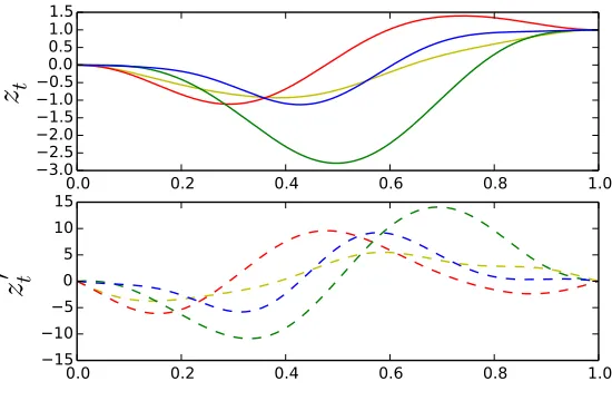
bothKa;aandK(a,b);(a,b)are indeed invertible because the kernel is assumed to be neither degenerate atanor degenerate atbgivena. Hence, the support of(za, za0, zb, z_b0)isR4, and any function and derivative values can be used for conditioning. Figure1illustrates example independent draws from aconditional derivative Gaussian process.

4. Or equivalently when the Gaussian vector(za, za)0 is degenerate.

3.1 String Gaussian Processes onR

The intuition behind string Gaussian processes on an interval comes from the analogy of collab-orative local GP experts we refer to as stringsthat are connected but independent of each other conditional on some regularity boundary conditions. While each string is tasked with representing local patterns in the data, a string only shares the states of its extremities (value and derivative) with adjacent strings. Our aim is to preserve global smoothness and limit the amount of informa-tion shared between strings, thus reducing computainforma-tional complexity. Furthermore, the condiinforma-tional independence between strings will allow for distributed inference, greater flexibility and principled nonstationarity construction.

The following theorem at the core of our framework establishes that it is possible to connect together GPs on a partition of an intervalI, in a manner consistent enough that the newly constructed stochastic object will be a stochastic process onI and in a manner restrictive enough that any two connected GPs will share just enough information to ensure that the constructed stochastic process is continuously differentiable (C1_{) onIin theL}2_sense.

Theorem 2 (String Gaussian process)

Leta0 <· · ·< ak <· · ·< aK,I = [a0, aK]and letpN(x;µ,Σ)be the multivariate Gaussian den-sity with mean vectorµand covariance matrixΣ. Furthermore, let(mk: [ak−1, ak]→ R)k∈[1..K]

be C1 _{functions, and(k}

k : [ak−1, ak]×[ak−1, ak] → R)k∈[1..K] be C3 symmetric positive

semi-definite functions, neither degenerate atak−1, nor degenerate atakgivenak−1.

(A) There exists anR2-valued stochastic process(SDt)t∈I, SDt= (zt, zt0)satisfying the following

conditions:

1) The probability density of(SDa0, . . . , SDaK)reads:

pb(x0, . . . , xK) := K

Y

k=0

pN

xk;µbk,Σbk

(5)

where: Σb₀=1Ka0;a0, ∀k >0 Σ b

k =kKak;ak −kKak;ak−1 kK

−1

ak−1;ak−1 kK T

ak;ak−1, (6)

µb₀ =1Ma0, ∀k >0 µ b

k=kMak +kKak;ak−1 kK

−1

ak−1;ak−1(xk−1−kMak−1), (7)

with _kKu;v =

"

kk(u, v) ∂k_∂yk(u, v) ∂kk

∂x(u, v) ∂2_k

k ∂x∂y(u, v)

#

, and _kMu =

mk(u) dmk

dt (u)

.

2) Conditional on(SDak =xk)k∈[0..K], the restrictions(SDt)t∈]ak−1,ak[, k∈[1..K]are

indepen-dent conditional derivative Gaussian processes, respectively with unconditional mean functionmk

and unconditional covariance functionkk and that are conditioned to take valuesxk−1 andxkat

ak−1 andakrespectively. We refer to(SDt)t∈Ias astring derivative Gaussian process, and to its

first coordinate(zt)t∈Ias astring Gaussian processnamely,

(zt)t∈I ∼ SGP({ak},{mk},{kk}).

(B) Thestring Gaussian process(zt)t∈Idefined in (A) isC1in theL2sense and itsL2derivative is

Proof SeeAppendix C.

In our collaborative local GP experts analogy, Theorem 2stipulates that each local expert takes as message from the previous expert its left hand side boundary conditions, conditional on which it generates its right hand side boundary conditions, which it then passes on to the next expert. Conditional on their boundary conditions local experts are independent of each other, and resemble vibrating pieces of string on fixed extremities, hence the namestring Gaussian process.

3.2 Pathwise Regularity

Thus far we have dealt with regularity only in the L2 _{sense. However, we note that a sufficient} condition for the process(z_t0)t∈Iin Theorem2to be almost surely continuous (i.e. sample paths are continuous with probability1) and to be the almost sure derivative of the string Gaussian process

(zt)t∈I, is that the Gaussian processes on Ik = [ak−1, ak] with mean and covariance functions

mak−1,ak ck andk

ak−1,ak

ck (as per Equations3and4withm:=mkandk:=kk) are themselves almost surelyC1 _{for every boundary condition.}6 _{We refer to (Adler and Taylor,2011, Theorem 2.5.2) for a} sufficient condition under which aC1_inL2_{Gaussian process is also almost surelyC}1_{. As the above} question is provably equivalent to that of the almost sure continuity of a Gaussian process (seeAdler and Taylor, 2011, p. 30), Kolmogorov’s continuity theorem(see Øksendal,2003, Theorem 2.2.3) provides a more intuitive, albeit stronger, sufficient condition than that of (Adler and Taylor,2011, Theorem 2.5.2).

3.3 Illustration

Algorithm1illustrates sampling jointly from a string Gaussian process and its derivative on an in-tervalI = [a0, aK]. We start off by sampling the string boundary conditions(zak, z

0

ak)sequentially, conditional on which we sample the values of the stochastic process on each string. This we may do in parallel as the strings are independent of each other conditional on boundary conditions. The resulting time complexity is the sum ofO(max n3_k)for sampling values within strings, andO(n)

for sampling boundary conditions, where the sample size isn=P

knk. The memory requirement grows as the sum of O(P

kn2k), required to store conditional covariance matrices of the values within strings, andO(K)corresponding to the storage of covariance matrices of boundary condi-tions. In the special case where strings are all empty, that is inputs and boundary times are the same, the resulting time complexity and memory requirement areO(n). Figure2illustrates a sample from a string Gaussian process, drawn using this approach.

3.4 String Gaussian Processes onRd

So far the input space has been assumed to be an interval. We generalise string GPs to hyper-rectangles inRdas stochastic processes of the form:

f(t1, . . . , td) =φ

z_t1₁, . . . , zd_td

, (10)

where thelink functionφ: Rd → Ris aC1function and(ztj)aredindependent (⊥) latent string Gaussian processes on intervals. We will occasionally refer tostring GPsindexed onRdwithd >1 asmembrane GPsto avoid any ambiguity. We note that whend = 1and when the link function

0.0 0.2 0.4 0.6 0.8 1.0 −3.0

−2.5 −2.0 −1.5 −1.0 −0.50.0 0.5 1.0 1.5

z

0.0 0.2 0.4 0.6 0.8 1.0

−15 −10 −5 0 5 10 15

z

′ t

Figure 1: Draws from a conditional derivative GP conditioned to start at 0 with derivative0and to finish at1.0with derivative0.0. The unconditional kernel is the squared exponential kernel with variance1.0and input scale0.2.

0.0 0.5 1.0 1.5 2.0 2.5 3.0

−4 −2 0 2 4 6 8

z

0.0 0.5 1.0 1.5 2.0 2.5 3.0

−100 −50 0 50 100

z

′ t

Algorithm 1Simulation of a string derivative Gaussian process

Inputs: boundary timesa0 <· · ·< aK, string times{tkj ∈]ak−1, ak[}j∈[1..nk],k∈[1..K], uncondi-tional mean (resp. covariance) functionsmk(resp.kk)

Output: {. . . , zak, z

0

ak, . . . , ztk_j, z

0

tk j

, . . .}.

Step 1: sample the boundary conditions sequentially. fork= 0toKdo

Sample(zak, z

0

ak)∼ N

µb_k,Σb_k, withµb_kandΣb_kas per Equations (7) and (6). end for

Step 2: sample the values on each string conditional on the boundary conditions inparallel. parfork= 1toKdo

LetkMuandkKu;vbe as in Theorem2,

kΛ =



 

kKtk

1;ak−1 kKtk1;ak

. . . .

kKtk

nk;ak−1 kKtk_nk;ak



 

kKak−1;ak−1 kKak−1;ak kKak;ak−1 kKak;ak

−1

,

µs_k=



 

kMtk 1

. . .

kMtk nk





+kΛ



  

zak−1 −mk(ak−1)

z0_ak−1 −dmk dt (ak−1)

zak−mk(ak)

z0_a

k − dmk

dt (ak)



  

, (8)

Σs_k =



 

kKtk

1;tk1 . . . kKtk1;tknk

. . . .

kKtk

nk;tk1 . . . kKtknk;tknk





−kΛ



 

kKtk

1;ak−1 kKtk1;ak

. . . .

kKtk

nk;ak−1 kKtk_nk;ak



 

T

. (9)

Sample

z_tk 1, z

0

tk 1

. . . , z_tk nk, z

0

tk nk

∼ N(µs_k,Σs_k).

isφ(x) = x, we recoverstring GPsindexed on an interval as previously defined. When thestring GPs(z_tj)are a.s.C1_{, themembrane GPf in Equation (10) is also a.s.C}1_{, and the partial derivative} with respect to thej-th coordinate reads:

∂f ∂tj

(t1, . . . , td) =ztjj0

∂φ ∂tj

z_t1₁, . . . , z_td

d

. (11)

Thus in high dimensions, string GPseasily allow an explanation of the sensitivity of the learned latent function to inputs.

3.5 Choice of Link Function

Our extension of string GPs to Rd departs from the standard GP paradigm in that we did not postulate a covariance function onRd×Rd directly. Doing so usually requires using a metric on Rd, which is often problematic for heterogeneous input dimensions, as it introduces an arbitrary comparison between distances in each input dimension. This problem has been partially addressed by approaches such as Automatic Relevance Determination (ARD) kernels, that allow for a lin-ear rescaling of input dimensions to be llin-earned jointly with kernel hyper-parameters. However, inference under astring GPprior can be thought of as learning a coordinate system in which the latent function f resembles the link functionφthrough non-linear rescaling of input dimensions. In particular, whenφis symmetric, the learned univariatestring GPs(being interchangeable inφ) implicitly aim at normalizing input data across dimensions, makingstring GPsnaturally cope with heterogeneous data sets.

An important question arising from our extension is whether or not the link functionφneeds to be learned to achieve a flexible functional prior. The flexibility of astring GPas a functional prior depends on both thelink functionand the covariance structures of the underlyingstring GPbuilding blocks(z_tj). To address the impact of the choice of φ on flexibility, we constrain thestring GP

building blocks by restricting them to be independent identically distributedstring GPswith one string each (i.e. (zj_t)are i.i.d Gaussian processes). Furthermore, we restrict ourselves to isotropic kernels as they provide a consistent basis for putting the same covariance structure in RandRd. One question we might then ask, for a given link functionφ0, is whether or not an isotropic GP indexed onRdwith covariance functionkyields more flexible random surfaces than the stationary

string GPf(t1, . . . , td) = φ0(zt11, . . . , z d

td), where(z j

tj)are stationary GPs indexed onRwith the same covariance functionk. If we find alink functionφ0generating more flexible random surfaces than isotropic GP counterparts it would suggestφneed not to be inferred in dimensiond > 1to be more flexible than any GP using one of the large number of commonly used isotropic kernels, among which squared exponential kernels, rational quadratic kernels, and Mat´ern kernels to name but a few.

Before discussing whether such aφ0 exists, we need to introduce a rigorous meaning to ‘flexi-bility’. An intuitive qualitative definition of the flexibility of a stochastic process indexed onRdis the ease with which it can generate surfaces with varying shapes from one random sample to another independent one. We recall that the tangent hyperplane to aC1 _{surfacey−f(x) = 0, x ∈}

Rdat some pointx0 = (t01, . . . , t0d)has equation∇f(x0)T(x−x0)−(y−f(x0)) = 0and admits as nor-mal vector(_∂t∂f

1(t 0 1), . . . ,

∂f ∂td(t

0

This criterion alone, however, does not capture the difference between the local shapes of the ran-dom surface at two distinct points. A complementary second criterion of flexibility is the proclivity of the (random) directions of the tangent hyperplanes at any two distinct pointsx0, x1 ∈Rd—and hence the proclivity of∇f(x0)and∇f(x1)—to be independent. The first criterion can be measured using the entropy of the gradient at a point, while the second criterion can be measured through the mutual information between the two gradients. The more flexible a stochastic process, the higher the entropy of its gradient at any point, and the lower the mutual information between its gradients at any two distinct points. This is formalised in the definition below.

Definition 3 (Flexibility of stochastic processes)

Letf andgbe two real valued, almost surelyC1 _{stochastic processes indexed on}

Rd, and whose

gradients have a finite entropy everywhere (i.e. ∀x, H(∇f(x)), H(∇g(x))<∞). We say thatf

is more flexible thangif the following conditions are met: 1)∀x, H(∇f(x))≥H(∇g(x)),

2)∀x6=y, I(∇f(x);∇f(y))≤I(∇g(x);∇g(y)),

whereHis the entropy operator, andI(X;Y) =H(X) +H(Y)−H(X, Y)stands for the mutual information betweenXandY.

The following proposition establishes that thelink functionφs(x1, . . . , xd) =

Pd

i=jxjyields more flexible stationarystring GPsthan their isotropic GP counterparts, thereby providing a theoretical underpinning for not inferringφ.

Proposition 4 (Additively separablestring GPsare flexible)

Letk(x, y) :=ρ ||x−y||2 L2

be a stationary covariance function generating a.s. C1 _{GP paths}

in-dexed onRd, d >0, andρa function that isC2on]0,+∞[and continuous at0. Letφs(x1, . . . , xd) =

Pd

j=1xj, let(z j

t)t∈Ij_{, j∈[1..d]} be independent stationary Gaussian processes with mean0and

co-variance functionk(where theL2 norm is on_R), and letf(t1, . . . , td) = φs(z1t1, . . . , z d

td) be the

corresponding stationary string GP. Finally, let g be an isotropic Gaussian process indexed on

I1_{× · · · ×I}d_{with mean 0 and covariance functionk(where theL}2_{norm is on}

Rd). Then:

1)∀x∈I1× · · · ×Id, H(∇f(x)) =H(∇g(x)),

2)∀x6=y∈I1_{× · · · ×I}d_{, I(∇f(x);∇f(y))≤I(∇g(x);∇g(y)).}

Proof SeeAppendix E.

Although the link function need not be inferred in a full nonparametric fashion to yield compara-ble if not better results than most isotropic kernels used in the standard GP paradigm, for some problems certain link functions might outperform others. In Section4.2we analyse a broad family of link functions, and argue that they extend successful anisotropic approaches such as the Au-tomatic Relevance Determination (MacKay (1998)) and the additive kernels of Duvenaud et al.

(2011). Moreover, in Section 5 we propose a scalable inference scheme applicable to any link function.

4. Comparison with the Standard GP Paradigm

We have already established that samplingstring GPs scales better than sampling GPs under the

stationary additively separablestring GPsare more flexible than their isotropic counterparts in the

standard GP paradigm. In this section, we provide further theoretical results relating the string GP paradigmto thestandard GP paradigm. Firstly we establish thatstring GPswith link function

φs(x1, . . . , xd) =Pdi=jxj are GPs. Secondly, we derive the global mean and covariance functions induced by thestring GPconstruction for a variety of link functions. Thirdly, we provide a sense in which thestring GP paradigmcan be thought of as extending thestandard GP paradigm. And finally, we show that thestring GP paradigmmay serve as a scalable approximation of commonly used stationary kernels.

4.1 Some String GPs are GPs

On one hand we note from Theorem2that the restriction of astring GPdefined on an interval to the support of the first string—in other words the first local GP expert—is a Gaussian process. On the other hand, the messages passed on from one local GP expert to the next are not necessarily consistent with the unconditional law of the receiving local expert, so that overall a string GP

defined on an interval, that is when looked at globally and unconditionally, might not be a Gaussian process. However, the following proposition establishes that somestring GPsare indeed Gaussian processes.

Proposition 5 (Additively separablestring GPsare GPs)

String Gaussian processes on_Rare Gaussian processes. Moreover, string Gaussian processes on

Rdwith link functionφs(x1, . . . , xd) =Pdj=1xj are also Gaussian processes.

Proof The intuition behind this proof lies in the fact that if X is a multivariate Gaussian, and if conditional onX,Y is a multivariate Gaussian, providing that the conditional mean ofY depends linearly onXand the conditional covariance matrix ofY does not depend onX, the vector(X, Y)

is jointly Gaussian. This will indeed be the case for our collaboration of local GP experts as the boundary conditions picked up by an expert from the previous will not influence the conditional co-variance structure of the expert (the conditional coco-variance strucuture depends only on the partition of the domain, not the values of the boundary conditions) and will affect the mean linearly. See Appendix Hfor the full proof.

The above result guarantees that commonly used closed form predictive equations under GP priors are still applicable under somestring GPpriors, providing the global mean and covariance functions, which we derive in the following section, are available. Proposition 5also guarantees stability of the correspondingstring GPsin the GP family under addition of independent Gaussian noise terms as in regression settings. Moreover, it follows from Proposition5that inference tech-niques developed for Gaussian processes can be readily used understring GPpriors. In Section5 we provide an additional MCMC scheme that exploits the conditional independence between strings to yield greater scalability and distributed inference.

4.2 String GP Kernels and String GP Mean Functions

models under the standard GP paradigm, which would provide a flexible and nonstationary al-ternative to commonly used kernels that may be used to learn local patterns in data sets—some successful example applications are provided in Section5. That being said, adopting such a global approach should be limited to small scale problems as the conditional independence structure of

string GPs does not easily translate into structures in covariance matrices overstring GP values (without derivative information) that can be exploited to speed-up SVD or Cholesky decomposi-tion. Crucially, marginalising out all derivative information in the distribution ofderivative string GPvalues at some inputs would destroy any conditional independence structure, thereby limiting opportunities for scalable inference. In Section5we will provide a RJ-MCMC inference scheme that fully exploits the conditional independence structure instring GPsand scales tovery largedata sets.

4.3 Connection Between Multivariate String GP Kernels and Existing Approaches

We recall that forn ≤ d, then-th orderelementary symmetric polynomial(Macdonald(1995)) is given by

e0(x1, . . . , xd) := 1, ∀1≤n≤d en(x1, . . . , xd) =

X

1≤j1<j2<···<jn≤d n

Y

k=1

xjk. (12)

As an illustration,

e1(x1, . . . , xd) = d

X

j=1

xj =φs(x1, . . . , xd),

e2(x1, . . . , xd) =x1x2+x1x3+· · ·+x1xd+· · ·+xd−1xd,

. . .

ed(x1, . . . , xd) = d

Y

j=1

xj =φp(x1, . . . , xd).

Covariance kernels ofstring GPs, using as link functions elementary symmetric polynomials en, extend most popular approaches that combine unidimensional kernels over features for greater flex-ibility or cheaper design experiments.

The first-order polynomiale1 gives rise to additively separable Gaussian processes, that can be regarded as Bayesian nonparametricgeneralised additive models(GAM), particularly popular for their interpretability. Moreover, as noted byDurrande et al.(2012), additively separable Gaussian processes are considerably cheaper than alternate transformations in design experiments with high-dimensional input spaces. In addition to the above, additively separable string GPs also allow postulating the existence of local properties in the experimental design process at no extra cost.

The d-th order polynomialedcorresponds to a product of unidimensional kernels, also known as separable kernels. For instance, the popular squared exponential kernel is separable. Separable kernels have been successfully used on large scale inference problems where the inputs form a grid (Saatchi,2011;Wilson et al.,2014), as they yield covariance matrices that are Kronecker products, leading to maximum likelihood inference in linear time complexity and with linear memory require-ment. Separable kernels are often used in conjunction with theautomatic relevance determination

kernels might be limited in that we might want the relevance of a feature to depend on its value. As an illustration, the market value of a watch can be expected to be a stronger indicator of its owner’s wealth when it is in the top 1 percentile, than when it is in the bottom 1 percentile; the rationale being that possessing a luxurious watch is an indication that one can afford it, whereas possessing a cheap watch might be either an indication of lifestyle or an indication that one cannot afford a more expensive one. Separablestring GPkernels extend ARD kernels, in that strings between input dimensions and within an input dimension may have unconditional kernels with different hyper-parameters, and possibly different functional forms, thereby allowing forautomatic local relevance determination(ALRD).

More generally, using as link function the n-th order elementary symmetric polynomial en corresponds to then-th order interaction of the additive kernels ofDuvenaud et al. (2011). We also note that the class of link functionsφ(x1, . . . , xd) =

Pd

i=1σiei(x1, . . . , xd)yield fulladditive

kernels.Duvenaud et al.(2011) noted that such kernels are ‘exceptionally well-suited’ to learn non-local structures in data. String GPscomplementadditive kernels by allowing them to learn local structures as well.

4.4 String GPs as Extension of the Standard GP Paradigm

The following proposition provides a perspective from which string GPs may be considered as extending Gaussian processes on an interval.

Proposition 6 (Extension of thestandard GP paradigm)

LetK ∈_N∗, letI = [a0, aK]andIk = [ak−1, ak]be intervals witha0 <· · ·< aK. Furthermore,

let m : I → _Rbe aC1 _function,m

k the restriction ofm toIk, h : I ×I → Ra C3 symmetric

positive semi-definite function, andhkthe restriction ofhtoIk×Ik. If

(zt)t∈I ∼ SGP({ak},{mk},{hk}),

then

∀k∈[1..K], (zt)t∈Ik ∼ GP(m, h).

Proof SeeAppendix F.

We refer to the case where unconditional string mean and kernel functions are restrictions of the same functions as in Proposition6 asuniform string GPs. Although uniformstring GPsare not guaranteed to be as much regular at boundary times as their counterparts in thestandard GP paradigm, we would like to stress that they may well generate paths that are. In other words, the functional space induced by a uniformstring GPon an interval extends the functional space of the GP with the same mean and covariance functionsmandhtaken globally and unconditionally on the whole interval as in the standard GP paradigm. This allows for (but does not enforce) less regularity at the boundary times. Whenstring GPsare used as functional prior, the posterior mean can in fact have more regularity at the boundary times than the continuous differentiability enforced in thestring GP paradigm, providing such regularity is evidenced in the data.

We note from Proposition6 that whenmis constant and his stationary, the restriction of the uniform string GP (zt)t∈I to any interval whose interior does not contain a boundary time, the largest of which being the intervals[ak−1, ak], is a stationary GP. We refer to such cases aspartition

4.5 Commonly Used Covariance Functions and their String GP Counterparts

Considering the superior scalability of thestring GP paradigm, which we may anticipate from the scalability of samplingstring GPs, and which we will confirm empirically in Section 5, a natural question that comes to mind is whether or not kernels commonly used in thestandard GP paradigm

can be well approximated bystring GPkernels, so as to take advantage of the improved scalability of the string GP paradigm. We examine the distortions to commonly used covariance structures resulting from restricting strings to share only C1 _{boundary conditions, and from increasing the} number of strings.

Figure3compares some popular stationary kernels on[0,1]×[0,1](first column) to their uni-formstring GP kernel counterparts with 2, 4, 8 and 16 strings of equal length. The popular ker-nels considered are the squared exponential kernel (SE), the rational quadratic kernelkRQ(u, v) =

1 +2(u−_αv)2

−α

5. Inference under String and Membrane GP Priors

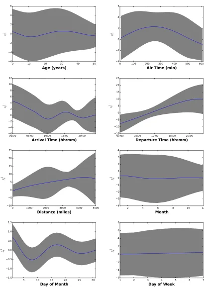
In this section we move on to developing inference techniques for Bayesian nonparametric inference of latent functions understring GPpriors. We begin with marginal likelihood inference in regression problems. We then propose a novel reversible-jump MCMC sampler that enables automatic learning of model complexity (that is the number of different unconditional kernel configurations) from the data, with a time complexity and memory requirement both linear in the number of training inputs.

5.1 Maximum Marginal Likelihood for Small Scale Regression Problems

Firstly, we leverage the fact that additively separablestring GPsare Gaussian processes to perform Bayesian nonparametric regressions in the presence of local patterns in the data, using standard Gaussian process techniques (seeRasmussen and Williams,2006, p.112§5.4.1). We use as genera-tive model

yi=f(xi) +i, i ∼ N 0, σk2i

, σ_k2_i >0, xi ∈I1× · · · ×Id, yi, i∈R

we are given the training data setD={x˜i,y˜i}i∈[1..N],and we place a mean-zero additively separa-blestring GPprior onf, namely

f(x) =

d

X

j=1

zj_x[j], (z_tj)∼ SGP{aj_k},{0},{k_kj}, ∀j < l, (z_tj)⊥(zl_t),

which we assume to be independent of the measurement noise process. Moreover, the noise terms are assumed to be independent, and the noise variance σ2_k

i affectingf(xi) is assumed to be the same for any two inputs whose coordinates lie on the same string intervals. Such a heteroskedastic noise model fits nicely within thestring GP paradigm, can be very useful when the dimension of the input space is small, and may be replaced by the typical constant noise variance assumption in high-dimensional input spaces.

Let us definey = (˜y1, . . . ,y˜N),X= (˜x1, . . . ,x˜N),f = (f(˜x1), . . . , f(˜xN))and letK¯X;X

de-note the auto-covariance matrix off(which we have derived in Section4.2), and letD=diag({σ_k2

i}) denote the diagonal matrix of noise variances. It follows thatyis a Gaussian vector with mean 0 and auto-covariance matrixKy:= ¯KX;X+Dand that the log marginal likelihood reads:

logpy

X,{σki},{θ j k},{a

j k}

=−1

2y

T_K−1

y y− 1

2logdet(Ky)−

n

2 log 2π. (13)

We obtain estimates of the string measurement noise standard deviations{σˆki}and estimates of the string hyper-parameters{θˆ_kj}by maximising the marginal likelihood for a given domain partition

{aj_k}, using gradient-based methods. We deduce the predictive mean and covariance matrix of the latent function valuesf∗at test pointsX∗, from the estimates{θˆ_kj},{σˆki}as

E(f∗|y) = ¯KX∗;XK−y1y and cov(f

∗_|

y) = ¯KX∗;X∗−K¯X∗;XK−y1K¯X;X∗, (14)

5.1.1 REMARKS

The above analysis and equations still hold when a GP prior is placed onf with one of the multi-variatestring GPkernels derived in Section4.2as covariance function.

It is also worth noting from the derivation ofstring GPkernels inAppendix Ithat the marginal likelihood Equation (13) is continuously differentiable in the locations of boundary times. Thus, for a given number of boundary times, the positions of the boundary times can be determined as part of the marginal likelihood maximisation. The derivatives of the marginal log-likelihood (Equation 13) with respect to the aforementioned locations {aj_k} can be determined from the recursions of Appendix I, or approximated numerically by finite differences. The number of boundary times in each input dimension can then be learned by trading off model fit (the maximum marginal log likelihood) and model simplicity (the number of boundary times or model parameters), for instance using information criteria such as AIC and BIC. When the input dimension is large, it might be advantageous to further constrain the hypothesis space of boundary times before using information criteria, for instance by assuming that the number of boundary times is the same in each dimension. An alternative Bayesian nonparametric approach to learning the number of boundary times will be discussed in section5.4.

This method of inference cannot exploit the structure ofstring GPsto speed-up inference, and as a result it scales like thestandard GP paradigm. In fact, any attempt to marginalize out univariate derivative processes, including in the prior, will inevitably destroy the conditional independence structure. Another perspective to this observation is found by noting from the derivation of global

string GPcovariance functions inAppendix Ithat the conditional independence structure does not easily translate in a matrix structure that may be exploited to speed-up matrix inversion, and that marginalizing out terms relating to derivatives processes as in Equation (13) can only make things worse.

5.2 Generic Reversible-Jump MCMC Sampler for Large Scale Inference

More generally, we consider learning a smooth real-valued latent function f, defined on a d -dimensional hyper-rectangle, under a generative model with likelihoodp(D|f,u), wheref denotes values of f at training inputs points and u denotes other likelihood parameters that are not re-lated tof. A large class of machine learning problems aiming at inferring a latent function have a likelihood model of this form. Examples include celebrated applications such as nonparametric re-gression and nonparametric binary classification problems, but also more recent applications such as learning a profitable portfolio generating-function instochastic portfolio theory(Karatzas and Fern-holz(2009)) from the data. In particular, we do not assume thatp(D|f,u)factorizes over training inputs. Extensions to likelihood models that depend on the values of multiple latent functions are straight-forward and will be discussed in Section5.3.

5.2.1 PRIORSPECIFICATION

We place a priorp(u)on other likelihood parameters. For instance, in regression problems under a Gaussian noise model,u can be the noise variance and we may choosep(u)to be the inverse-Gamma distribution for conjugacy. We place a mean-zerostring GPprior onf

f(x) =φ

z1_x[1], . . . , z_xd_[d]

As discussed in Section3.5, the link function φneed not be inferred as the symmetric sum was found to yield a sufficiently flexible functional prior. Nonetheless, in this section we do not impose any restriction on the link functionφother than continuous differentiability. Denotingzthe vector of univariate string GP processes and their derivatives, evaluated at all distinct input coordinate values, we may re-parametrize the likelihood asp(D|z,u), with the understanding thatf can be recovered from z through the link function φ. To complete our prior specification, we need to discuss the choice of boundary times{aj_k}and the choice of the corresponding unconditional kernel structures{kj_k}. Before doing so, we would like to stress that key requirements of our sampler are that i) it should decouple the need for scalability from the need for flexibility, ii) it should scale linearly with the number of training and test inputs, and iii) the user should be able to express prior views on model complexity/flexibility in an intuitive way, but the sampler should be able to validate or invalidate the prior model complexity from the data. While the motivations for the last two requirements are obvious, the first requirement is motivated by the fact that a massive data set may well be more homogeneous than a much smaller data set.

5.2.2 SCALABLECHOICE OFBOUNDARYTIMES

To motivate our choice of boundary times that achieves great scalability, we first note that the evaluation of the likelihood, which will naturally be needed by the MCMC sampler, will typically have at least linear time complexity and linear memory requirement, as it will require performing computations that use each training sample at least once. Thus, the best we can hope to achieve overall is linear time complexity and linear memory requirement. Second, in MCMC schemes with functional priors, the time complexity and memory requirements for sampling from the posterior

p(f|D)∝p(D|f)p(f)

are often the same as the resource requirements for sampling from the prior p(f), as evaluating the model likelihood is rarely the bottleneck. Finally, we note from Algorithm1that, when each input coordinate in each dimension is a boundary time, the sampling scheme has time complexity and memory requirement that are linear in the maximum number of unique input coordinates across dimensions, which is at most the number of training samples. In effect, each univariate derivative

string GPis sampled inparallelat as many times as there are unique input coordinates in that di-mension, before being combined through the link function. In a given input didi-mension, univariate

derivative string GPvalues are sampled sequentially, one boundary time conditional on the previ-ous. The foregoing sampling operation is very scalable not only asymptotically but also in absolute terms; it merely requires storing and inverting at most as many 2×2matrices as the number of input points. We will evaluate the actual overall time complexity and memory requirement when we discuss our MCMC sampler in greater details. For now, we would like to stress that i) choosing each distinct input coordinate value as a boundary time in the corresponding input dimension before training is a perfectly valid choice, ii) we expect this choice to result in resource requirements that grow linearly with the sample size and iii) in thestring GPtheory we have developed thus far there is no requirement that two adjacent strings be driven by different kernel hyper-parameters.

5.2.3 MODELCOMPLEXITYLEARNING AS ACHANGE-POINTPROBLEM

setup departs from postulating the unconditional string covariance function k_kj globally similarly to the standard GP paradigm. The more distinct unconditional covariance structures there are, the more complex the model is, as it may account for more types of local patterns. Thus, we may identify model complexity to the number of different kernel configurations across input dimensions. In order to learn model complexity, we require that some (but not necessarily all) strings share their kernel configuration.7 Moreover, we require kernel membership to be dimension-specific in that two strings in different input dimensions may not explicitly share a kernel configuration in the prior specification, although the posterior distribution over their hyper-parameters might be similar if the data support it.

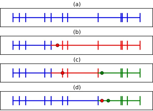
In each input dimension j, kernel membership is defined by a partition of the corresponding domain operated by a (possibly empty) set of change-points,8as illustrated in Figure4. When there is no change-point as in Figure4-(a), all strings are driven by the same kernel and hyper-parameters. Each change-point cjp induces a new kernel configuration θpj that is shared by all strings whose boundary times aj_k andaj_k+1 both lie in[cjp, cjp+1[. When one or multiple change-pointsc

j p occur between two adjacent boundary times as illustrated in Figures4-(b-d), for instanceaj_k≤cjp ≤aj_k+1, the kernel configuration of the string defined on[aj_k, aj_k+1]is that of the largest change-point that lies in[aj_k, aj_k+1](see for instance Figure4-(d)). For consistency, we denoteθj₀the kernel configuration driving the first string in thej-th dimension; it also drives strings that come before the first change-point, and all strings when there is no change-point.

To place a prior on model complexity, it suffices to define a joint probability measure on the set of change-points and the corresponding kernel configurations. As kernel configurations are not shared across input dimensions, we choose these priors to be independent across input dimen-sions. Moreover,{cjp}being a random collection of points on an interval whose number and po-sitions are both random, it isde factoa point process (Daley and Vere-Jones(2008)). To keep the prior specification of change-points uninformative, it is desirable that conditional on the number of change-points, the positions of change-points be i.i.d. uniform on the domain. As for the number of change-points, it is important that the support of its distribution not be bounded, so as to allow for an arbitrarily large model complexity if warranted. The two requirements above are satisfied by a homogeneous Poisson process or HPP (Daley and Vere-Jones(2008)) with constant intensityλj. More precisely, the prior probability measure on

{cjp, θjp}, λj

is constructed as follows:



    

    

λj ∼Γ(αj, βj),

{cjp}

λj ∼HPP(λj)

θjp[i]

{c

j

p}, λj i.i.d∼ logN(0, ρj)

∀(j, p)6= (l, q)θjp ⊥θlq,

, (16)

where we choose the Gamma distributionΓas prior on the intensityλjfor conjugacy, we assume all kernel hyper-parameters are positive as is often the case in practice,9the coordinates of the hyper-parameters of a kernel configuration are assumed i.i.d., and kernel hyper-hyper-parameters are assumed

7. That is, the functional form of the unconditional kernelkj_kand its hyper-parameters.

8. We would like to stress that change-points do not introduce new input points or boundary times, but solely define a partition of the domain of each input dimension.

(a)

(b)

(c)

(d)

independent between kernel configurations. Denoting the domain of thej-th input[aj, bj], it follows from applying the laws of total expectation and total variance on Equation (16) that the expected number of change-points in thej-th dimension under our prior is

E #{cj_p}

= bj−ajα

j

βj, (17)

and the variance of the number of change-points in thej-dimension under our prior is

Var #{cj_p}

= bj −ajα

j

βj 1 +

bj−aj

βj

!

. (18)

The two equations above may guide the user when setting the parametersαj _andβj_{. For instance,} these values may be set so that the expected number of change-points in a given input dimension be a fixed fraction of the number of boundary times in that input dimension, and so that the prior variance over the number of change-points be large enough that overall the prior isn’t too informative.

We could have taken a different approach to construct our prior on change-points. In effect, assuming for the sake of the argument that the boundaries of the domain of thej-th input, namely

aj_andbj_{, are the first and last change-point in that input dimension, we note that the mapping}

. . . , cj_p, . . .→ . . . , pj_p, . . .:= . . . ,c

j p+1−c

j p

bj_−aj , . . .

!

defines a bijection between the set of possible change-points in the j-th dimension and the set of all discrete probability distributions. Thus, we could have placed as prior on . . . , pjp, . . .

a Dirichlet process (Ferguson(1973)), a Pitman-Yor process (Pitman and Yor(1997)), more generally

normalized completely random measures (Kingman (1967)) or any other probability distribution over partitions. We prefer the point process approach primarily because it provides an easier way of expressing prior belief about model complexity through the expected number of change-points

#{cjp}, while remaining uninformative about positions thereof.

One might also be tempted to regard change-points in an input dimensionj as inducing a par-tition, not of the domain [aj_{, b}j_{], but of the set of boundary times a}j

augmented spaces, which makes this choice of prior specification somewhat similar, but stronger (that is more informative) than the one we adopt in this paper.

Before deriving the sampling algorithm, it is worth noting that the prior defined in Equation (16) does not admit a density with respect to the same base measure,10as the number of change-points

#{cjp}, and subsequently the number of kernel configurations, may vary from one sample to another. Nevertheless, the joint distribution over the dataDand all other model parameters is well defined and, as we will see later, we may leverage reversible-jump MCMC techniques (Green(1995);Green and Hastie(2009)) to construct a Markov chain that converges to the posterior distribution.

5.2.4 OVERALLSTRUCTURE OF THEMCMC SAMPLER

To ease notations, we denote c the set of all change-points in all input dimensions, we denote

n=. . . ,#{cjp}, . . .

∈_Nd_{the vector of the numbers of change-points in each input dimension,}

we denoteθthe set of kernel hyper-parameters,11andρ:= (. . . , ρj_{, . . .)the vector of variances of} the independent log-normal priors onθ. We denoteλ:= (. . . , λj, . . .)the vector of change-points intensities, we denoteα := (. . . , αj, . . .)andβ := (. . . , βj, . . .)the vectors of parameters of the Gamma priors we placed on the change-points intensities across thedinput dimensions, and we recall thatudenotes the vector of likelihood parameters other than the values of the latent function

f.

We would like to sample from the posterior distributionp(f,f∗,∇f,∇f∗|D,α,β,ρ), wheref andf∗are the vectors of values of the latent functionf at training and test inputs respectively, and

∇f,∇f∗the corresponding gradients. Denotingzthe vector of univariatestring GPprocesses and their derivatives, evaluated at all distinct training and test input coordinate values, we note that to sample from p(f,f∗,∇f,∇f∗|D,α,β,ρ), it suffices to sample from p(z|D,α,β,ρ), computef andf∗ using the link function, and compute the gradients using Equation (11). To sample from

p(z|D,α,β,ρ), we may sample from the target distribution

π(n,c,θ,λ,z,u) :=p(n,c,θ,λ,z,u|D,α,β,ρ), (19)

and discard variables that are not of interest. As previously discussed,πis not absolutely continuous with respect to the same base measure, though we may still decompose it as

π(n,c,θ,λ,z,u) = 1

p(D|α,β,ρ)p(n|λ)p(λ|α,β)p(c|n)p(θ|n,ρ)p(u)p(z|c,θ)p(D|z,u),

(20) where we use the notation p(.) and p(.|.) to denote probability measures rather than probability density functions or probability mass functions, and where product and scaling operations are usual measure operations. Before proceeding any further, we will introduce a slight re-parametrization of Equation (20) that will improve the inference scheme.

Letna = (. . . ,#{ajk}k, . . .)be the vector of the numbers of unique boundary times in alld input dimensions. We recall from our prior onfthat

p(z|c,θ) =

d

Y

j=1

p

zj

aj₀, z j0

aj₀

na[j]−1 Y

k=1

p

zj

aj_k, z j0

aj_k

z

j aj_k−1, z

j0

aj_k−1

, (21)

10. That is the joint prior probability measure is neither discrete, nor continuous.

where each factor in the decomposition above is a bivariate Gaussian density whose mean vector and covariance matrix is obtained from the partitionsc, the kernel hyper-parametersθ, and the kernel membership scheme described in Section 5.2.3 and illustrated in Figure4, and using Equations (6-7). Let j_kKu;v be the unconditional covariance matrix between

zuj, zuj0

and

zvj, zjv0

as per

the unconditional kernel structure driving the string defined on the interval[aj_k, aj_k+1[. LetΣj₀ :=

j

0Kaj₀;aj₀ be the auto-covariance matrix of

zj

aj₀, z j0

aj₀

. Let

Σj_k:=j_kK_aj

k;a j k

−j_kK_aj k;a

j k−1

j kK

−1 aj_k−1;aj_k−1

j kK

T aj_k;aj_k−1

be the covariance matrix of

zj

aj_k, z j0

aj_k

given

zj

aj_k−1

, zj0

aj_k−1

, and

M_kj =j_kK_aj k;a

j k−1

j kK

−1 aj_k−1;aj_k−1.

Finally, letLj_k := U_kj(Dj_k)12 withΣj k = U

j kD

j k(U

j

k)T the singular value decomposition (SVD) of

Σj_k. We may choose to represent

zj

aj₀, z j0

aj₀

as





zj

aj₀

zj0

aj0



=L

j 0x

j

0, (22)

and fork >0we may also choose to represent

zj

aj_k, z j0

aj_k

as





zj

aj_k

zj0

aj_k



=M

j k





zj

aj_k−1

zj0

aj_k−1



+L

j kx

j

k, (23)

where{xj_k}are independent bivariate standard normal vectors. Equations (22-23) provide an equiv-alent representation. In effect, we recall that ifZ = M+LX,whereX ∼ N(0, I)is a standard multivariate Gaussian,M is a real vector, andLis a real matrix, thenZ∼ N(M, LLT). Equations

(22-23) result from applying this result to

zj

aj0

, zj0

aj0

and

zj

aj_k, z j0

aj_k

zj

aj_k−1

, zj0

aj_k−1

. We note

that at training time,M_kjandLj_konly depend on kernel hyper-parameters. Denotingxthe vector of allxj_k,xis a so-called ‘whitened’ representation ofz, which we prefer for reasons we will discuss shortly. In the whitened representation, the target distributionπis re-parameterized as

π(n,c,θ,λ,x,u) = 1

p(D|α,β,ρ)p(n|λ)p(λ|α,β)p(c|n)p(θ|n,ρ)p(u)p(x)p(D|x,c,θ,u),