Reaction Function Model of Monetary Policy under Inflation Targeting Framework in Indonesia

(1)

ISSN: 2306-9007 Adenan (2014) 211

I

www.irmbrjournal.com March 2014

I

nternational

R

eview of

M

anagement and

B

usiness

R

esearch

Vol. 3 Issue.1

R

M

B

R

Reaction Function Model of Monetary Policy under

Inflation Targeting Framework in Indonesia

MOH ADENAN

Faculty of Economics University of Jember, Indonesia Jl. Kalimantan No. 37 Jember 68121 Telp. 0331-337990

Fax. 0331-332150 HP: 062- 81559-222-18

Email: [email protected]

Abstract

The study aimed were 1. to test and analyze real GDP lag, real GDP lead, real interest rate and real exchange rate simultaneously and partially affected on output gap; 2. to test and analyze real GDP and SBI interest rate simultaneously and partially affected on real money balance; 3. to test and analyze inflation lead, inflation lag, real GDP lag, real exchange rate lag, real exchange rate lag 2 simultaneously and partially affected on inflation; 4. to test and analyze output gap and inflation gap simultaneously and partially affected on SBI interest rate; 5. to test and analyze output gap, inflation gap and real exchange rate gap simultaneously and partially affected on SBI interest rate; and then 6. to describe reaction function model of opened economy was better than model of closed economy. The study concluded that 1. real GDP lag, real GDP lead, real interest rate and real exchange rate simultaneously significant affected on output gap. Real GDP lag, real interest rate and real exchange rate partially significant affected on output gap, but real GDP lead did not; 2. real GDP and SBI interest rate simultaneously and partially significant affected on real money balance; 3. inflation lead, inflation lag, real GDP lag, real exchange rate lag and real exchange rate lag 2 simultaneously significant affected on inflation. Inflation lead, inflation lag and real GDP lag partially significant affected on inflation, but real exchange rate lag and real exchange rate lag 2 did not; 4. output gap and inflation gap simultaneously significant affected on SBI interest rate. Inflation gap partially significant affected on SBI interest rate, but output gap did not; 5. output gap, inflation gap and real exchange rate gap simultaneously significant affected on SBI interest rate. Inflation gap partially significant affected on SBI interest rate, but output gap and exchange rate gap did not; then 6. reaction function model of opened economy was better than closed economy one, proven that value of social welfare loss function of opened economy model less than value of closed one. Contributions of the study were 1. to enlarge alternative reaction function model of monetary policy; and 2. to prove that both reaction function models needed discretion more than rule considering of low determinant coefficient. Based on the study, it was recommended that: 1. BI should adopt reaction function model of opened economy in formulating the following monetary policy; 2. BI should focused on achieving inflation target through utilizing five pillars policy mix related the study, as follows consistent monetary policy to achieve inflation target, exchange rate policy to control stability of rupiah and communication strategy to support effectiveness of policy; and 3. BI should revitalize monetary instrument of discount window to regulate banking and control low inflation rate.

Key Words: Monetary Policy, Reaction Function Model and Inflation Targeting.

Introduction

(2)

ISSN: 2306-9007 Adenan (2014) 212

I

nternational

R

eview of

M

anagement and

B

usiness

R

esearch

Vol. 3 Issue.1

R

M

B

R

of Inflation Targeting (IT) in developed and industrializing countries was success in decreasing inflation rate. It could be seen in New Zealand, Australian, Canada, Sweden, Great Britain, Norway, Swiss, Finland and Spain, Brazil, Chile, Colombian, Cekoslowakia Republics, Hongary, Israel, South Korea, Mexico, Peru, Philippines, Poland, South Africa and Thailand. (Levin et. al. 2004 in Ismail, 2006).

Indonesia issued Act No.23 of 1999 renewed by article 7 of Act No. 3 of 2004 concerning Bank Indonesia, as explicitly implemented Inflation Targeting Framework (ITF). According to the new act, Bank Indonesia is obliged to announce the inflation plan at the beginning of the year to the public (Alamsyah, et al., 2001). It stated that final target of monetary policy to achieve the stability of rupiah considered macro-condition, projected economics dynamics trend, and minimized social welfare loss function.

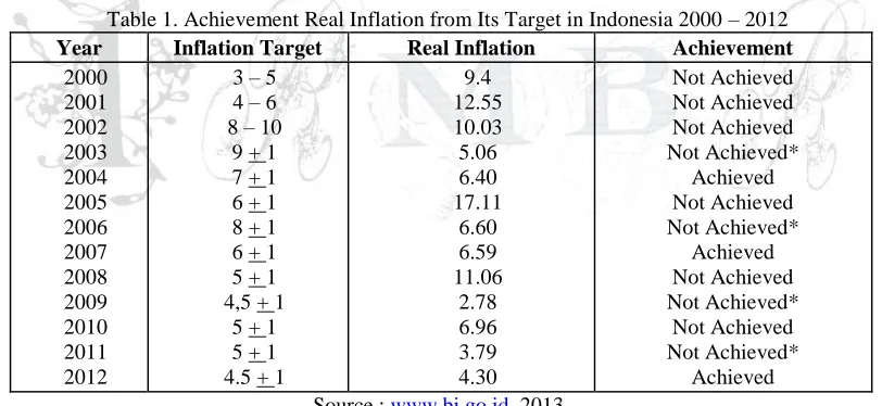
Empirical pre-conditions of ITF has not available been, so the implementation of ITF in Indonesia has not been satisfied either in decreasing inflation rate or in directing the actual inflation rate to its target (Table 1). The Table showed that real inflation rate was not in the range of its target. So it needed to evaluate monetary policy formulation by employing reaction function model opened economy instead of closed economy.

The aimed of the study were 1. to test and analyze real GDP lag, real GDP lead, real interest rate and real exchange rate affected output gap simultaneously and partially; 2. to test and analyze real GDP and SBI interest rate affected real money balance simultaneously and partially; 3. to test and analyze inflation lead, inflation lag, real GDP lag, real exchange rate lag, real exchange rate lag 2 affected inflation simultaneously and partially; 4. to test and analyze output gap and inflation gap affected SBI interest rate simultaneously and partially; 5. to test and analyze output gap, inflation gap and real exchange rate gap affected SBI interest rate simultaneously and partially; and then 6. to describe reaction function model of opened economy was better than model of closed economy.

Table 1. Achievement Real Inflation from Its Target in Indonesia 2000 – 2012

Year Inflation Target Real Inflation Achievement

2000 2001 2002 2003 2004 2005 2006 2007 2008 2009 2010 2011 2012

3 – 5 4 – 6 8 – 10

9 + 1 7 + 1 6 + 1 8 + 1 6 + 1 5 + 1 4,5 + 1

5 + 1 5 + 1 4.5 + 1

9.4 12.55 10.03 5.06 6.40 17.11

6.60 6.59 11.06

2.78 6.96 3.79 4.30

Not Achieved Not Achieved Not Achieved Not Achieved*

Achieved Not Achieved Not Achieved*

Not Achieved Not Achieved*

Achieved Source : www.bi.go.id, 2013.

The study is organized into five sections, first section was introduction, second section was theoretical framework, third section were conceptual framework, hypothesis and research method, fourth section were analyses and discussion, and five-th section were conclusion and recommandation.

Theoretical Framework

(3)

ISSN: 2306-9007 Adenan (2014) 213

I

nternational

R

eview of

M

anagement and

B

usiness

R

esearch

Vol. 3 Issue.1

R

M

B

R

Figure 1 displayed transmission model of Keynesian macro economics, comprised of fiscal side (Keynesian Cross) formed equilibrium on real sector (Investment Saving, IS) and monetary side formed equilibrium on monetary sector (Liquidity of Monetary Preference, LM), finally interaction of both constructs Aggregate Demand. On the other side Keynes assumed that Aggregate Supply passive but in the modern macro-economics, it might be derived from Phillip Curve where it figured a relation between change of wage rate and unemployment rate, then it was extended by identifying negative correlation between unemployment and real output, and finally it was relation between inflation rate and real output. Increasing inflation rate corresponded increasing real output, this pattern called as a short run aggregate supply. So in short run a general equilibrium was formed by aggregate demand and aggregate supply mechanism constructed AD-AS Model.

Figure 1. Theory of Short term Economics Fluctuation Sumber: Mankiw, 2003: 272

Regulation on monetary sector directed money supply and interest rate to support economics development. Monetary policy affects money supply and its demand as liquidity monetary preference theory. Monetary policy utilizes a regulation on real money balance and interest rate anchor to support macro-economic activities (Pohan, 2008: 11-12).

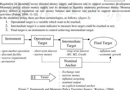
In the monetary policy there are three terminologies, as follows: (figure 2).

1.

Operational target is a variable which want to be reached;

2.

Intermediate target is a main indicator to measure how target could be reached or not;

3.

Final target is an instrument to control achieving intermediate target.

- open market operation - short term interest - long term interest - inflation rate - discount facility - narrow money - M1, M2, Credit - economic growth - reserve requirement

- persuasion

- Exchange rate

- narrow money

- inflation targeting

- nominal output

- no explicit nominal anchor

Figure 2. Framework and Monetary Policy Targeting Source : Warjiyo, (2004)

Keynesian Cross IS

Curve

Aggregate Demand IS-LM

Model

LM Curve Liquidity

Prefe-rence Theory

Explanation of short term Economics Fluctuation

AD-AS Model

Instrument

Final Target

Operational

Target

Intermediate

Target

Nominal

Anchor

Target

(4)

ISSN: 2306-9007 Adenan (2014) 214

I

nternational

R

eview of

M

anagement and

B

usiness

R

esearch

Vol. 3 Issue.1

R

M

B

R

Monetary policy based on rule, discretion, and combination of both. Authority utilizes a rule of monetary in a formula was announced in response of various situations. Then authority utilizes a discretion if it evaluates freely on various conditions and chosen any policy (Mankiw, 2003: 381). An empirical authority takes a combination of rule and discretion. Under discretion, sometime it motivated monetary authority acted inconsistent from former point (called of time inconsistent) and caused central bank was un-credible viewed by market agent. Monetary authority formerly had commitment to control inflation at given target rate, but the authority had often driven economics growth in short run. Monetary policy without clear objectives on price stability often looks monetary authority was un-credible.

The development monetary policy rule has become a model pioneered by Taylor (1993). Indonesia is one of emerging market countries that has advantages in adopting Taylor Rule. Practical ITF in many countries adopted and modified it as a rule with various anchors. Svensson (1999) argued that because of uncertain of some economic variables behavior employing interest rate as a single anchor was recommended. Bank Indonesia adopts a single anchor called SBI Rate in implementing ITF. SBI Rate was recommended by Mc Nelis (1999) and also Darsono et. al (2002) as a single instrument rule for managing inflation gap and output gap.

Conceptual Framework, Hypothesis and Research Method

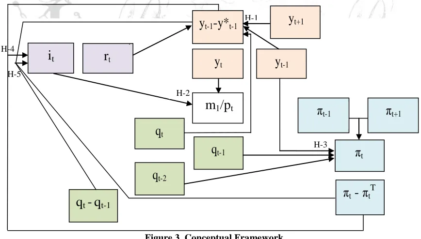
The Study formulated hypothesis as a conceptual framework categorized into two blocks as macro-economy block, symbolized as H-1, H-2 and H-3 and reaction function block, symbolized as H-4 and H-5, so a conceptual framework displayed on figure 3, as follows:

Figure 3. Conceptual Framework

Based on case formulation, literature of the study and former research, it would be proposed as Hypothesis, follows:

1. Real GDP lag, real GDP lead, real interest and real exchange rate simultaneously and partially

significant affected on output gap.

72

79

H-1

H-4

H-5

i

t

r

t

y

t-1

-y*

t-1

m

1

/p

t

π

t

y

t

y

t-1

y

t+1

π

t-1

q

t

-

q

t-1

q

t-1

π

t

- π

t T H-2

H-3

q

t-2

π

t+1

(5)

ISSN: 2306-9007 Adenan (2014) 215

I

nternational

R

eview of

M

anagement and

B

usiness

R

esearch

Vol. 3 Issue.1

R

M

B

R

2. Real GDP and SBI interest rate simultaneously and partially significant affected on real money balance.

3. Inflation rate lead, inflation lag, real GDP lag, real exchange rate lag and real exchange rate lag-2

simultaneously and partially significant affected on inflation rate.

4. Output gap and inflation gap simultaneously and partially significant affected on SBI interest rate.

5. Output gap, inflation gap and exchange rate gap simultaneously and partially significant affected

on SBI interest rate.

6. reaction function model of opened economy was better than closed economy one, was just

analized qualitatively.

The Study was explanatory to test and analyze reaction function model of monetary policy in the inflation targeting framework in Indonesia a period of 2000:1 – 2012:4 quarterly. It employed Statistical Package for Social Science (SPSS) and Solver Ad-in Microsoft Excel. The study was conducted into three steps, firstly formulated macro-economy model as Ball-Batini model, secondly set reaction function model, either closed or opened economy model, and thirdly evaluated social welfare loss function optimal.

1. Determined Macro-Economic Model

yt – yt*= -1yt-1 - 2Etyt+1 + 3(it - Et(πt-+1)) + 4qt + ε y

1t 4.1

mt / pt c

= β1yt - β2it + ε2t 4.2

πt = (1πt-1 + (1-1)πt+1) + 2yt-1 + 3qt-1 + 4qt-2 + ε5t 4.3

where:

et = (Etet+1 x it) / i f

t

qt = (et xpt c

/ pt cf

) εt = θu εt-1 + ηεt

2. Set Reaction Function Models:

a. A closed economy model

4.4 b. An opened economy model

4.5

3. Evaluated Social Welfare Loss Function (SWLF) Optimal:

Social Welfare Loss Function is a function which related how much social loss is affected by the policy adopted. The less SWLF the better, so the function looked for the less value of SWLF between both models. The study utilized conditional optimization of reaction function and employed Lagrange method which a new function which was calculated optimized reaction function plus Lagrange (λ) within its constraint function.

Minimized a Social Welfare Loss Function of closed economy Model:

Constraint functions comprised of:

1. yt – yt*= -1yt-1 - 2Etyt+1 + 3(it - Etπt-+1) + 4qt + εy1t 4.1

2. mt /ptc= β1yt - β2it + ε2t 4.2

3. πt = (1πt-1 + (1-1)πt+1) + 2yt-1 + 3qt-1 + 4qt-2 + ε3t 4.3



1



2



1 1



1

*



_



_





_



_



t t

T t t

t

r

y

i











1



2



1 1



3



1



1

*



_



_





_



_





_



t t t t

T t t

t

r

y

q

i











1



2



1 1



1

1  

*















T _t _t

t t

t

r

y

(6)

ISSN: 2306-9007 Adenan (2014) 216

I

nternational

R

eview of

M

anagement and

B

usiness

R

esearch

Vol. 3 Issue.1

R

M

B

R

4.4

4.5

so a new function as follows:

z = (rt + t-1 + 1 (t-1 - T) + 2 (yt-1 - yt-1*)) + λ ((-1yt-1 - 2Etyt+1 + 3(it - Etπt+1) + 4qt) + ( β1yt -

β2it) + ((1πt-1 + (1-1)πt+1) + 2yt-1 + 3qt-1 + 4qt-2))

Minimized a Social Welfare Loss Function of opened economy Model:

Constraint functions as same as above, so a new function as follows:

z = (rt + t-1 + 1 (t-1 - T) + 2 (yt-1 - yt-1*)+ 3(qt - qt-1)) + λ ((-1yt-1 - 2Etyt+1 + 3(it - Etπt+1) + 4qt) + ( β1yt -

β2it) + ((1πt-1 + (1-1)πt+1) + 2yt-1 + 3qt-1 + 4qt-2)) 4.5

The Study Result and Discussion

The study concluded that 1. real GDP lag, real GDP lead, real interest rate and real exchange rate simultaneously significant affected on output gap. Real GDP lag, real interest rate and real exchange rate partially significant affected on output gap, but real GDP lead did not; 2. real GDP and SBI interest rate simultaneously and partially significant affected on real money balance; 3. inflation lead, inflation lag, real GDP lag, real exchange rate lag and real exchange rate lag 2 simultaneously significant affected on inflation rate. Inflation lead and inflation lag restrictedly and real GDP lag partially significant affected on inflation, but real exchange rate lag and real exchange rate lag 2 did not; 4. output gap and inflation gap simultaneously significant affected on SBI interest rate. Inflation gap partially significant affected on SBI interest rate, but output gap did not; 5. output gap, inflation gap and exchange rate gap simultaneously significant affected on SBI interest rate. Inflation gap partially significant affected on SBI interest rate, but output gap and exchange rate gap did not. Reaction function model of opened economy was better than closed economy one. The models needed discretion more, shown that coefficient correlation for both model less than 0,18 and 0,22 each. All of independent variables in the models had been able to define dependent variable at 0,18% and 0,22%, while the rest other independent variables out of the model affected on dominantly.

As a part of global financial market, domestic monetary policy maker had to consider external factors, like exchange rate. ITF played role in decreasing inflation rate as implementing model, it should be adopted reaction function of opened economy model, because:

1. Indonesia as one of opened economy where fluctuation of exchange rate affected domestic economy,

as export-import in goods and services, payment offshore loan, private debt and its interest.

2. Money supply was not effectively as an intermediate target in monetary policy (Affandi, 2002), so it

needed effective monetary instruments such as nominal interest and exchange rate affected real output in short run in Indonesia (Siregar, 2008).

3. Character of inflation in Indonesia affected more by supply side and imported inflation, which could

not be responded just interest rate. So it needed coordination to solve supply side, whose government domain. ITF utilized SBI interest rate as a instrument needed to affect credit interest rate in interest rate policy. Like in the Fed, Bank Indonesia should be able to touch operational commercial bank as banker’s bank not just as the last lender resort.

4. IT needed freely floating exchange rate for developing countries, it seems hard to escape exchange rate fluctuation corresponding in global market condition. Although the study proved that exchange rate change did not affect inflation rate significant, but Bank Indonesia should looked at exchange rate change.



1



2



1 1



3



1



1

1  

*

 



















T _t _t _t _t

t t

t

r

y

q

(7)

ISSN: 2306-9007 Adenan (2014) 217

I

nternational

R

eview of

M

anagement and

B

usiness

R

esearch

Vol. 3 Issue.1

R

M

B

R

Factors were not easy to escape from exchange rate, as follows: (Ismail, 2006)

1. Perspective of Indonesia economy since 1997, exchange rate was famous variable for publics because the variable was often used for government and Bank Indonesia performance. Exchange rate change was also used as a prime base for economics agent to determine expected inflation and needed intervene to decrease the fluctuation.

2. Financial condition of firm, institution and government sectors were so sensitive to exchange rate

change.

3. Exchange rate affected un-comparable for profitable level between tradable and non tradable

goods, so it could be financial hard for certain sectors in economy.

Conclusion and Recommandations

Contribution on policy of the study “Reaction Function Model of Monetary Policy under Inflation Targeting Framework in Indonesia” was to enhance alternative reaction function model of monetary policy. It proved that reaction function model of opened economy was better than closed one. Even both models statisticly fulfilled clasical assumption, but they needed discretion more than rule.

Based on the study it recommended that: 1. Bank Indonesia should adopt reaction function model opened economy in formulating the future monetary policy; 2. Bank Indonesia should be powerful in directing inflation target and avoided crowding out by utilizing five pillars policy mix related with corresponded by government, consistent monetary policy to achieve inflation target, exchange rate policy to direct stability of Rupiah, and communication strategy to support policy effective; and 3. Bank Indonesia needs to revitalize monetary instrument like discount window to direct commercial bank to achieve inflation target.

References

Affandi, Yoga, 2002. The Optimal Monetary Policy Instruments:The Case of Indonesia, Buletin Ekonomi

Moneter dan Perbankan, Jakarta : BI Des:58

Alamsyah Halim, Judha Agung and D. Zukverdy. 2001. Towards implementation of Inflation Targeting In

Indonesia. Bulletin of Indonesian Economic Studies. ANU, Canberra.

Pohan, Aulia. 2008. Kerangka Kebijakan Moneter & Implementasinya di Indonesia. Jakarta: Raja Grafindo

Persada.

Batini, N and Haldane, AG 1999. Forward-Looking Rules for Monetary Policy. in Taylor John B, (ed). Monetary Policy Rules. Chicago: Univ. of Chicago and NBER.

Bernanke, Ben S. dan Reinhart, Vincent. 2004. Conduct Monetary Policy At Very Low Short-term Interest

Rates. American Economnic Review.

Ball, Laurence, 1998. Policy Rule For Open Economies. Reserve Bank of Australia.

Clarida, Richard, Jordi Gali dan Mark Getler. 1997. Monetary Policy Rules in Practice, Some International

Evidence. Center for Applied Economics.New York Ubiversity.

Darsono, Akhlis R Hutabarat, Rizki E Wimanda, Handayani dan Tri Yanuarti. 2002. Disain Monetary

Policy Rule Untuk Indonesia. Direktorat Riset Ekonomi Dan Kebijakan Moneter Bank Indonesia. Jakarta.

Fuhrer, Jeffrey C dan Madigan, Brian F 1997. Monetary Policy When Interest Rates Are Bounded At Zero.

Review of Economics and Statistics.

Gordon, De Brower dan James O’Ragan. 2000. Evaluating Simple Monetary Policy Rules For Australia.

Reserve Bank of Australia.

Ismail, Munawar, 2006. Inflasi Targeting Dan Tantangan Implementasinya Di Indonesia, Jurnal Ekonomi

dan Bisnis Indonesia, Volume 21, Nomor 2, Halaman 105-121, Yogyakarta.

Mc Callum, Bennet T. 1987. The Case For Rules in the Conduct of Monetary Policy. A Concrete Example.

(8)

ISSN: 2306-9007 Adenan (2014) 218

I

nternational

R

eview of

M

anagement and

B

usiness

R

esearch

Vol. 3 Issue.1

R

M

B

R

Mc Nelis, Paul D. 1999. Monetary Policy, the Role Learning and Inflation Targeting Implication For Bank

Indonesia. Direktorat Riset Ekonomi Dan Kebijakan Moneter BI. Jakarta.

Rotemberg, Julio dan Woodford, Michael. 1999. Interest Rate Rules Ib Estimated StickyPrice Models.

Dalam John B. Taylor, Monetary Policy Rules. Chicago University Press. Chicago

Rudebusch, Glan D dan Svensson, Lars E.O. 1998. Policy Rules For Inflation Targeting. Dalam John B.

Taylor, Monetary Policy Rules. Chicago University Press. Chicago.

Siregar, R. and S. Goo. 2008. Inflation Targeting Policy: The Experience of Indonesia and Thailand. Centre

for Applied Macroeconomic Analysis, The Australian National University, Working Paper 23/2008.

http://cama.anu.edu.auSvensson, Lars EO. 2006. Inflation Targeting. Princeton University.

Tanuwidjaja, Enrico and Keng meng Choy. 2005. Central Bank Credibility and Monetary Policy in Indonesia. Journal of Policy Modeling.

Taylor, John B. 1999. Discretion Versus Policy Rules In Practice. Carnegie Rochester Conference Series In

Public Policy.

Variables were symbolized, as follows:

yt : Real Gross Domestic Product

yt+1 : Real Gross Domestic Product Lead

yt-1 : Real Gross Domestic Product Lag

yt-1-y*t-1 : Output Gap

m1/pt : Real Money Balances

it : SBI or certificate of Bank Indonesia Interest Rate

rt : Real Interest Rate

πt : Inflation Rate

πt+1 : Inflation Rate Lead

πt-1 : Inflation Rate Lag

πt - πtT : Inflation Gap

qt : Real Exchange Rate

qt-1 : Real Exchange Rate Lag

qt-2 : Real Exchange Rate 2 periods Lag

qt -qt-1 : Real Exchange Rate Gap

APPENDIXES

Macro Economics Model:

Model Summaryd

Model

R

R Squar

e

Adjuste d R Square

Std. Error of the Estimate

Change Statistics Durbi

n-Watso

n R Square

Change F

Change df1 df2

Sig. F Change

1 .721a .520 .480 2.76854 .520 12.750 4 47 .000

2 .889b .790 .762 1.87114 .270 28.947 2 45 .000

3 .934c .873 .842 1.52742 .082 6.633 4 41 .000 1.025

a

Predictors: (Constant), Real Exchange Rate, natural Interest Rate, real PDB Lead, real PDB Lag

b_{Predictors: (Constant), Nominal Interest Rate of SBI, Real PDB}

c_{Predictors: (Constant), real PDB Lag, Inflation Rate Lag and Lead, Real Exchange Rate Lag and Lag-2}

(9)

ISSN: 2306-9007 Adenan (2014) 219

I

nternational

R

eview of

M

anagement and

B

usiness

R

esearch

Vol. 3 Issue.1

R

M

B

R

ANOVAd

Model

Sum of

Squares df Mean Square F Sig.

1 Regression 390.915 4 97.729 12.750 .000a

Residual 360.246 47 7.665

Total 751.161 51

2 Regression 593.609 6 98.935 28.258 .000b

Residual 157.552 45 3.501

Total 751.161 51

3 Regression 655.508 10 65.551 28.097 .000c

Residual 95.654 41 2.333

Total 751.161 51

a_{Predictors: (Constant), Real Exchange Rate, natural interest, Real PDB Lead, Real PDB Lag}

b

Predictors: (Constant), Nominal Interest Rate of SBI, Real PDB

c_{Predictors: (Constant), PDB Lag, Inflation Rate Lag and Lead, Real Exchange Rate Lag and Lag-2}

d_{Dependent Variable: Inflation rate}

Reaction Function Model Processed: a. Closed Economy Model

Model Summaryb

Mode

l R

R Square

Adjusted R Square

Change Statistics Durbin

-Watso

n R Square

Change F Chang

e df1 df2

Sig. F Change

1 _.465a

.216 .184 3.09689 .216 6.626 2 48 .003 .143

a_{Predictors: (Constant), Inflation Gap, Output Gap Lag}

b_{Dependent Variable: SBI Interest Rate}

ANOVAb

Model

Sum of

1 Regression 127.103 2 63.551 6.626 .003a

Residual 460.354 48 9.591

Total 587.456 50

a

Predictors: (Constant), Inflation Gap, Output Gap Lag

b. Opened Economy Model

Model Summaryb

Mode

l R

R Square

Adjusted R Square

Change Statistics Durbin

-Watso

n R Square

Change F Chang

e df1 df2

Sig. F Change

1 _.465a

.216 .166 3.12941 .216 4.329 3 47 .009 .146

a_{Predictors: (Constant),Inflation Gap, Output Gap Lag, Delta qt} b

(10)

ISSN: 2306-9007 Adenan (2014) 220

I

nternational

R

eview of

M

anagement and

B

usiness

R

esearch

Vol. 3 Issue.1

R

M

B

R

ANOVAb

Model

Sum of

1 Regression 127.174 3 42.391 4.329 .009a

Residual 460.282 47 9.793

Total 587.456 50

a_{Predictors: (Constant), Inflation Gap, Lag-1 output gap, Delta qt}

Optimization Social Welfare Loss Function (SWLF) a. Closed Economy Model:

Social welfare loss function was 8.77

Objective Function was to minimized value of reaction function

it = 8.772 + 0.505 (pt-1 - p T

) + 1.96E-005 (yt-1 - yt-1 *

)

Constraints Function were structural model, as follows:

yt - yt* =-0.960 yt-1 - 0.137 yt+1 - 0.424 (it - t+1) + 0.739 q1

mt/pt = - 0.784 yt + 1.145 it

t = t+1 t-1 + 0.208 yt-1 - 0.224 qt-1 - 0.087 qt-2

Zmin = 8.77

Optimum Minimum Maximum

Goods Market: -280739.76

Financial Market: 26730.42

Supply Aggregate: 51644.75

t-1 - T 0.00 -4.83 9.11

yt 340865.20 340865.20 671780.80

yt-1 256442.40 256442.40 671500.00

yt+1 286028.30 286028.30 671500.00

it 5.75 5.75 17.63

et x ptf / ptc 6266.67 6266.67 14663.87

t+1 2.78 2.78 17.11

t-1 1.17 1.17 17.11

qt-1 5447.84 5447.84 14663.87

qt-2 5447.84 5447.84 14663.87

qt - qt-1 0.00 -1864.68 2368.75

yt-1-yt-1* 0.00 -12602.65 17140.57

(11)

ISSN: 2306-9007 Adenan (2014) 221

I

nternational

R

eview of

M

anagement and

B

usiness

R

esearch

Vol. 3 Issue.1

R

M

B

R

b. Opened Economy Model:

Objective Function was to minimized value of reaction function

it t-1 - T) + 2.20E-005 (yt-1 - yt-1*) - 6.88E-005 (qt - qt-1)

Constraints Function were structural model, as follows:

yt - yt* =-0.960 yt-1 - 0.137 yt+1 - 0.424 (it - t+1) + 0.739 qt

mt/pt = - 0.784 yt + 1.145 it

t = 0 t+1 t-1 + 0.208 yt-1 - 0.224 qt-1 - 0.087 qt-2

Zmin = 8.62

Optimum Minimum Maximum

Goods Market: -280739.76

Financial Market: 26730.42

Supply Aggregate: 51644.75

t-1 - T 0.00 -4.83 9.11

yt 340865.20 340865.20 671780.80

yt-1 256442.40 256442.40 671500.00

yt+1 286028.30 286028.30 671500.00

it 5.75 5.75 17.63

et x ptf / ptc 6266.67 6266.67 14663.87

t+1 2.78 2.78 17.11

t-1 1.17 1.17 17.11

qt-1 5447.84 5447.84 14663.87

qt-2 5447.84 5447.84 14663.87

qt - qt-1 2368.75 -1864.68 2368.75

yt-1-yt-1* 0.00 -12602.65 17140.57

it- t+1 0.58 0.58 2.67