Learning Nondeterministic Classifiers

Learning Nondeterministic Classifiers

Juan Jos´e del Coz [email protected]

Jorge D´ıez [email protected]

Antonio Bahamonde [email protected]

Artificial Intelligence Center University of Oviedo at Gij´on Asturias, Spain

Editor: Lyle Ungar

Abstract

Nondeterministic classifiers are defined as those allowed to predict more than one class for some entries from an input space. Given that the true class should be included in predictions and the number of classes predicted should be as small as possible, these kind of classifiers can be con-sidered as Information Retrieval (IR) procedures. In this paper, we propose a family of IR loss functions to measure the performance of nondeterministic learners. After discussing such mea-sures, we derive an algorithm for learning optimal nondeterministic hypotheses. Given an entry from the input space, the algorithm requires the posterior probabilities to compute the subset of classes with the lowest expected loss. From a general point of view, nondeterministic classifiers provide an improvement in the proportion of predictions that include the true class compared to their deterministic counterparts; the price to be paid for this increase is usually a tiny proportion of predictions with more than one class. The paper includes an extensive experimental study using three deterministic learners to estimate posterior probabilities: a multiclass Support Vector Machine (SVM), a Logistic Regression, and a Na¨ıve Bayes. The data sets considered comprise both UCI multi-class learning tasks and microarray expressions of different kinds of cancer. We successfully compare nondeterministic classifiers with other alternative approaches. Additionally, we shall see how the quality of posterior probabilities (measured by the Brier score) determines the goodness of nondeterministic predictions.

Keywords: nondeterministic, multiclassification, reject option, multi-label classification,

poste-rior probabilities

1. Introduction

There are several learners that successfully solve classification tasks in which the number of classes is higher than two; see for instance Wu et al. (2004) and Lin et al. (2008). However, for each class

C most classification errors frequently occur between small subsets of classes that are somehow

similar to C, regardless of the approach used. This fact suggests that multiclass classifiers would increase in reliability if they were allowed to express their doubts whenever they were asked to classify some entries.

would be able to predict not just one single disease, but a set of options. These multiple predictions will be provided to domain experts when the classifier is not sure enough to give a unique class. Thus nondeterministic predictions may discard some options and allow domain experts to make practical decisions. Even when the nondeterministic classifier returns most of the available classes for the representation of an entry, we can read that the learned hypothesis is acknowledging its ignorance about how to deal with that entry.

It is evident that nondeterministic classifiers will include true classes in their predictions more frequently than deterministic hypotheses: they only have one possibility to be right. In this sense, nondeterministic predictions are backed by greater reliability. To be useful, however, nondetermin-istic classifiers should not only predict a set of classes containing the correct or true one, but their prediction sets should also be as small as possible. Notice that these requirements are common in algorithms designed for Information Retrieval. In this case, the queries are the entries to be classi-fied and the Recall and Precision are then applied to each prediction. Hence, the loss functions for

nondeterministic classifiers can be built as combinations of IR measures, as F_βfunctions are.

Starting from the distribution of posterior probabilities of classes, given one entry, we present an algorithm that computes the subset of classes with the lowest expected loss. In the experiments reported at the end of the paper, we employed three deterministic learners that provide posterior probabilities: Support Vector Machines (SVM), Logistic Regression (LR), and Na¨ıve Bayes (NB). We successfully compared the achievements of our nondeterministic classifiers with those obtained by other alternative approaches.

The paper is organized as follows. In the next section, we present an overview of related work on classifiers that return subsets of classes instead of a single class. The formal settings both for nondeterministic classifiers and their loss functions are presented in the third section. After that, in Section 4, we derive an algorithm to learn nondeterministic hypotheses. Then, we conclude the paper with a section in which we report an experimental study of their performance. In addition to the comparison mentioned above, we discuss the role played by the deterministic learner that provides posterior probabilities. We see that the quality of posterior probabilities determines the goodness of nondeterministic predictions. The data sets used are publicly available and, in addition to a group of data sets from the UCI Repository (Asuncion and Newman, 2007), they include a group of classification tasks of cancer patients from gene expressions captured by microarrays.

2. Related Work

Nondeterministic classifiers are somehow related to classifiers with reject option (Chow, 1970). In this approach, the entries that are likely to be misclassified are rejected, they are not classified and can be handled by more sophisticated procedures: a manual classification, for instance. The core as-sumption is that the cost of making a wrong decision is 1, while the cost of using the reject option is

given by some d, 0<d<1. In this context, provided that posterior probabilities are exactly known,

However, predictors of more than one class are not completely new. Given an ε∈[0,1], the so-called confidence machines make conformal predictions (Shafer and Vovk, 2008): they produce

a set of labels containing the true class with a probability greater than 1−ε.

To the best of our knowledge, the most directly related work to the approach presented in this paper is that of Zaffalon (2002) and Corani and Zaffalon (2008a,b). In these papers, the authors describe the Na¨ıve Credal Classifier, a set-valued classifier which is an extension of the Na¨ıve Bayes classifier to imprecise probabilities. The Na¨ıve Credal Classifier models prior ignorance about the distribution of classes by means of a set of prior densities (also called the prior credal set), which is turned into a set of posterior probabilities by element-wise application of Bayes’ rule. The classifier returns all the classes that are non-dominated by any other class according to the posterior credal set.

Another learning task that is related to this paper is multi-label classification. However, training instances in multi-label tasks can belong to more than one class, while nondeterministic training sets are the same as those of standard classification. In Tsoumakas and Katakis (2007), the au-thors provide an in-depth description of multi-label classification, enumerate several methods and compare their performance using Information Retrieval measures. Some applications have likewise arisen within the context of hierarchical organization of biological objects: predicting gene func-tions (Clare and King, 2003), or mapping biological entities into ontologies (Kriegel et al., 2004).

The formal setting presented in this paper was previously introduced in Alonso et al. (2008). There, we dealt with an interesting application of nondeterministic classifiers, in which classes (or ranks, in that context) are linearly ordered. The aim was to predict the rank (in an ordered scale) of carcasses of beef cattle. This value determines, on the one hand, the prices to be obtained by carcasses and, on the other, the genetic value of animals in order to select studs for the next generation. In this application, nondeterministic classifiers return an interval of ranks. Interval predictions are useful even when the intervals comprise more than one rank. For instance, it is possible to reject an animal as a stud for the next generation when a prediction interval is included in the lowest part of the scale. However, if we need a unique rank, we may decide to appeal to an

actual expert to resolve the ambiguity, an expensive classification procedure not always available in

practice.

The novelty of this paper is that now we deal with a standard classification setting; that is, the sets of classes are not ordered. This fact is very important as the search for the optimal prediction leads to a dramatic difference in complexity. Thus, if k is the number of classes, the search in the

ordinal case is just of order k2, while in the unordered case, at a first glance, the search is of order 2k.

However, the Theorem of Correctness of Algorithm 1 proves that this search can be accomplished in polynomial time.

Additionally, this paper reports an extensive experimental study. First, we test whether non-deterministic classifiers outperform Na¨ıve Credal Classifiers and other alternative approaches. We then investigate the role played by the ingredients of nondeterministic classifiers.

3. Formal Presentation and Notation

Let

X

Y

task given by a training set S={(x1,y1), . . . ,(xn,yn)}drawn from an unknown distribution Pr(X,Y)

Definition 1 A nondeterministic hypothesis is a function h from the input space to the set of

non-empty subsets of

Y

_Y

_Y

h :

X

Y

The aim of such a learning task is to find a nondeterministic hypothesis h from a space

H

optimizes the expected prediction performance (or risk) on samples S′independently and identically

distributed (i.i.d.) according to the distribution Pr(X,Y)

R∆(h) =

Z

∆(h(x),y)d(Pr(x,y)),

where∆(h(x),y)is a loss function that measures the penalty due to the prediction h(x)when the

true value is y.

In nondeterministic classification, we would like to favor those decisions of h that contain the true classes, and a smaller rather than a larger number of classes. In other words, we interpret

the output h(x) as an imprecise answer to a query about the right class of an entry x∈

X

nondeterministic classification can be seen as a kind of Information Retrieval task for each entry. Performance in Information Retrieval is compared using different measures in order to consider different perspectives. The most frequently used measures are Recall (proportion of all relevant documents that are found by a search) and Precision (proportion of retrieved documents that are relevant). The harmonic average of the two amounts is used to capture the goodness of a hypothesis

in a single measure. In the weighted case, the measure is called F_β. The idea is to measure a tradeoff

between Recall and Precision.

For further reference, let us recall the formal definitions of these Information Retrieval measures.

Thus, for a prediction of a nondeterministic hypothesis h(x)with x∈

X

Y

compute the following contingency matrix, where z∈

Y

y=z y6=z

z∈h(x) a b

z∈/h(x) c d

(1)

in which each entry (a,b,c,d) is the number of times that the corresponding combination of

mem-berships occurs. Notice that a can only be 1 or 0, depending on whether the class y is included in

the prediction h(x)or not; b is the number of classes different from y included in h(x); c=1−a;

and d is the number of classes different from y that are not included in h(x).

According to the matrix, Equation (1), if h is a nondeterministic hypothesis and(x,y)∈

X

Y

we thus have the following definitions.

Definition 2 The Recall in a query (i.e., an entry x) is defined as the proportion of relevant classes

(y) included in h(x):

R(h(x),y) = a

a+c=a=1y∈h(x).

Definition 3 The Precision is defined as the proportion of retrieved classes in h(x)that are relevant (y):

P(h(x),y) = a

a+b =

1y∈h(x)

h(x) Precision Recall F1 F2

[1,2,3] 0.33 1 0.50 0.71

[1,2] 0.50 1 0.67 0.83

[1] 1 1 1 1

[2,3,4] 0 0 0 0

Table 1: The Precision, Recall, F1, and F2for different predictions of a nondeterministic classifier

h for an entry x with class 1, (y=1)

In other words, given a hypothesis h, the Precision for an entry x, that is, P(h(x),y), is the probability

of finding the true class (y) of the entry (x) by randomly choosing one of the classes of h(x).

Finally, the tradeoff is formalized by

Definition 4 The F_βis defined, in general, by

F_β(h(x),y) =(1+β

2_)PR β2_P+R =

(1+β2_)a

(1+β2_)a+b+β2_c. (2)

Thus, for a nondeterministic classifier h and a pair(x,y),

F_β(h(x),y) =

(

1+β2

β2_+|h(x)| if y∈h(x)

0 otherwise. (3)

The most frequently used F-measure is F1. For ease of reference, let us state that

F1(h(x),y) =

2y∈h(x)

1+|h(x)|.

Notice that for deterministic classifiers, the accuracy is equal to Recall, Precision, and F_βgiven

that|h(x)|=1.

To illustrate the use of the F-measures of an entry, let us consider an example. If we assume that

the true class of an entry x is 1, (y=1), then, depending on the value of h(x), Table 1 reports the

Recall, Precision, F1, and F2. We observe that the reward attached to a prediction containing the

true class with another extra class ranges from 0.667 for F1 to 0.833 for F2; whereas the amounts

are lower when the prediction includes 2 extra classes.

Once we have the definition of F_βfor individual entries, it is straightforward to extend it to a

test set. Hence, when S′is a test set of size n, the average loss on it will be computed by

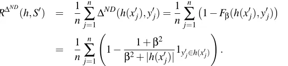
R∆ND(h,S′) = 1

n

n

∑

j=1

∆ND_(h(x′

j),y′j) =

1

n

n

∑

j=1

1−F_β(h(x′_j),y′_j)

(4)

= 1

n

n

∑

j=1

1− 1+β

2 β2_+|h(x′

j)|

1y′_j∈h(x′

j) !

.

The average Recall and Precision can be similarly defined. For ease of reference, let us remark

that the Recall is the proportion of times that h(x′)includes y′ and is thus a generalization of the

0 0.1 0.2 0.3 0.4 0.5 0.6 0.7 0.8 0.9 1.0

-4 -3 -2 -1 0 1 2 3 4

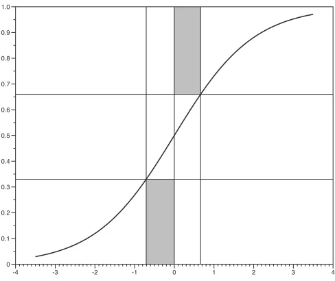
Figure 1: Conditional probabilities of class +1 given the discriminant value (horizontal axis) of

entries x∈

X

probability of over 1/3

3.1 Nondeterministic Classification in a Binary Task

To complete this section, let us show what nondeterministic classifiers look like in the simplest case, which will be further developed in the following sections. Let us assume that in a binary

classifica-tion task (the classes are codified by−1 and+1) we have a loss 1 for each false classification. On

the other hand, we are allowed to predict both classes, in which case the loss will be 1/3: the F1for

a classification of 2 classes containing the true one; see Table 1. The extension for dealing with F_β,

withβ6=1, is straightforward.

The optimum classifier will return only one class when it is sufficiently sure. In doubtful situa-tions, however, the nondeterministic classifier should opt for predicting the 2 classes. This will be

the case whenever the probability of error for both classes is higher than 1/3, since this is the loss

for predictions of two classes; see Figure 1. Therefore, if we have the conditional probabilities of classes given the entries, the optimum classifier will be given by

hND(x) =







{−1} i f η(x)<1/3

{−1,+1} i f 1/3≤η(x)<2/3

{+1} i f 2/3≤η(x),

(5)

where we are representing byη(x)the posterior probability:

η(x) =Pr(class= +1|x).

Notice that Equation (5) is equivalent to the generalized Bayes discriminant function described

in Bartlett and Wegkamp (2008) when the cost of using the reject option is calculated using the F1

Algorithm 1 The nondeterministic classifier nd•, an algorithm for computing the prediction with one or more classes for an entry x provided that the posterior probabilities of classes are given

Input:Cj: j=1, ..,k sorted by Pr(Cj|x)

Input:β: trade-off between Recall and Precision

Initialize i=0,∆0=1

repeat

i=i+1

∆i=1−1+β

2

β2_+i ∑i_j=1Pr(Cj|x) until((i==k)or(∆i−1≤∆i) if(∆i−1≤∆i)then

return{Cj: j=1, ..,i−1} else

return{Cj: j=1, ..,k} end if

4. Nondeterministic Classification Using Multiclass Posterior Probabilities

In the general multiclass setting presented at the beginning of Section 3, let x be an entry of the

input space

X

the entry, Pr(Cj|x). Additionally, we shall assume that the classes are ordered according to these

probabilities. In this context, we wish to define the

h(x) =Z⊂

Y

that minimizes the risk defined in Equation (1) when we use the nondeterministic loss given by F_β,

(Equations 2, 3, and 4). We shall prove that such an h(x)can be computed by Algorithm 1, which

does not need to search through all non-empty subsets of

Y

Theorem 1 (Correctness). If the conditional probabilities Pr(Cj|x)are known, Algorithm 1 returns

the nondeterministic prediction for h(x)that minimizes the risk given by the loss 1−F_β.

Proof To minimize the risk, Equation (1), it suffices to compute ∆x(Z) =

∑

y∈Y

∆ND_{(Z,y)Pr(y|x), (6)}

with Z⊂ {C1, . . . ,Ck}. Then, we only have to define

h(x) =argmin{∆x(Z): Z⊂ {C1, . . . ,Ck}}.

The proof has two parts. First, we shall see that if h(x)has r classes, then those are the r classes

with the highest probabilities; bearing in mind that classes are ordered, h(x) =Zr={Cj: j=1, ..,r}.

For this purpose, we need to see that any other subset of r classes will increase the loss due to Zr.

This is a consequence of the following.

The value of Equation (6) for Zris∆rin Algorithm 1. In fact, with the complementary

the other hand, with this sum of probabilities, the true class will be in h(x), and therefore the loss will be 1 minus the F_βof the prediction h(x) ={Cj: j=1, ..,r}:

∆x(Cj: j=1, ..,r) = 1− r

∑

j=1

Pr(Cj|x)

!

+ r

∑

j=1

Pr(Cj|x)

!

1−1+β

2 β2_+r

= 1−1+β

2 β2_+r

r

∑

j=1

Pr(Cj|x)

= ∆r.

Notice that for any other subset of r classes, we could achieve a similar expression simply by modifying the set of posterior probabilities of the last sum. Therefore, to minimize the value of Equation (6) with r classes, we need those with the highest probability.

In the second step, we only have to show that the index r returned by the Algorithm is the right one. We shall see that the search for the best r can be accomplished in linear time, as in the Algorithm. In fact, we shall establish that when the Algorithm reaches the number of classes with which the loss increases, adding further classes will only increase the loss. In symbols, we shall prove that

∆r≤∆r+1⇒∆r+1≤∆r+2.

To do so, we shall next express the exit condition of the loop∆r≤∆r+1when(r+1)≤k in a

different way. The following expressions are equivalent:

∆r≤∆r+1 (7)

1+β2 β2_+r

r

∑

j=1

Pr(Cj|x)≥

1+β2 β2_+r+1

r+1

∑

j=1

Pr(Cj|x)

(β2+r+1) r

∑

j=1

Pr(Cj|x)≥(β2+r)

r+1

∑

j=1

Pr(Cj|x)

r

∑

j=1

Pr(Cj|x)≥(β2+r)Pr(Cr+1|x).

Therefore, if∆r≤∆r+1and(r+1)≤k, then

Pr(Cr+1|x) +

r

∑

j=1

Pr(Cj|x)≥(β2+r)Pr(Cr+1|x) +Pr(Cr+1|x).

However, bearing in mind that the classes are ordered, we have that Pr(Cr+1|x)≥Pr(Cr+2|x),

and using Equation (7), we conclude that

r+1

∑

j=1

4.1 Corollaries

In order to draw some practical consequences, let us reword the previous Theorem. It states that the optimum classification for an input x is the set of r classes with the highest posterior probabilities, where r is the lowest integer that fulfills

r

∑

j=1

Pr(Cj|x)≥(β2+r)Pr(Cr+1|x), (8)

or the set of all classes when this condition is not fulfilled by any r. Expressed in this way, it is

straightforward to see that for two classes, withβ=1, Algorithm 1 coincides with the rule defined

in Equation (5).

Additionally, we would like to underscore that Equation (8) hinders the use of na¨ıve thresholds to compute nondeterministic predictions. Thus, a nondeterministic classifier that always predicts the top r classes for a constant value r is not a correct option. Equation (8) shows that r, at least, depends on the input x.

Moreover, we should not search for a threshold λto return, for all inputs, the first r classes

whose sum of probabilities is aboveλ:

r

∑

j=1

Pr(Cj|x)≥λ. (9)

Note that given aλvalue in[0,1], Equation (9) straightforwardly gives rise to a nondeterministic

classifier as follows. For each input x, if the set of classes is ordered according to their posterior probabilities, we define

h_λ(x) =

(

C1, . . . ,Cr: r

∑

j=1

Pr(Cj|x)≥λ & r−1

∑

j=1

Pr(Cj|x)<λ

)

. (10)

Again, the right-hand side of Equation (8) shows that the threshold (λ) would depend on the

number of classes predicted, the probability of the first class excluded from the prediction, and the

parameterβ: the trade-off between Precision and Recall. The idea behind Equation (8) is that, once

we have decided to include the top r classes, to add the(r+1)th _{class we should guarantee that}

Pr(Cr+1|x)is not much smaller than the sum of probabilities of the top r classes.

However, it may be argued that the inaccuracy of posterior probabilities would partially invali-date the preceding theoretical discussion. In fact, posterior probabilities are not known in practice: they are estimated by algorithms that frequently try to optimize the classification accuracy of a hypothesis that returns the class with the highest probability. In other words, probabilities are dis-criminant values instead of thorough descriptions of the distribution of classes in a learning task. Therefore, in the experiments reported at the end of the paper, we shall consider the classifiers defined by Equation (10) as a possible alternative method to the nondeterministic classifier of Algo-rithm 1.

5. Experimental Results

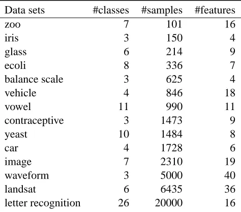
Data sets #classes #samples #features

zoo 7 101 16

iris 3 150 4

glass 6 214 9

ecoli 8 336 7

balance scale 3 625 4

vehicle 4 846 18

vowel 11 990 11

contraceptive 3 1473 9

yeast 10 1484 8

car 4 1728 6

image 7 2310 19

waveform 3 5000 40

landsat 6 6435 36

letter recognition 26 20000 16

Table 2: Description of the data sets downloaded from the UCI repository. The classes are not linearly separable

We have two goals here. On the one hand, we compare our approach with two alternative methods. The comparison will first be established with a state-of-the-art set-valued algorithm, the Na¨ıve Credal Classifier (NCC) (Zaffalon, 2002; Corani and Zaffalon, 2008a,b). This algorithm is an extension of the traditional Na¨ıve Bayes classifier towards imprecise probabilities and is designed to return robust set-valued (nondeterministic) classifications. We show that our method can improve the performance of NCC. We then contrast our method with an implementation of Equation (10); once again our proposals outperform this alternative way to learn nondeterministic classifiers.

On the other hand, we analyze the influence of a number of factors related to nondeterministic learners. We accordingly discuss how the scores of a nondeterministic learner are affected by the quality of posterior probabilities. We see that the performance of a nondeterministic classifier is highly correlated with the accuracy of its deterministic counterpart. The section ends with a study

of the meaning of the parameterβ.

5.1 Experimental Settings

We used three different methods for learning posterior probabilities in order to build nondeter-ministic classifiers. First, we employed the Na¨ıve Bayes (NB) used by NCC as its deternondeter-ministic counterpart (Corani and Zaffalon, 2008b). The second deterministic learner was a multiclass SVM; the implementation used was libsvm (Wu et al., 2004) with the linear kernel. Last, we employed the

logistic regression (LR) of Lin et al. (2008). It should be noted that we are not only using the

multi-class multi-classifiers learned by SVM or LR. Primarily, we apply the mechanisms that provide posterior probabilities from their outputs.

For each of these learners, we built ndd_{, where d stands for the name of the deterministic}

coun-terpart, nb, svm or lr. Recall that ndd is the implementation of Algorithm 1 that aims to optimize

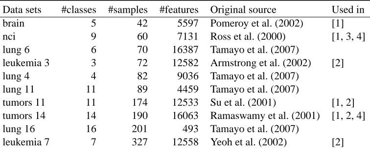
Data sets #classes #samples #features Original source Used in

brain 5 42 5597 Pomeroy et al. (2002) [1]

nci 9 60 7131 Ross et al. (2000) [1, 3, 4]

lung 6 6 70 16387 Tamayo et al. (2007)

leukemia 3 3 72 12582 Armstrong et al. (2002) [2]

lung 4 4 82 9036 Tamayo et al. (2007)

lung 11 11 89 4459 Tamayo et al. (2007)

tumors 11 11 174 12533 Su et al. (2001) [1, 2]

tumors 14 14 190 16063 Ramaswamy et al. (2001) [1, 2, 4]

lung 16 16 201 493 Tamayo et al. (2007)

leukemia 7 7 327 12558 Yeoh et al. (2002) [2]

Table 3: Description of cancer microarray data sets used in the experiments including the original sources and papers from which they are taken. For the sake of brevity, we have denoted the papers as follows: [1] Tibshirani and Hastie (2007), [2] Tan et al. (2005), [3] Staunton et al. (2001), [4] Yeung and Bumgarner (2003)

In the experiments that follow, we used two kinds of data sets. First, we considered data sets downloaded from the UCI repository (Asuncion and Newman, 2007), all of which have more ex-amples than attributes. We included all the data sets that fulfill the following rules: continuous or ordinal attribute values, no more than 40 attributes and no more than 20000 examples. The inten-tion was to consider small data sets that are not linearly separable. Addiinten-tionally, we excluded those learning tasks with missing values or in which every deterministic learner considered (NB, SVM,

LR) achieves a proportion of successful classifications of over 95%; otherwise nondeterministic

learners would be too similar to their deterministic counterpart. A description of the group of data sets considered can be found in Table 2.

We then evaluated the performance on learning tasks in which the aim was to classify cancer patients from gene expressions captured by microarrays. Unlike the first package of data sets, all the classes are now linearly separable given the dimensions of the input space and the number of entries. Table 3 shows the details of these data sets.

Every table of scores (Tables 4, 5, 6, 7, 8) is devoted to reporting the experimental results achieved in one of the kinds of data sets by one of the deterministic learners and by two nondeter-ministic algorithms that are to be compared. All the tables have a similar layout. First, they contain

the scores of the deterministic learner d: the F1(or accuracy or Recall), and the Brier score, a

mea-sure for the quality of posterior probabilities (Brier, 1950; Yeung et al., 2005), computed by means of

BS= 1

2n

n

∑

i=1 k

∑

j=1

([yi=Cj]−Pr(Cj|xi))2.

Then we report, for each nondeterministic learner, the F1, Precision, Recall, and the average number

of classes predicted (|h(x)|). All the scores were estimated by means of a 5-fold cross validation

repeated 2 times. We did not use the 10-fold procedure, since in certain data sets there are too few examples in some of the classes.

Following Demˇsar (2006), we used the Wilcoxon signed ranks test to compare the performance

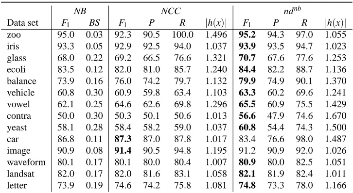
NB NCC ndnb

Data set F1 BS F1 P R |h(x)| F1 P R |h(x)|

zoo 95.0 0.03 92.3 90.5 100.0 1.496 95.2 94.3 97.0 1.055 iris 93.3 0.05 92.9 92.5 94.0 1.037 93.9 93.5 94.7 1.023 glass 68.0 0.22 69.2 66.5 76.6 1.321 70.7 67.6 77.6 1.253 ecoli 83.5 0.12 82.0 81.0 85.7 1.240 84.4 82.2 88.7 1.136 balance 73.9 0.16 76.0 74.2 79.7 1.132 79.9 74.9 90.1 1.370 vehicle 60.8 0.30 60.9 59.8 63.4 1.103 63.3 60.2 69.6 1.241 vowel 62.1 0.25 64.6 62.6 69.8 1.296 65.5 60.9 75.5 1.429 contra 50.0 0.30 50.3 50.1 50.6 1.013 56.6 47.9 74.6 1.670 yeast 58.1 0.28 58.4 58.2 59.0 1.037 60.8 54.4 74.3 1.500 car 86.8 0.11 87.3 87.0 87.8 1.017 83.4 76.6 98.0 1.487 image 90.9 0.08 91.4 90.5 94.8 1.195 91.2 90.9 92.0 1.026 waveform 80.1 0.17 80.1 80.0 80.4 1.007 80.9 80.0 82.5 1.051 landsat 82.0 0.17 82.0 81.6 83.1 1.058 82.1 81.9 82.4 1.011 letter 73.9 0.19 74.6 74.2 75.8 1.081 74.8 73.3 78.0 1.166

Table 4: Scores obtained by Na¨ıve Bayes, the Na¨ıve Credal Classifier and nondeterministic classi-fiers on UCI data sets using a 5-fold cross validation repeated 2 times. For ease of reading,

F1, Precision (P), and Recall (R) are expressed as percentages. The best nondeterministic

F1for each data set is boldfaced

explicitly stated, we use the expression statistically significant differences to mean that p<0.01.

Additionally, in order to provide a quick view of the order of magnitude of the scores, we have

boldfaced the best nondeterministic F1score for each data set.

To select the regularization parameter, C, for SVM and LR, we used a 2-fold cross validation

repeated 5 times performed on training sets. We searched within C∈[10−2, . . . ,102].

5.2 Nondeterministic Classifiers vs. Na¨ıve Credal Classifiers

In this subsection, we compare our nondeterministic learner with NCC (Corani and Zaffalon, 2008b), a state-of-the-art set-valued (nondeterministic) algorithm. In order to ensure a fair comparison, our approach uses the Na¨ıve Bayes (NB) employed by NCC as its deterministic counterpart. Table 4

reports the scores of NB, NCC and our algorithm ndnb.

The nondeterministic ndnbis significantly (remember that we are using Wilcoxon tests) better

than NCC both in Recall and F1. Moreover, ndnb wins in 12 out of 14 data sets in F1, and in 11

out of 14 in Recall. However, the scores in Precision and size of predictions are more balanced; the differences are not significant. In Precision, NCC wins in 5 cases, loses in 8, and there is 1 tie situation. The size scores are favorable to NCC in 8 out of 14 data sets.

To complete the comparison, we should discuss the results achieved on high dimensional data sets (Table 3). Nevertheless, we do not show the scores on each data set. The characteristics of these tasks are not appropriate for Na¨ıve Bayes (a large number of attributes with a small number of examples); therefore, the posterior probabilities of NB are poor (they are significantly worse than those achieved by SVM and LR) and this affects the performance of our nondeterministic algorithm and NCC. Our method tends to be almost deterministic, the average value for the size of predictions

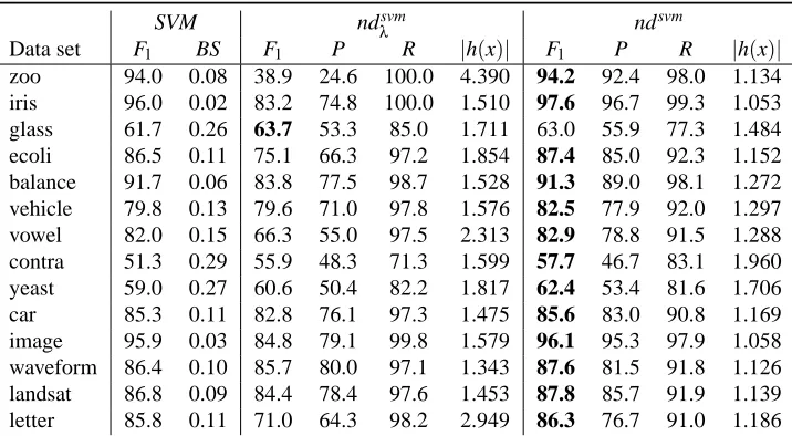
SVM nd_λsvm ndsvm

Data set F1 BS F1 P R |h(x)| F1 P R |h(x)|

zoo 94.0 0.08 38.9 24.6 100.0 4.390 94.2 92.4 98.0 1.134 iris 96.0 0.02 83.2 74.8 100.0 1.510 97.6 96.7 99.3 1.053 glass 61.7 0.26 63.7 53.3 85.0 1.711 63.0 55.9 77.3 1.484 ecoli 86.5 0.11 75.1 66.3 97.2 1.854 87.4 85.0 92.3 1.152 balance 91.7 0.06 83.8 77.5 98.7 1.528 91.3 89.0 98.1 1.272 vehicle 79.8 0.13 79.6 71.0 97.8 1.576 82.5 77.9 92.0 1.297 vowel 82.0 0.15 66.3 55.0 97.5 2.313 82.9 78.8 91.5 1.288 contra 51.3 0.29 55.9 48.3 71.3 1.599 57.7 46.7 83.1 1.960 yeast 59.0 0.27 60.6 50.4 82.2 1.817 62.4 53.4 81.6 1.706 car 85.3 0.11 82.8 76.1 97.3 1.475 85.6 83.0 90.8 1.169 image 95.9 0.03 84.8 79.1 99.8 1.579 96.1 95.3 97.9 1.058 waveform 86.4 0.10 85.7 80.0 97.1 1.343 87.6 81.5 91.8 1.126 landsat 86.8 0.09 84.4 78.4 97.6 1.453 87.8 85.7 91.9 1.139 letter 85.8 0.11 71.0 64.3 98.2 2.949 86.3 76.7 91.0 1.186

Table 5: Scores obtained by SVM learners on UCI data sets using a 5-fold cross validation repeated

2 times. For ease of reading, F1, Precision (P), and Recall (R) are expressed as percentages.

The best nondeterministic F1for each data set is boldfaced

LR ndlr

λ ndlr

Data set F1 BS F1 P R |h(x)| F1 P R |h(x)|

zoo 95.0 0.04 91.0 88.4 97.0 1.252 95.4 95.0 96.0 1.045 iris 96.7 0.05 74.4 61.7 100.0 1.767 94.4 92.2 99.0 1.137 glass 60.3 0.27 61.5 49.3 86.0 1.844 63.0 51.8 85.5 1.774 ecoli 87.5 0.11 76.9 68.3 96.1 1.668 87.0 84.4 92.1 1.173 balance 86.7 0.11 88.9 87.4 92.6 1.185 88.7 87.7 90.9 1.136 vehicle 77.0 0.16 74.8 64.9 95.3 1.674 79.2 74.1 89.7 1.342 vowel 57.9 0.30 54.1 41.5 83.5 2.226 57.8 48.6 79.7 1.908 contra 50.8 0.29 55.9 47.7 72.3 1.644 58.0 47.4 82.5 1.928 yeast 58.4 0.28 59.4 49.0 80.9 1.818 61.0 52.2 79.9 1.713 car 80.9 0.13 80.7 74.1 95.0 1.482 82.0 78.9 88.5 1.215 image 88.4 0.11 72.3 60.9 98.7 1.915 88.0 85.1 93.8 1.196 waveform 86.5 0.10 81.8 72.8 99.6 1.536 87.4 82.9 96.4 1.272 landsat 77.7 0.18 68.6 58.1 93.8 1.940 76.6 71.7 86.9 1.387 letter 71.8 0.24 49.3 36.5 90.7 3.253 70.3 64.9 82.5 1.556

Table 6: Scores obtained by LR learners on UCI data sets using a 5-fold cross validation repeated 2

times. For ease of reading, F1, Precision (P), and Recall (R) are expressed as percentages.

The best nondeterministic F1for each data set is boldfaced

the scores of NCC on these data sets are inadmissible; their classifiers predict almost all classes for

every example, their average values are: F1=25.73, P=15.39, R=100, and|h(x)|=8.58.

SVM nd_λsvm ndsvm

Data set F1 BS F1 P R |h(x)| F1 P R |h(x)|

brain 81.8 0.15 59.2 44.9 97.5 2.504 82.9 78.0 93.8 1.401 nci 48.3 0.35 42.9 33.2 68.3 2.492 47.7 41.4 65.0 2.167 lung 6 72.1 0.21 65.7 57.9 85.7 1.907 73.0 70.4 78.6 1.221 leukemia 3 94.5 0.04 75.1 64.5 100.0 1.862 95.7 94.9 97.3 1.049 lung 4 87.1 0.11 73.9 63.0 96.9 1.743 87.3 85.3 91.4 1.122 lung 11 58.4 0.31 49.3 36.5 84.2 2.656 60.4 53.8 78.0 1.903 tumors 11 89.6 0.13 30.6 19.1 99.7 6.135 88.9 87.1 92.8 1.199 tumors 14 70.0 0.26 45.0 35.3 95.0 4.550 66.5 60.2 84.7 2.021 lung 16 84.8 0.17 25.0 14.5 100.0 7.440 87.3 83.1 95.8 1.266 leukemia 7 92.0 0.07 70.1 59.9 99.4 2.216 92.1 90.6 95.1 1.090

Table 7: Scores obtained by SVM learners on cancer microarray data sets using a 5-fold cross

vali-dation repeated 2 times. For ease of reading, F1, Precision (P), and Recall (R) are expressed

as percentages. The best nondeterministic F1for each data set is boldfaced

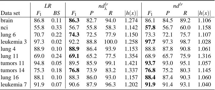
LR ndlr_λ ndlr

Data set F1 BS F1 P R |h(x)| F1 P R |h(x)|

brain 86.8 0.11 86.3 82.7 94.0 1.274 86.1 84.5 89.2 1.106 nci 55.8 0.33 56.7 55.8 58.3 1.142 57.8 56.7 60.0 1.158 lung 6 70.7 0.22 74.3 72.5 77.9 1.150 73.3 72.1 75.7 1.107 leukemia 3 97.3 0.02 92.2 88.8 100.0 1.258 97.7 97.3 98.7 1.028 lung 4 88.9 0.10 88.9 86.4 93.9 1.153 88.8 87.8 90.8 1.061 lung 11 69.0 0.24 69.1 65.2 77.5 1.354 68.9 65.7 75.9 1.316 tumors 11 94.8 0.05 89.5 85.9 99.1 1.421 93.7 93.0 95.1 1.057 tumors 14 75.3 0.18 76.8 73.9 83.2 1.337 76.8 75.2 80.3 1.145 lung 16 88.1 0.10 88.3 86.0 93.0 1.157 88.4 87.4 90.3 1.060 leukemia 7 91.9 0.07 90.6 87.9 96.3 1.202 91.9 91.4 93.1 1.040

Table 8: Scores obtained by LR learners on cancer microarray data sets using a 5-fold cross

valida-tion repeated 2 times. For ease of reading, F1, Precision (P), and Recall (R) are expressed

as percentages. The best nondeterministic F1for each data set is boldfaced

to increase. However the correlation between the accuracy of NB and|h(x)|of NCC is 0.24. In the

case of ndnb, this correlation is−0.75: negative and quite high.

5.3 Comparing nd with Another Alternative Method

In accordance with the discussion in Section 4.1, we shall now compare the nondeterministic clas-sifiers learned by Algorithm 1 with the alternative classifier defined in Equation (10) that uses a

thresholdλ for the sum of posterior probabilities. The comparison will be established with

pos-terior probabilities provided by SVM and LR given that both outperform the accuracy achieved by

Na¨ıve Bayes classifiers in the data sets used in these experiments. Theλnondeterministic classifiers

will be denoted by nd_λd, where d stands for the deterministic counterpart.

To select the parameterλ, we use a grid search employing a 2-fold cross validation repeated 5

times, aiming to optimize F1. The searching space depends on the learning task S. If the proportion

λ∈[a0,a1, . . . ,a5]; six options distribute from a to 0.99. In symbols, a0=a,a5=0.99, and ai+1−

ai=0.99₅−a.

In UCI data sets, Tables 5 and 6, ndsvm and ndlr win the corresponding nd_λ in 13 out of 14

data sets in F1 and Precision. In Recall we have the opposite situation;λclassifiers win in 13 out

of 14 cases. Moreover, λ classifiers always predict more classes than ndsvm and ndlr. In other

words,λclassifiers predict more classes than necessary. All differences are significant. Thus, our

nd classifiers are better than those computed with theλparameter.

In cancer microarray data, Tables 7 and 8, ndsvm always wins in F1, Precision, and average

|h(x)|; while ndsvm always loses in Recall. All differences are again significant. However, when

posterior probabilities are provided by LR, the differences are not significant in F1, although ndlr

has 5 wins, 1 tie and 4 losses; in Precision and average size of predictions the differences are

significant in favor of ndlr. Furthermore, as usual, the Recall is significantly higher forλclassifiers.

The conclusion is thatλclassifiers seem to need more classes in their predictions than nd

clas-sifiers. In fact, Equation (9) only considers the Recall. In practice, this means more Recall, but

less Precision and F1. Therefore, to optimize the F1 measure, in an experimental environment,

Equation (8) is more adequate than Equation (9), as we have conjectured theoretically in Section 4.1.

5.4 The Importance of Posterior Probabilities

The objective of this subsection is to experimentally investigate the degree of dependency between nondeterministic scores and the accuracy of posterior probabilities. In this study we again employ

SVM and LR with the collection of data sets detailed in Tables 2 and 3.

Let us first consider the set of UCI data sets. Comparing the results in Tables 5 and 6, it can

be seen that the scores of ndlr_{are significantly worse than those of nd}svm _{in F}

1, Precision, Recall

(p<0.03), and in average size of predictions. The general message is that ndlrinclude unnecessary

classes in their predictions. The base posterior probabilities seem to be the cause of this behavior: the Brier score of LR is significantly worse than that of SVM.

On the other hand, the scores obtained with cancer microarray data sets are shown in Tables 7 and 8. The characteristics of UCI and microarray data sets are quite different, and this affects the performance of classifiers. The main difference is that LR now has a significantly better Brier

score than SVM. Moreover, the ndlr _{algorithm achieves better results than nd}svm_{. The differences}

are significant in F1, Precision, Recall (p<0.02), and average|h(x)|. Yet again, inferior posterior

probabilities seem to be responsible for the inclusion of unnecessary classes in nondeterministic predictions.

In the preceding discussion of the scores achieved by nondeterministic learners, we found sig-nificant differences when the Brier scores of the deterministic counterparts presented sigsig-nificant differences. In fact, the scores of a learner built with Algorithm 1 depend on the quality of the pos-terior probabilities supplied by the corresponding deterministic learner. It seems plausible to draw the conclusion that the better the posterior probabilities, the better the nondeterministic scores. In

order to quantify this statement, we compared deterministic Brier scores with nondeterministic F1,

Recall, and Precision values; see Figure 2. We separated the scores achieved by UCI and cancer

data sets and included the scores of ndnb in UCI data sets. Similar results would be achieved if we

nd-svm Fit of nd-svm nd-lr Fit of nd-lr nd-nb

Fit of nd-nb

Correlation: -0.9914 Correlation: -0.9941 Correlation: -0.9802 F1 45 50 55 60 65 70 75 80 85 90 95 100 Brier score

0 0.05 0.10 0.15 0.20 0.25 0.30

F1 vs Brier score (UCI)

nd-svm Fit of nd-svm nd-lr Fit of nd-lr

Correlation: -0.9754 Correlation: -0.9984 F1 45 50 55 60 65 70 75 80 85 90 95 100 Brier score

0 0.05 0.10 0.15 0.20 0.25 0.30 0.35 0.40

F1 vs Brier score (Cancer)

nd-svm Fit of nd-svm nd-lr Fit of nd-lr nd-nb Fit of nd-nb Correlation: -0.9424 Correlation: -0.9487 Correlation: -0.9409 Recall 55 60 65 70 75 80 85 90 95 100 Brier score

0 0.05 0.10 0.15 0.20 0.25 0.30

Recall vs Brier score (UCI)

nd-svm Fit of nd-svm nd-lr Fit of nd-lr

Correlation: -0.8938 Correlation: -0.9941 Recall 55 60 65 70 75 80 85 90 95 100 Brier score

0 0.05 0.10 0.15 0.20 0.25 0.30 0.35 0.40

Recall vs Brier score (Cancer)

nd-svm Fit of nd-svm nd-lr Fit of nd-lr nd-nb Fit of nd-nb

Correlation: -0.9849 Correlation: -0.9889 Correlation: -0.9518 Precision 35 40 45 50 55 60 65 70 75 80 85 90 95 100 Brier score

0 0.05 0.10 0.15 0.20 0.25 0.30

Precision vs Brier score (UCI)

nd-svm Fit of nd-svm nd-lr

Fit of nd-lr Correlation: -0.9826

Correlation: -0.9960 Precision 35 40 45 50 55 60 65 70 75 80 85 90 95 100 Brier score

0 0.05 0.10 0.15 0.20 0.25 0.30 0.35 0.40

Precision vs Brier score (Cancer)

Figure 2: Correlation between Brier scores and F1, Recall, and Precision. The left column shows

the results with UCI data sets, while the right column uses cancer data sets. Similar results would be achieved if we compared nondeterministic scores with deterministic accuracy

We observed that the correlations between the Brier scores of deterministic learners and

non-deterministic scores (F1, Recall, and Precision) are very high: their absolute values are in all cases

greater than 0.89. Therefore, in order to choose a nondeterministic approach in a practical

F1 F2 Precision Recall 0.20 0.25 0.30 0.35 0.40 0.45 0.50 0.55 0.60 0.65 0.70 0.75 0.80 0.85 0.90 0.95 1.00 Beta

0 0.5 1.0 1.5 2.0 2.5 3.0 3.5 4.0

ndsvm _(yeast)

F1 F2 Precision Recall 0.20 0.25 0.30 0.35 0.40 0.45 0.50 0.55 0.60 0.65 0.70 0.75 0.80 0.85 0.90 0.95 1.00 Beta

0 0.5 1.0 1.5 2.0 2.5 3.0 3.5 4.0

ndsvm _(vowel)

F1 F2 Precision Recall 0.20 0.25 0.30 0.35 0.40 0.45 0.50 0.55 0.60 0.65 0.70 0.75 0.80 0.85 0.90 0.95 1.00 Beta

0 0.5 1.0 1.5 2.0 2.5 3.0 3.5 4.0

ndlr (yeast)

F1 F2 Precision Recall 0.20 0.25 0.30 0.35 0.40 0.45 0.50 0.55 0.60 0.65 0.70 0.75 0.80 0.85 0.90 0.95 1.00 Beta

0 0.5 1.0 1.5 2.0 2.5 3.0 3.5 4.0

ndlr (vowel)

F1 F2 Precision Recall 0.20 0.25 0.30 0.35 0.40 0.45 0.50 0.55 0.60 0.65 0.70 0.75 0.80 0.85 0.90 0.95 1.00 Beta

0 0.5 1.0 1.5 2.0 2.5 3.0 3.5 4.0

ndnb (yeast)

F1 F2 Precision Recall 0.20 0.25 0.30 0.35 0.40 0.45 0.50 0.55 0.60 0.65 0.70 0.75 0.80 0.85 0.90 0.95 1.00 Beta

0 0.5 1.0 1.5 2.0 2.5 3.0 3.5 4.0

ndnb (vowel)

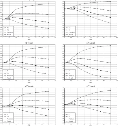
Figure 3: Evolution of F1, F2, Precision and Recall on two UCI data sets (yeast and vowel) for

differentβvalues and for the nondeterministic learners generated by SVM, LR, and NB

5.5 The Meaning ofβ

In this subsection, we analyze from the point of view of the user the role played by the parameterβin

Algorithm 1. Its theoretical aim is to control the size of predictions: as theβvalue increases, the size

of predictions will become bigger and therefore the Recall scores will be higher; see Equation (8).

The problem is that it is not always of interest to increase Recall values, since that would worsen F1

scores: adding more classes in predictions increases incorrect answers.

In Figure 3 we show the evolution of F1, F2, Precision and Recall on two UCI data sets (yeast

NB. Quite similar graphs could have been generated for the other data sets used in the experiments

reported in this section.

Initially,β=0 makes the nondeterministic classifiers deterministic. Therefore, the scores

rep-resented in the left-hand side of all the graphs in Figure 3 are all the same: the accuracy of the

de-terministic classifier. Asβvalues become higher, the Recall increases and the Precision decreases.

The main goal of the learning method proposed here is to look for a tradeoff of these measures that

is determined byβ, a user-modifiable parameter.

In practice, the value ofβthat the classifier must aim to optimize should be fixed by an expert

in the field of application in which the classifier is going to be employed. The kind of decisions that one would like to take from nondeterministic classifications must be considered.

It can be observed in the graphs in Figure 3 that the best scores in F1 are not always achieved

forβ=1. With small values ofβ, F1 increases. However, when some point near 1 is exceeded,

the F1score of the nondeterministic learner typically falls below the accuracy of the corresponding

deterministic learner. Nonetheless, optimal values are frequently reached around the nominal value:

β=1 (or 2 respectively). Slight improvements can be achieved in F1(in general Fβ) if we use a grid

search forβvalues to be used in Algorithm 1.

6. Conclusions

We have studied classifiers that are allowed to predict more than one class for entries from an input space: nondeterministic or set-valued classifiers. Using a clear analogy with Information Retrieval,

we have proposed a family of loss functions based on F_βmeasures. After discussing such measures,

we derived an algorithm to learn optimal nondeterministic hypothesis. Given an entry from the input space, the algorithm requires the posterior probabilities to compute the subset of classes with the lowest expected loss.

The paper includes a set of experiments carried out on two collections of data sets. The first one was downloaded from the UCI repository, the classes of which are not linearly separable. The sec-ond group is formed by data sets whose input spaces represent microarray expressions of different kinds of cancer, the classes of which are separable.

Using these benchmarks, we first compared nondeterministic learners obtained from a Na¨ıve Bayes with those learned by a state-of-the-art set-valued (nondeterministic) algorithm, the Na¨ıve Credal Classifier (NCC) (Zaffalon, 2002; Corani and Zaffalon, 2008a,b), an extension of the tradi-tional Na¨ıve Bayes classifier designed to return robust set-valued classifications. We showed that, using the loss measures defined in this paper, our method can improve the performance of NCC. Additionally, an important advantage of our nondeterministic classifiers over NCC is that we can control the degree of nondeterministic behavior. We can regulate the number of classes predicted by

fixing the F_βto be optimized: asβis higher (the weight of Recall is increased in the harmonic

aver-age F_β), the size of our predictions grows (see Section 5.5). However the nondeterministic behavior

of NCC is quite difficult to predict.

In addition to Na¨ıve Bayes, we used a multiclass SVM and a Logistic Regression. With the posterior probabilities provided by these deterministic learners, we built another alternative method to predict more than one class: the set of classes which the highest posterior probabilities summing

more than a thresholdλ. We also found that the classifiers built with our algorithm outperform this

On the other hand, in the experiments reported in this paper, we studied the role of the determin-istic learners that explicitly provide posterior probabilities. We found that the better the posterior probabilities, the better the nondeterministic classifiers. In fact we obtained very high correlations

between the Brier scores of deterministic probabilities and the F1, Precision and Recall values of

their nondeterministic counterparts.

Acknowledgments

The research reported here is supported in part under grants TIN2005-08288 from the MEC (Minis-terio de Educaci´on y Ciencia, Spain) and TIN2008-06247 from the MICINN (Minis(Minis-terio de Ciencia e Innovaci´on, Spain). We would also like to acknowledge all those people who generously shared the data sets and software used in this paper, and the anonymous reviewers, whose comments sig-nificantly improved it.

References

J. Alonso, J. J. del Coz, J. D´ıez, O. Luaces, and A. Bahamonde. Learning to predict one or more ranks in ordinal regression tasks. Proceedings of the European Conference on Machine Learning

and Principles and Practice of Knowledge Discovery in Databases (ECML PKDD’08), LNAI

5211, pages 39–54. Springer, 2008.

S.A. Armstrong, J.E. Staunton, L.B. Silverman, R. Pieters, M.L. den Boer, M.D. Minden, S.E. Sallan, E.S. Lander, T.R. Golub, and S.J. Korsmeyer. MLL translocations specify a distinct gene expression profile that distinguishes a unique leukemia. Nature Genetics, 30(1):41–47, 2002.

A. Asuncion and D.J. Newman. UCI machine learning repository. School of Information and

Computer Sciences. University of California, Irvine, California, USA, 2007.

P.L. Bartlett and M.H. Wegkamp. Classification with a reject option using a hinge loss. Journal of

Machine Learning Research, 9:1823–1840, 2008.

G.W. Brier. Verification of forecasts expressed in terms of probability. Monthly Weather Rev, 78: 1–3, 1950.

C. Chow. On optimum recognition error and reject tradeoff. IEEE Transactions on Information

Theory, 16(1):41–46, 1970.

A. Clare and R.D. King. Predicting gene function in Saccharomyces cerevisiae. Bioinformatics, 19 (2):42–49, 2003.

G. Corani and M. Zaffalon. Learning reliable classifiers from small or incomplete data sets: The Naive Credal Classifier 2. Journal of Machine Learning Research, 9:581–621, 2008a.

G. Corani and M. Zaffalon. JNCC2: The java implementation of Naive Credal Classifier 2. Journal

of Machine Learning Research (Machine Learning Open Source Software), 9:2695–2698, 2008b.

J. Demˇsar. Statistical comparisons of classifiers over multiple data sets. Journal of Machine

H.P. Kriegel, P. Kroger, A. Pryakhin, and M. Schubert. Using support vector machines for classi-fying large sets of multi-represented objects. Proc. 4th SIAM Int. Conf. on Data Mining, pages 102–114, 2004.

C-J. Lin, R. C. Weng, and S. S. Keerthi. Trust region newton method for logistic regression. Journal

of Machine Learning Research, 9(Apr):627–650, 2008.

S. L. Pomeroy, P. Tamayo, M. Gaasenbeek, L. M. Sturla, M. Angelo, M. E. McLaughlin, J. Y. H. Kim, L. C. Goumnerova, P. M. Black, C. Lau, J. C. Allen, D. Zagzag, J. M. Olson, T. Cur-ran, C. Wetmore, J. A. Biegel, T. Poggio, S. Mukherjee, R. Rifkin, A. Califano, G. Stolovitzky, D. N. Louis, J. P. Mesirov, E. S. Lander, and T. R. Golub. Prediction of central nervous system embryonal tumour outcome based on gene expression. Nature, 415(6870):436–442, 2002.

S. Ramaswamy, P. Tamayo, R. Rifkin, S. Mukherjee, C.H. Yeang, M. Angelo, C. Ladd, M. Reich, E. Latulippe, J.P. Mesirov, et al. Multiclass cancer diagnosis using tumor gene expression signa-tures. Proceedings of the National Academy of Sciences (PNAS), 98(26):15149–15154, 2001.

D.T. Ross, U. Scherf, M.B. Eisen, C.M. Perou, C. Rees, P. Spellman, V. Iyer, S.S. Jeffrey, M. Van de Rijn, M. Waltham, et al. Systematic variation in gene expression patterns in human cancer cell lines. Nature Genetics, 24(3):227–234, 2000.

G. Shafer and V. Vovk. A tutorial on conformal prediction. Journal of Machine Learning Research, 9:371–421, 2008.

J.E. Staunton, D.K. Slonim, H.A. Coller, P. Tamayo, M.J. Angelo, J. Park, U. Scherf, J.K. Lee, W.O. Reinhold, J.N. Weinstein, et al. Chemosensitivity prediction by transcriptional profiling.

Proceedings of the National Academy of Sciences (PNAS), 98(19):10787–10792, 2001.

A.I. Su, J.B. Welsh, L.M. Sapinoso, S.G. Kern, P. Dimitrov, H. Lapp, P.G. Schultz, S.M. Powell, C.A. Moskaluk, H.F. Frierson, and G. M. Hampton. Molecular classification of human carcino-mas by use of gene expression signatures. Cancer Research, 61(20):7388–7393, 2001.

P. Tamayo, D. Scanfeld, B.L. Ebert, M.A. Gillette, C.W.M. Roberts, and J.P. Mesirov. Metagene projection for cross-platform, cross-species characterization of global transcriptional states.

Pro-ceedings of the National Academy of Sciences (PNAS), 104(14):5959–5964, 2007.

A.C. Tan, D.Q. Naiman, L. Xu, R.L. Winslow, and D. Geman. Simple decision rules for classifying human cancers from gene expression profiles. Bioinformatics, 21(20):3896–3904, 2005.

R. Tibshirani and T. Hastie. Margin trees for high-dimensional classification. Journal of Machine

Learning Research, 8:637–652, 2007.

G. Tsoumakas and I. Katakis. Multi-label classification: An overview. International Journal of

Data Warehousing and Mining, 3(3):1–13, 2007.

E.J. Yeoh, M.E. Ross, S.A. Shurtleff, W.K. Williams, D. Patel, R. Mahfouz, F.G. Behm, S.C. Rai-mondi, M.V. Relling, A. Patel, C. Cheng, D. Campana, D. Wilkins, X. Zhou, J. Li, H. Liu, C.-H. Pui, W. E. Evans, C. Naeve, L. Wong, and J. R. Downing. Classification, subtype discovery, and prediction of outcome in pediatric acute lymphoblastic leukemia by gene expression profiling.

Cancer Cell, 1(2):133–143, 2002.

K.Y. Yeung and R.E. Bumgarner. Multiclass classification of microarray data with repeated mea-surements: application to cancer. Genome Biology, 4(12):R83, 2003.

K.Y. Yeung, R.E. Bumgarner, and A.E. Raftery. Bayesian model averaging: development of an improved multiclass, gene selection and classification tool for microarray data. Bioinformatics, 21(10):2394–2402, 2005.