R E S E A R C H
Open Access
A neural network-based framework for
financial model calibration
Shuaiqiang Liu
1*, Anastasia Borovykh
2, Lech A. Grzelak
1and Cornelis W. Oosterlee
1,2*Correspondence:[email protected]
1Applied Mathematics (DIAM), Delft University of Technology, Delft, The Netherlands
Full list of author information is available at the end of the article
Abstract
A data-driven approach called CaNN (Calibration Neural Network) is proposed to calibrate financial asset price models using an Artificial Neural Network (ANN). Determining optimal values of the model parameters is formulated as training hidden neurons within a machine learning framework, based on available financial option prices. The framework consists of two parts: a forward pass in which we train the weights of the ANN off-line, valuing options under many different asset model parameter settings; and a backward pass, in which we evaluate the trained
ANN-solver on-line, aiming to find the weights of the neurons in the input layer. The rapid on-line learning of implied volatility by ANNs, in combination with the use of an adapted parallel global optimization method, tackles the computation bottleneck and provides a fast and reliable technique for calibrating model parameters while avoiding, as much as possible, getting stuck in local minima. Numerical experiments confirm that this machine-learning framework can be employed to calibrate
parameters of high-dimensional stochastic volatility models efficiently and accurately.
Keywords: Computational finance; Machine learning; Artificial neural networks; Asset pricing model; Model calibration; Global optimization; Parallel computing
1 Introduction
Model calibration can be formulated as an inverse problem, where, based on observed output results, the input parameters need to be inferred. Previous work on solving inverse
problems includes research on adjoint optimization methods [2,8], Bayesian methods [4,
22], and sparsity regularization [7].
In a financial context, e.g., in the pricing and risk management of financial derivative contracts, asset model calibration means recovering the model parameters of the under-lying stochastic differential equations (SDEs) from observed market data. In other words, in the case of stocks and financial options, the calibration aims to determine the stock model parameters such that heavily traded, liquid option prices can be recovered by the mathematical model. The calibrated asset models are subsequently used to either deter-mine a suitable price for over-the-counter (OTC) exotic financial derivatives products, or for hedging and risk management purposes.
Calibrating financial models is a critical subtask within finance, and may need to be per-formed numerous times every day. Relevant issues in this context include accuracy, speed and robustness of the calibration. Real-time pricing and risk management require a fast and accurate calibration process. Repeatedly computing the values using mathematical
models and at the same time fitting the parameters may be a computationally heavy bur-den, especially when dealing with multi-dimensional asset price models.
The calibration problem is not necessarily a convex optimization problem, and it often
gives rise to multiple local minima. For example, the authors in [13] vary two
parame-ters of the Heston model (keeping the other parameparame-ters unchanged), and show that the objective function exhibits multiple local minima. Also in [19] it is stated that multiple lo-cal minimal are common for lo-calibration in the foreign exchange or commodities markets. A local optimization technique is generally relatively cheap and fast, but a key factor is to choose an accurate initial guess. Otherwise, it may fail to converge and get stuck in a lo-cal minimum. To address robustness, global optimizers are becoming popular to lo-calibrate financial models, like Differential Evolution (DE), Particle Swarm optimization and Sim-ulated Annealing, as their convergence does not depend on specific initial values. Parallel computing may help to reduce the computing time of global calibration problems.
A generic,robustcalibration framework may be based on a global optimization
tech-nique in combination with a highly efficient pricing method, in a parallel computing en-vironment. To meet these requirements, we will employ the machine learning technology and develop an artificial neural network (ANN) method for a generic calibration frame-work. The basic idea of our approach is to connect model calibration with machine learn-ing from an optimization point of view. Estimatlearn-ing the model parameters is converted into finding the values of the ANN’s hidden units, so that the network output matches the observed option prices or volatility.
The proposed ANN-based framework comprises three phases, i.e., training, prediction and calibration. During the training phase, the hidden layer parameters of the ANNs are optimized by means of supervised learning. This training phase builds a mapping between the model parameters and the output of interest. During the prediction phase, the hidden layers are kept unchanged (frozen) to compute the output quantities (e.g., option prices) given various input parameters of the asset price model. The prediction phase can also be used to evaluate the model performance (namely testing). Together these steps are called theforward pass. Finally, during the calibration phase, given the observed output data (e.g., market option prices), the original input layer becomes a learnable layer again, whereas all previously learned hidden layers are kept fixed. This latter stage, which is also called the backward pass, inverts the already trained neural network conditional on certain known
input. The overall calibration framework we nameCaNN (Calibration Neural Network)
here. The CaNN establishes a connection between machine learning and model calibra-tion.
There are several interesting aspects to the proposed approach. First of all, the machine learning approach may significantly accelerate classical option pricing techniques, partic-ularly when involved asset price models are of interest. Recently there has been increas-ing interest in applyincreas-ing machine-learnincreas-ing techniques for fast pricincreas-ing and calibration, see [9,16,18,20,26,29,32]. For example, the paper [32] used Gaussian process regression methods for derivative pricing. Other work, including this paper, employs artificial neural
networks to learn the solution of the financial SDE system [18,20,26], that do not suffer
much from the curse of dimensionality.
flexi-ble number of input market data. In other papers, like [9,16], the number of input observed samples had to be fixed in order to fit the employed Convolutional Neural Networks.
Moreover, there is inherent parallelism in our ANN approach, so we will also take
advan-tage of modern processing units (like GPUs). The paper [20] presented a neural
network-based method to compute and calibrate rough volatility models. Our CaNN however in-corporates a parallel global search method for calibration, as calibrating financial models often gives rise to non-convex optimization problems, for which local optimization algo-rithms may have convergence issues. As a global searcher, DE has been used to calibrate
financial models [13,34] and to train neural networks [31], making it also suitable in the
ANN-based calibration framework.
The contributions of this paper are three-fold. First, we design a generic ANN-based framework for calibration. Apart from data generators, all the components and tasks are implemented on a unified computing platform. Second, a parallel global searcher is adopted based on a population-based optimization algorithm (here DE), an approach that fits well within the ANN-based calibration framework. Both the forward and backward passes run in parallel, tackling the computational bottleneck of global optimization and making the calibration time reasonable, even in the case of employing a large neural net-work. Third, the key components are robust and stable: using a robust data generator and the global optimization technique makes sure that the ANN-based calibration method does not get stuck in local minima.
The rest of the paper is organized as follows. In Sect.2, the Heston and Bates stochastic
volatility models and their calibration requirements are briefly introduced. These
mod-els will be used in the numerical experiments. In Sect.3, artificial neural networks are
introduced as function approximators, in the context of parametric financial models. Fur-thermore, a generic machine learning framework for model calibration to find the global
solution is presented. In Sect.4, numerical experiments are presented to demonstrate the
performance of the proposed calibration framework. Some details of the employed COS
option pricing method are given in theAppendix.
2 Financial model calibration
We start by explaining the stochastic models for the asset prices, the corresponding partial differential equations for the option valuation and the standard ways of calibrating these models. The open parameters in these models, that need to be calibrated with the help of an objective function, are also discussed.
2.1 Asset pricing models
In the following subsections we present the financial asset pricing models that will be used in this paper, the Heston and Bates stochastic volatility models. European option contracts are used as examples to derive the pricing models, however, other types of financial deriva-tives can be taken into consideration in a similar way.
2.1.1 The Heston model
One of the most popular stochastic volatility asset pricing models is the Heston model [17],
for which the system of stochastic equations under the risk-neutral measureQreads,
dνt=κ(ν¯–νt)dt+γ√νtdWtν, νt0=ν0, (1b)
dWtsdWtν=ρx,νdt, (1c)
withνtthe instantaneous variance,rthe risk-free interest rate andWts,Wtνare two Wiener
processes with correlation coefficientρx,ν.aTo avoid negative volatilities, the asset’s
vari-ance in Equations (1a)–(1c) is modeled by a CIR process, which is proposed in [5] to model interest rates. It precludes negative values forν(t), so that whenν(t) reaches zero it subse-quently becomes positive. The process can be characterized as a mean reverting
square-root process, with as the parametersν¯the long term variance,κthe reversion speed;γ is
the volatility of the variance. An additional parameter isν0, thet0-value of the variance.
By the martingale approach, the following two-dimensional Heston option pricing PDE is found,
∂V
∂t +rS
∂V
∂S +κ(ν¯–ν)
∂V
∂ν +
1 2νS
2∂2V
∂S2
+ργSν ∂
2V
∂S∂ν +
1 2γ
2ν∂2V
∂ν2 –rV= 0, (2)
with the given terminal conditionV(T,S,ν;T,K), whereV=V(t,S,ν;T,K) is the option price at timet.
2.1.2 The Bates model
Next to the Heston model, we will also consider its generalization, the Bates model [1], by
adding jumps to the Heston stock price process. The model is described by the following system of SDEs:
dSt
St
=r–λJE
eJ– 1dt+√νtdWtx+
eJ– 1dXtP, (3a)
dνt=κ(ν¯–νt)dt+γ√νtdWtν, νt0=ν0, (3b)
dWtsdWν
t =ρx,νdt, (3c)
with XP(t) a Poisson process with intensityλJ, andJ being normally distributed jump
sizes with expectationμJ and varianceνJ2, i.e.J∼N(μJ,νJ2). The Poisson processXP(t)
is assumed to be independent of the Brownian motions and of the jump sizes. Clearly, we
have three more parameters,λJ,μJ andνJ2, to calibrate in this case. The corresponding
option pricing equation is a so-called Partial Integro-Differential Equation (PIDE),
∂V
∂t + 1 2νS
2∂2V
∂S2 +ργ νS
∂2V
∂S∂ν +
1 2γ
2ν∂2V
∂ν2 +
r–1 2νt–λJ
eμJ– 1∂V
∂S +κ(ν¯–ν)∂V
∂ν – (r+λJ)V+λJ
∞
0
V(x)PJ(x)dx= 0, (4)
with the given terminal conditionV(T,S,ν;T,K), wherePJ(x) is the log-normal
probabil-ity densprobabil-ity function of the jump magnitudes.
for this, like by means of finite difference PDE techniques, Monte Carlo, or numerical
in-tegration methods. We will employ a Fourier-type method, the COS method from [10], to
obtain highly accurate option values, for the details we refer to theAppendix. A
prerequi-site to using Fourier methods is the availability of the asset price’s characteristic function. From the resulting option values, the corresponding Black–Scholes’ implied volatilities will be determined by means of a robust root-finding iteration known as Brent’s method [3].
2.2 The calibration procedure
Calibration refers to estimating the model parameters (i.e., the constant coefficients in the PDEs) given the samples of the market data. The market value of either option prices or
implied volatilities, with moneynessm:=S0/Kand time to maturityτ:=T–t, is denoted
byQ∗(τ,m), and the corresponding model-based value isQ(τ,m;Θ), with the parameter
vectorΘ∈Rn, wherendenotes the number of parameters to calibrate. For the Heston
model,Θ:= [ρ,κ,γ,ν¯,ν0], while for the Bates model we have,Θ:= [ρ,κ,γ,ν¯,ν0,λJ,μJ,σJ].
The difference between the observed values and the ones given by the model is indicated by an error measure,
ei:= Q(τi,mi;Θ) –Q∗(τi,mi) , i= 1, . . . ,N, (5)
where · measures the distance, andN is the number of available calibration
instru-ments. The total difference is represented by the following target function,
J(Θ) :=
N
i=1
ωiei+λ¯Θ, (6)
whereωiare the corresponding weights andλ¯is a regularization parameter. Whenωi=N1
andλ¯ = 0 with squared errors in Equation (6), we obtain a well-known error measure,
the MSE (Mean Squared Error). When people wish to guarantee perfect calibration for ATM options (the options are most liquid in the market), the corresponding weight value
ωiis sometimes increased. Usually calibrating financial models reduces to the following
minimization problem,
arg min
Θ∈RnJ(Θ), (7)
which gives us a set of parameter values making the difference between the market and the model quantities as small as possible.
The above formula is over-determined in the sense thatN>n, i.e., the number of data
samples is larger than the number of to-calibrate parameters. Equation (7) is usually solved
iteratively to minimize the residual. Initially a set of parameter values is assigned and the corresponding model values are determined; these values are compared with market data, and the corresponding error is computed, after which a search direction is determined to find a next parameter set. The above steps are repeated until a stopping criterion is met.
While evaluating Equation (6), an array of options with different strikes and maturities
need to be valued thousands of times and therefore this valuation should be performed
highly efficiently.Here, we will employ ANNs that can deal with a complete array of option
2.3 Choices within calibration
Usually the objective function is highly nonlinear and even non-convex. The authors in
[15] discuss the impact of the objective function and the calibration method for the Heston
model. This issue becomes worse when being faced with a high-dimensional optimization problem. A way to address this problem is to smooth the objective function and employ traditional local optimization methods. Another difficulty when calibrating the model is
that the setΘincludes multiple parameters that need to be determined, and that these
model parameters are not completely “independent”, for example, the effect of different parameters on the shape of the implied volatility smile may be quite similar. For this reason, one may encounter several “local minima” when searching for optimal parameter values. In most cases, a global optimization algorithm should be preferred during calibration.
Regarding the target objective function, there are two popular choices in the financial context, namely either based on observed option prices or based on computed implied volatilities. Option prices can be collected directly from the market, and implied volatility should be computed based on the collected option prices. The most common choices without regularization terms include,
min Θ
i
j
ωi,j
Vc∗(Tj–t0,S0/Ki) –Vc(Tj–t0,S0/Ki;Θ)
2
, (8)
and
min Θ
i
j
ωi,j
σimp∗ (Tj–t0,S0/Ki) –σimp(Tj–t0,S0/Ki;Θ)
2
, (9)
whereVc∗(Tj–t0,S0/Ki) is the call option price for strikeKiand maturityTjwith
instan-taneous stock priceS0at time t0 as observed in the market; Vc(Tj–t0,S0/Ki;Θ) is the
call option value computed from the model using model parametersΘ; similarlyσimp∗ (·),
σimp(·) are the implied volatilities from the market and from the Heston/Bates model,
re-spectively;ωi,jis some weighting function. The notationiandjis to distinguish the two
factors impacting the target quantity. A third approach is to calibrate the model to both prices and implied volatility. For option prices, weighting the target quantity by Vega (the derivative of the option price with respect to the volatility) is a technique to remedy model risk. When taking implied volatility into account, a numerical root-finding method is of-ten employed to invert the Black–Scholes formula in addition to computing option prices. That is to say, two numerical methods are required, one for pricing options, the other one for calculating the Black–Scholes implied volatility. Nevertheless, calibrating to an im-plied volatility surface can help to specify prices of all vanilla options regardless of their types (e.g., call or put), given the current term structure of interest rates. This is one of the reasons why the practitioners prefer implied volatility during calibration. Besides, we will mathematically discuss the difference between calibrating to option prices and
im-plied volatilities in Sect.4.3.2. Moreover, it is well known that OTM instruments are liquid
or heavily traded in the market. Calibrating the financial models to OTM instruments is common practice in reality.
been developed to solve the corresponding option pricing models. Alternatively, based on
some existing solvers, ANNs can be used as a numerical method to learn the solution [26].
3 An ANNs-based approach to calibration
This section presents the framework to calibrate a financial model by means of machine learning. Training the ANNs and calibrating financial models both boil down to optimiza-tion problems, which motivates the present machine learning-based approach to model calibration.
3.1 Artificial neural networks
This section introduces the ANNs. In general, ANNs are built using three components: neurons, layers and the complete architecture from bottom to top. As the fundamental unit, a neuron consists of three consecutive operations, summing up the weighted input, adding a bias to the summation, and computing the output via an activation function. This activation function determines whether and by how much a particular neuron is active. A number of neurons make up a hidden layer. Stacking different layers then defines the full architecture of the ANNs. With signals travelling from the input layer through the hidden layers to the output layer, the ANN builds a mapping among input-output pairs.
The basic ANN is the multi-layer perceptron (MLP), which can be written as a compos-ite function,
F(x|θ) =f(L). . .f(2)f(1)x;θ(1);θ(2); . . .θ(L), (10)
whereθ(i)= (wi, bi),bwiis a weight matrix and biis a bias vector. A one hidden layer MLP
can, for example, be written as follows,
⎧ ⎨ ⎩
y(x) =ϕ(2)(jw(2)j z(1)j +b(2)),
z(1)j =ϕ(1)(iw(1)ij xi+b(1)j ),
(11)
withwjthe unknown weights,ϕ(w1jxj+b1j) the neuron’s basis function,ϕ(·) an activation
function (mis the number of neurons in a hidden layer).
The loss function is equivalent to a distance in the case of supervised learning,
L(θ) :=Df(x),F(x|θ), (12)
wheref(x) is the target function. Training the ANNs is learning the optimal weights and
biases in Equation (10) to make the loss function as small as possible. The process of
train-ing neural networks can be formulated as an optimization problem,
arg min
θ L
θ|(X, Y), (13)
given the input-output pairs (X, Y) and a user-defined loss functionL(θ). Assuming the
training data set (X, Y) can define the true function on a domainΩ, ANNs with sufficiently
many neurons can approximate this function in a certain norm, e.g., thel2-norm. ANNs
Quantitative theoretical error bounds for ANNs to approximate any function are not yet available. For continuous functions, in the case of a single hidden layer, the number
of neurons should grow exponentially with the input dimensionality [28]. In the case of
two hidden layers, the number of neurons should grow polynomially. The authors in [27]
proved that any continuous function defined on the unit hypercubeC[0, 1]dcan be
uni-formly approximated to arbitrary precision by a two hidden layer MLP, with 3dand 6d+ 3
neurons in the first and second hidden layer, respectively. In [35] the error bounds for
ap-proximating smooth functions by ANNs with adaptive depth architectures are presented. The theory gets complicated when the ANN structure goes deeper, however, these deep neural networks have recently significantly increased the power of ANNs, see, for example
the Residual Neural Networks [25].
In order to perform the optimization in Equation (13), the composite function from
Equation (10) is differentiated using the chain rule. The first- and second-order partial
derivatives of the loss function with respect to any weightw(or bias b) are easily
com-putable; for more details we refer to [14]. This differentiation enables us to not only train
ANNs with gradient-based methods, but also the sensitivity of the approximated func-tions using the trained ANN can be investigated. For this latter task, the Hessian matrix
will be derived in Sect.4to study the sensitivity of the objective function with respect to
the calibrated parameters.
3.2 The forward pass: learning the solution with ANNs
The first part of the CaNN, the forward pass, employs an ANN, in the form of an MLP, to learn the solution generated by different numerical methods and subsequently maps the input to the output of interest (i.e., neglecting the intermediate variables). For example, in order to approximate the Black–Scholes implied volatilities based on the Heston input parameters, two numerical methods are required, i.e., the COS method to calculate the Heston option prices and Brent’s root-finding algorithm to determine the corresponding
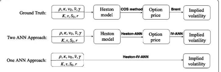
implied volatility, as presented in Fig.1. Using two separate ANNs to map the Heston
parameters to implied volatility has been applied in [26]. In the present paper, we merge
these two ANNs, see Fig.1. In other words, the Heston–IV–ANN is used as the forward
pass to learn the mapping between the model parameters and the implied volatility. Note that a similar model is employed for the Bates model, however then based on the Bates model parameters.
The forward pass consists of training and prediction, and in order to do so the network architecture and optimization method have to be defined. Generally, an increasing
ber of neurons, or a deeper structure, may lead to better approximations, but may also
result in a computationally heavy optimization and evaluation of the network. In [24] it is
proved that a deep NN can approximate a function for which a shallow NN may need a very large number of neurons to reach the same accuracy. Different residual neural networks have been trained and tested as a validation of our work. They may improve the predic-tive power while using a similar number of weights as in an MLP, but they typically take significantly more computing time during the training and testing phases. Very deep net-work structures may reduce the parallel efficiency, because the operations within a layer have to wait for the output of previous layers. With the limitation of computing resources available, a trade-off between ANN’s computation speed and approximation capacity may be considered.
Many techniques have been put forward to train ANNs, especially for deep networks.
Most of the neural network training relies on gradient-based methods. A properrandom
initializationmay ensure the network to start with suitable initial weight values.Batch normalizationscales the output of a layer by subtracting the batch mean and dividing it
by the batch standard deviation. This can often speed up the training process. Adropout
operationrandomly selects a proportion of the neurons and deactivates them, which forces the network to learn more generalized features and prevents over-fitting. The dropout rate
prefers to the proportion of deactivated neurons in a layer. In the testing phase, in order
to take into account the missing activation during training, each activation in the entire
network is reduced by a factorp. As a consequence, the ANNs prediction slows down,
which has been verified during experiments on GPUs. We found that our ANNs model did not encounter over-fitting even when using a zero dropout rate, as long as sufficient training data were provided. In our neural network we employ the Stochastic Gradient
Descent method, as further described in Sect.3.4.
3.3 The backward pass: calibration using ANNs
This section discusses the connection between training the ANN and calibrating the
fi-nancial model. First of all, both Equations (7) and (13) aim at estimating a set of
param-eters to minimize a particular objective function. For the calibration problem, these are the parameters of the financial model and the objective function is the error measure be-tween the market quantity and the model-based quantity. For the neural networks, the parameters correspond to the learnable weights and biases in the artificial neurons, and the objective function is the user-defined loss. This connection forms an inspiration for the machine learning-based approach to calibrate financial models.
As mentioned before, the ANN approach comprises three phases, training, prediction and calibration. During training, given the input-output pairs and a loss function as in
Equation (13), the hidden layers are optimized to determine the appropriate values of the
weights and biases, as shown in Fig.2(a), which results in a trained ANN approximating
the option solutions of the financial model (the forward pass, as explained in the previous section).
During the prediction phase, the hidden layers of the trained ANN are fixed (frozen), and new input parameters enter the ANN to yield the output quantities of interest. This phase is used to evaluate the performance of the trained ANN (the so-called model testing) or to accelerate option pricing by replacing the original solver.
During the calibration phase (orthe backward pass), the original input layer of the ANN
Figure 2The different phases of the CaNN
layers are the ANN layers obtained from the forward pass with the already trained weights,
as shown in Fig.2(b). By providing the output data, here consisting of market-observed
option prices and implied volatilities, and changing to an objective function for model
calibration, see Equation (7), the ANN can be used to find the input values that match the
given output. The task is thus to solve the inverse problem by learning a certain set of input
values, here the model parametersΘ, either for the Heston or Bates model. The option’s
strike priceK, as an example, belongs to the input layer, but is not estimated in this phase.
Note that the training phase in the forward pass is time-consuming but done off-line and only once. The calibration phase is computationally cheap, and is performed on-line. The calibration phase thus results in model parameters that best match the observed market data, provided the model has been trained sufficiently.
The gradients of the objective function, with respect to the input parameters, can be
de-rived based on Formula (10). This is useful when employing gradient-based optimization
algorithms to conduct model calibration with the trained ANNs. Compared to the classi-cal classi-calibration methods, in the ANN-based approach it is also possible to incorporate the gradient information from the trained ANNs to compute the search direction (without ex-ternal numerical techniques). As mentioned, we focus on a general calibration framework in which we can integrate both gradient-based and gradient-free algorithms. Importantly, within the proposed calibration framework we may insert any number of market quotes, without requiring a fixed structure of input parameters.
3.4 Optimization
The optimization method plays a key role in training ANNs and calibrating financial mod-els, but there are different requirements on the solutions for different phases. When train-ing the neural network to learn the mapptrain-ing between input and output values, we aim for a good performance on a test data set while optimizing the model on a training data set (this concept is called generalization). Calibration is regarded as an optimization problem with only a training data set, where the objective is to fit the market-observed prices as well as possible. In this work, the Stochastic Gradient Descent (SGD) is used when train-ing the ANN, and Differential Evolution is preferred in the phase of calibration to address
3.4.1 Stochastic gradient descent
A popular optimizer to train ANNs is SGD [30]. Neural networks contain thousands of
weights, which gives rise to a high-dimensional, non-convex optimization problem. The local minima appear not to be problematic for this involved black-box system, as long as
the cost function reaches a sufficiently low value. Optimization of Equation (6) based on
SGD is computed using,
⎧ ⎪ ⎪ ⎨ ⎪ ⎪ ⎩
W(i+1)←W(i)–η(i)∂L ∂W, b(i+1)←b(i)–η(i)∂L
∂b, fori= 0, 1, . . . ,NT,
whereLis a loss function as in Equation (12) andNTis the number of training iterations.
The bias and weights parameters are denoted byθ= (W, b). The loss function of training
the ANN solver is based on MSE in this paper.
In practice, the gradients are computed over mini-batches because of computer memory limitations. Instead of all input samples, a portion is randomly selected within each itera-tion to calculate an approximaitera-tion of the gradient of the objective funcitera-tion. The size of the mini-batch is used to determine the portion. Due to the architecture of the GPUs, batch sizes of powers of two can be efficiently implemented. Several variants of SGD have been
developed in the past decades, e.g., RMSprop and Adam [23], where the latter method
handles an optimization problem adaptively by adjusting the involved parameters over time.
3.4.2 Differential evolution
Differential Evolution (DE) [33] is a population-based, derivative-free optimization
algo-rithm, which does not require any specific initialization. With DE, a global optimum can be found, even when the objective function is non-convex. The general form of the DE algorithm usually comprises the following four steps:
1. Initialization: Generate the population withNpindividuals and locate each member
with random positions in the search space,
(θ1,θ2, . . . ,θNp).
2. Mutation: Once initialized, a randomly sampled difference is added to each individual, named differential mutation.
θi=θa+F·(θb–θc), (14)
whereirepresents theith candidate, and the indicesa,b,care randomly selected from the population witha=i. The resultingθis called a mutant. The differential weightF∈[0,∞)determines the step size of the evolution. Generally, largeFvalues increase the search radius, but may cause DE to converge slowly. There are several mutation strategies, for example, whenθais always the best candidate of the previous population, the mutation strategy is calledbest1bin, which will be used in the following numerical experiments; whenθais randomly chosen, it is calledrand1bin.
After this step, an intermediary (or donor) population, consisting ofNpmutant
3. Crossover: During the crossover stage, mutated candidates that may enter the next evaluation stage are determined. For eachi∈ {1, . . . ,Np}, a uniformly distributed
random numberpi∼U(0, 1)is selected. Some samples are filtered out by setting a
user-defined crossover possibilityCr∈[0, 1],
θi =
⎧ ⎨ ⎩
θi, ifpi≤Cr,
θi, otherwise. (15)
If the probability is greater thanCr, the donor candidate will be discarded. Increasing
Crallows more mutants to enter the next generation, but at the expense of population stability. Here, a trial population(θ1,θ2, . . . ,θNp)has been defined. 4. Selection: Comparing each new trial candidate with the corresponding target
individual on the objective function,
θi←
⎧ ⎨ ⎩
θi, ifg(θi)≤g(θi),
θi, otherwise.
(16)
If the trail individual has improved performance, the selected individual is replaced. Otherwise, the offspring individual inherits the parameters from its parent. This gives birth to a next generation population.
The Steps (2)–(4) are repeated until the algorithm converges or until a pre-defined crite-rion is satisfied. Adjusting the control parameters may impact the performance of DE. For example, a large population size and mutation rate can increase the probability of finding the global minimum. An additional parameter, convergence tolerance, is used to measure the diversity within a population, and determines when to stop DE. The control parame-ters can also change over time, which is out of our scope here.
3.4.3 Acceleration of calibration
In this section we develop DE into a parallel version which is beneficial within the ANNs. Generally, matrix multiplications and element-wise operations in a neural network can be implemented in parallel to reduce the computing time, especially when a large number of arguments is involved. As a result, several components of the calibration procedure can be accelerated. For the ANN solver in the forward pass, all observed market samples can be evaluated at once. Furthermore, in the selection stage of the DE, an entire population can be treated simultaneously. Note that the ANN solver runs in parallel, especially on any GPU.
An example of the parameter settings for DE is shown in Table1, where the population
of one generation comprises 50 vector candidates for the calibrated parameters (e.g., a
Table 1 The setting of DE
Parameter Option
vector candidate contains five parameters to calibrate in the Heston model), and each
candidate produces a number of market samples (here 35, i.e., 7 strike pricesKand 5 time
points). So, there are 50×35 = 1650 input samples for the Heston model each generation.
Traditionally, all these input samples (here 1650) are computed individually, except for
those with the same maturity timeT. The first speed-up is achieved because 35 sample
output quantities from each parameter candidate can be computed by the ANN solver at the same time, even if these samples have different maturity times and strike prices. The second speed-up is based on the parallel DE combined with the ANN, where all parameter candidates in one generation enter the ANN solver at once, that is, all 1650 input samples in one generation can be included in the ANN solver simultaneously, giving 1650 output values (e.g., implied volatilities). Note that the batch size of the ANN solver should be adapted to the limitations of the specific processor, here 2048 in our used processor. We find that with the population size being around 50, the parallel CaNN is at least 10 times faster than the conventional CaNN, on either a CPU or a GPU. It is believed that a larger population size should lead to a higher parallel computing performance, especially on a GPU.
Remark There are basically two error sources in this framework. One is a consistency error which comes from the employed numerical methods to solve the financial model, and it is found while generating the training data set. The other is an optimization error during training and calibration. These errors will influence the performance of the CaNN.
4 Numerical results
In this section we show the performance of the proposed CaNN. We begin with calibrating the Heston model, a special case of the Bates model. Some insights into the effect of the Heston parameters on the implied volatility are discussed to give some intuition on the re-lation, since no explicit mapping between them exists. Then, the forward pass is presented where an ANN is trained to build a mapping between the model parameters and implied volatilities. It is also demonstrated that the trained forward pass can be used as a tool for performing the sensitivity analysis of the model parameters. After that, we implement the backward pass of the Heston–CaNN to calibrate the model and evaluate the CaNN per-formance. We end this section by considering the calibration of the Bates model, a model that consists of more parameters than the Heston model, using the Bates–CaNN.
4.1 Parameter sensitivities for Heston model
This section discusses the sensitivity of the implied volatility to the Heston coefficients. This sensitivity analysis can be used to estimate a set of initial parameters, as is used in tra-ditional calibration methods. In our calibration method this will not be required, however, we can gain some insights in the case of no explicit formulas.
The typically observed implied volatility shapes in the market, e.g., the implied volatility smile or skew, can be reproduced by varying the above parameters{κ,ρ,γ,ν0,ν¯}. We will
give some intuition about the parameter values and their impact on the implied volatil-ity shape. From a PDE viewpoint, the calibration problem consists of finding appropriate values of PDE coefficients{κ,ρ,γ,ν0,ν¯}to make the Heston model to reproduce the
ob-served option/implied volatility data. The authors in [12] reduce the calibration time by
the Heston dynamics was employed to determine a satisfactory initial set of parameters,
followed by a local optimization to reach the final parameters. The paper [6] derived a
Heston model characteristic function to analytically obtain gradient information of the
option prices during the search for an optimal solution. In Sect.4.3.2we will use the ANN
to extract gradient information of the implied volatility with respect to the Heston param-eters.
4.1.1 Effect of individual parameters
To analyze the parameter effects numerically, we use the following set of reference param-eters,
T= 2, S0= 100, κ= 0.1, γ = 0.1,
¯
ν= 0.1, ρ= –0.75, ν0= 0.05, r= 0.05.
A numerical study is performed by varying individual parameters while keeping the oth-ers fixed. For each parameter set, Heston stochastic volatility option prices are computed (by means of the numerical solution of the Heston PDE) and the Black–Scholes implied volatilities are subsequently determined.
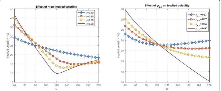
Two important parameters that are varied are the correlation parameter ρ and the
volatility-of-variance parameterγ. Figure3(left side) shows that, whenρ= 0%, an
in-creasing value ofγ gives a more pronounced implied volatilitysmile. A higher
volatility-of-variance parameter thus increases the implied volatilitycurvature. We also see, in Fig.3
(right side), that when the correlation between stock and variance process gets
increas-ingly negative, the slope of theskewin the implied volatility curve increases. Furthermore,
it is found that parameterκhas a limited effect on the implied volatility smile or skew, up
to 1%–2%only. It determines the speed at which the volatility converges to the long-term
volatilityν¯.
The optimization can be accelerated by a reduction of the set of parameters to be
opti-mized. By comparing the impact of the speed of mean reversion parameterκand the
cur-vature parameterγ, it is observed that these two parameters have a similar effect on the
shape of the implied volatility. It is therefore common (industrial) practice to prescribe (or
fix) one of them. Practitioners often fixκand optimize parameterγ, for exampleκ= 0.5. By this, the optimization reduces to four parameters.
Another parameter which may be determined in advance, using heuristics, is the initial
value of the variance processν0. For maturity timeT “close to today” (i.e.,T →0), one
expects the stock price to behavelike in the Black–Scholes case. The impact of a stochastic
variance process should reduce to zero, in the limitT→0. For options with short
matu-rities, the process may therefore be approximated by a process of the following form:
dS(t) =rS(t)dt+√ν0S(t)dWx(t). (17)
This suggests that for initial varianceν0one may use the square of the ATM implied
volatil-ity of an option with the shortest maturvolatil-ity,ν0≈σimp2 , forT→0, as an accurate
approxima-tion for the initial guess for the parameter. One may also use the connecapproxima-tion of the Heston dynamics to the Black–Scholes dynamics with a time-dependent volatility function. In the
Heston model we may, for example,projectthe variance process onto its expectation, i.e.,
dS(t) =rS(t)dt+Eν(t)S(t)dWx(t).
By this projection the parameters of the variance processν(t) may be calibrated similar
to the case of the time-dependent Black–Scholes model. The Heston parameters are then determined, such that
σATM(Ti) =
Ti
0
Eν(t)2dt,
whereσATM(Ti) is the ATM implied volatility for maturityTi.
Another classical calibration technique for the Heston parameters is to use VIX index
market quotes. With different market quotes for different strike pricesKiand for different
maturitiesTj, we may determine the optimal parameters by solving the following
equali-ties, for all pairs (i,j),
Ki,j=ν¯+
ν0–ν¯
κ(Tj–t0)
1 –e–κ(Ti–t0). (18)
When the initial values of the parameters have been determined, one can use the whole implied volatility surface to determine the optimal model parameters. To conclude, the number of the Heston parameter to be calibrated depends on different scenarios. The flexibility of our CaNN is that it can handle varying numbers of to-calibrate parameters.
4.1.2 Effect of two combined parameters
In this section, two parameters are varied simultaneously in order to understand the joint
impact on the objective function. Figure4(a) presents the landscape of the objective
func-tion, here the logarithm of the MSE, when varyingν0andκbut keeping the other
parame-ters fixed in the Heston model. It is observed that the valley is narrow in the direction ofν0
but flat in the direction ofκ. Several values of these parameters thus result in similar
Figure 4Landscape of the objective function for the implied volatility. The true values areκ∗= 1.0 and ν0∗= 0.2 in the left plot, andκ∗= 1.0 andν¯∗= 0.2 in the right plot. There are 35 market samples. The objective
function is MSE. The contour plot is rendered by a log-transformation
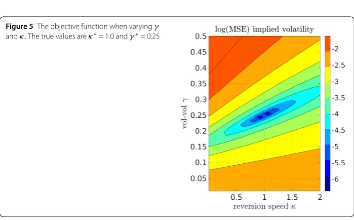
Figure 5The objective function when varyingγ andκ. The true values areκ∗= 1.0 andγ∗= 0.25
above a certain error threshold. Furthermore, forν¯andκwe observe also a flat minimum,
with multiple local minima giving rise to similar MSEs, see Fig.4(b).
A similar observation holds forκ andγ: small values ofκ and largeγ values will, in
certain settings, give essentially the same option prices as large values ofκ and smallγ
values. This may give rise to multiple local minima for the objective function, as shown in Fig.5.
4.2 The forward pass
In this section, we discuss the forward pass, i.e., Heston–IV–ANN. A relatively large neural network is chosen so that in the forward pass the network is overparametrized in terms of its expressive power and should be able to fit the pricing model well enough. This in turn comes at the cost of a more expensive computation, but provides a suitable forward
pass to demonstrate that the parallel backward pass, in Sect.4.3, can handle
computation-intensive model calibration in a fast way. The selected hyper-parameters are listed in
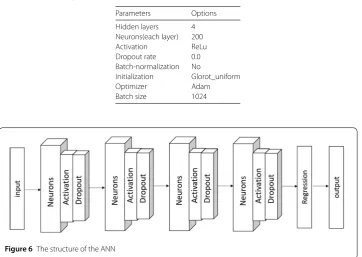
Ta-ble2. Please note that increasing the number of neurons or using a deeper structure may
lead to better approximations, but gives rise to an expensive-to-compute network. With our computing resources, we choose to employ 200 neurons each hidden layer to balance the calibration speed and accuracy. We use 4 hidden layers and a linear output (regres-sion) layer, so that the network contains 122,601 trainable parameters. MSE is used as the
loss function measure to train the forward pass. The global structure is depicted in Fig.6.
More details on the ANN solver can be founded in [26].
As a data-driven method, the samples from the parameter set for which the ANN is trained are randomly generated for the pricing of European options. The input contains eight variables, and Table3presents the range of six Heston input parameters (r,ρ,κ,ν¯,γ,
ν0) as well as two option contract-related parameters (τ,m), with a fixed strike priceK= 1.
There are around one million data points. The complete data set is randomly divided into three parts, with 10% as the testing set, 10% as validation and 80% as the training data set. After sampling the parameters, a robust version of the COS method is used to determine
the option prices under the Heston model numerically. The default setting withLCOS= 50
andNCOS= 1500 will provide highly accurate option solutions for most of the samples,
but it may end up with insufficient precision in some extreme parameter cases. In such cases, the integration interval [a,b] will be enlarged automatically, by increasingLCOSuntil
Table 2 Details and parameters of the selected ANN
Parameters Options
Hidden layers 4 Neurons(each layer) 200 Activation ReLu Dropout rate 0.0 Batch-normalization No
Initialization Glorot_uniform Optimizer Adam Batch size 1024
Table 3 Sampling range for the Heston parameters. LHS means Latin Hypercube Sampling, COS stands for the COS method (see theAppendix) and Brent for the root-finding iteration
ANN Parameters Value range Generating method
ANN Input Moneyness,m=S0/K [0.6, 1.4] LHS
Time to maturity,τ [0.05, 3.0] (year) LHS Risk free rate,r [0.0%, 5%] LHS Correlation,ρ [–0.90, 0.0] LHS Reversion speed,κ (0, 3.0] LHS Volatility of volatility,γ (0.01, 0.8] LHS Long average variance,ν¯ (0.01, 0.5] LHS Initial variance,ν0 (0.05, 0.5] LHS
– European put price,V (0, 0.6) COS ANN Output Black–Scholes IV,σ (0, 0.76) Brent
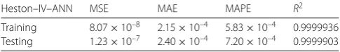
Table 4 The trained forward pass performance. The default float type is float32 on the GPU. The measures are defined as follows: MSE =1n(yi–yˆi)2, MAE =n1
|yi–ˆyi|, MAPE =1n |yi–ˆyi|
yi , wherey represents the true value, andyˆrepresents the predicted value withnbeing the number of samples
Heston–IV–ANN MSE MAE MAPE R2
Training 8.07×10⁻⁸ 2.15×10⁻⁴ 5.83×10⁻⁴ 0.9999936
Testing 1.23×10⁻⁷ 2.40×10⁻⁴ 7.20×10⁻⁴ 0.9999903
the lower boundaand the upper boundbhave different signs. Subsequently, the Black–
Scholes implied volatility is calculated by Brent’s method.
The option prices are just intermediate variables during training in the forward pass. The overall Heston–IV–ANN solver does not depend on the type of European option (e.g., call or put), since during the computation of the Black–Scholes implied volatilities the European options with identical Heston parameters should give rise to the same implied volatilities, independent of call or put prices. The forward pass can handle both call and put implied volatilities without requiring additional efforts. Here we are using European put options, since the COS method is more robust for pricing put than call options.
The ANN takes as input parameters (r,ρ,κ,ν¯,γ,ν0,τ,m), and approximates the Black–
Scholes implied volatilityσ. As mentioned in Table2, the optimizer Adam is used to train
the ANN on the generated data set. The learning rate is halved every 500 epochs. The training consists of 8000 epochs, both the training and validation losses have converged.
The performance of the trained model is shown in Table4.
We observe that the forward pass is able to obtain a very good accuracy and therefore learns the mapping between model parameters and implied volatility in a robust and ac-curate manner. The test performance is very similar to the train performance, showing that the ANN is able to generalize well.
4.3 The backward pass
We will perform calibration using the CaNN based on the trained ANN from the previous section and evaluate its performance. We will work with the full set of Heston parameters to calibrate, but we will also study the impact of reducing the number of parameters to calibrate, as discussed in Sect.4.1.1.
The aim is to check how accurately and efficiently the ANN approach can recover the in-put values. In order to investigate the performance of the proposed calibration approach,
Figure 7The Calibration Neural Network for the Heston model
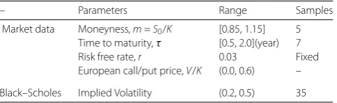
Table 5 The range of market quotes
– Parameters Range Samples
Market data Moneyness,m=S0/K [0.85, 1.15] 5
Time to maturity,τ [0.5, 2.0](year) 7 Risk free rate,r 0.03 Fixed European call/put price,V/K (0.0, 0.6) –
Black–Scholes Implied Volatility (0.2, 0.5) 35
where the ‘true’ values of the parameters are known in advance. In other words, the pa-rameters used to obtain the IV’s from the COS-Brent’s method, are now taken as
out-put of the backward pass of the neural network, with σimp being the input conditional
on (K,τ,S0,r). Different financial models correspond to different CaNNs. Here we
distin-guish the Heston–CaNN (based on the Heston model, studied in this section), from the
Bates–CaNN (based on the Bates model, studied in Sect.4.3.3).
There are 5×7 = 35 ‘observed’ European option prices, that are made up of European
OTM puts and calls. As shown in Table5, the moneyness ranges from 0.85 to 1.15, and
the maturity times vary from 0.5 to 2.0. Each implied volatility surface contains money-ness levels (85%, 90%, 95%, 100%, 110%, 115%) and maturities (0.5, 0.75, 1, 1.25, 1.5, 1.75,
2.0) with a prescribed risk-free interest rate of 3%. The samples withm< 1 correspond to
European call OTM options, while those ones withm> 1 andm= 1 are OTM and ATM
put options, respectively.
We use the total squared error measureJ(Θ) as the objective function during the
cali-bration,
J(Θ) =ωσimpANN–σimp∗ 2+λ¯Θ, (19)
where σimpANN is the ANN-model-based value andσimp∗ is the observed one. We give a
small penalty parameterλ¯depending on the dimensionality of the calibration.dThe
for-ward pass has been trained with implied volatility as the output quantity, as described in
Sect.4.1.2. The parameter settings of the DE optimization is shown in Table1.
4.3.1 Calibration to Heston option quotes
In this section we focus on two scenarios for the Heston model, calibrating either three
parameters, with a fixedκand a knownν0, or calibrating five parameters. In order to
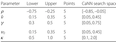
cre-ate synthetic calibration data, we choose five equally-spaced points between the lower and
upper bound for each parameter, and there are 55= 3125 combination cases in total, as
be-Table 6 Uniformly distributed points between the lower and upper bounds of the Heston parameters
Parameter Lower Upper Points CaNN search space
ρ –0.75 –0.25 5 [–0.85, –0.05]
¯
ν 0.15 0.35 5 [0.05, 0.45]
γ 0.3 0.5 5 [0.05, 0.75]
ν0 0.15 0.35 5 [0.05, 0.45]
κ 0.5 1.0 5 [0.1, 2.0]
Table 7 Averaged performance of the backward pass of the Heston–CaNN, calibrating3parameters on a CPU (Intel i5, 3.33 GHz with cache size 4 MB) and on a GPU (NVIDIA Tesla P100), over 3125×5 (random seeds) test cases, where†stands for CaNN estimated value, and∗stands for the true value, with MJ =J(Θ)/N
Absolute deviation fromΘ∗ Error measure Computational cost
|¯v†–v¯∗| 1.60×10⁻³ J(Θ) 1.45×10⁻⁶ CPUtime (seconds) 0.29 |γ†–γ∗| 1.79×10⁻² MJ 4.14×10⁻⁸ GPUtime (seconds) 0.15 |ρ†–ρ∗| 2.44×10⁻² Data points 35 Function evaluations 59,221
Table 8 Performance of Heston–CaNN calibrating5parameters on a GPU over 3125×5 (random seeds) test cases
Absolute deviation fromΘ∗ Error measure Computational cost
|ν0†–ν0∗| 4.39×10⁻⁴ J(Θ) 2.52×10⁻⁶ CPU time (seconds) 0.85 |¯ν†–ν¯∗| 4.54×10⁻³ MJ 7.18×10⁻⁸ GPU time (seconds) 0.48 |γ†–γ∗| 3.28×10⁻² Function evaluations 193249
|ρ†–ρ∗| 4.84×10⁻² Data points 35
|κ†–κ∗| 4.88×10⁻²
cause the DE optimization involves random operations which may cause the performance
to fluctuate. In addition, all quotes have the equal weightω= 1 in this section.
First, the scenario of three parameters is studied, fixingκ andν0 during calibration.
We compare the averaged results by implementing each test case five times. The wording “function evaluation” refers to how many times the model has been compared to the ob-served implied volatility. The population size in the DE is 15×Nv, that is, 15×3 = 45. With
the population ratio increasing further, no significant benefits were observed. As shown
in Table7, the time on the GPU is around half of that on the CPU.
In the case of five parameters (ρ,ν¯,γ,ν0,κ), the calibration problem is more likely to give
rise to a many-to-one problem; that is, many sets of parameter values may correspond to
the same volatility surface. A regularization factorλ¯= 1.0×10⁻⁶is added to guide CaNN
to a set of values for which the sum of their magnitude is the smallest among the feasible
solutions, as shown in Equation (6). Here the DE population size is 50 = 10×5 parameters.
As shown in Table8, the Heston–CaNN finds the values of these parameters in
approxi-mately 0.5 seconds on a GPU, with around 20,000 function evaluations.There are several
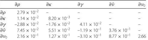
Table 9 A Hessian matrix at the true value setΘ∗
∂ρ ∂κ ∂γ ∂ν¯ ∂ν0
∂ρ 2.79×10⁻² – – – –
∂κ 1.14×10⁻² 8.20×10⁻³ – – –
∂γ –2.88×10⁻² –1.76×10⁻² 4.11×10⁻² – –
∂ν¯ 7.45×10⁻² 5.51×10⁻² –1.19×10⁻¹ 3.76×10⁻¹ –
∂ν0 2.16×10⁻¹ 1.27×10⁻¹ –3.10×10⁻¹ 8.77×10⁻¹ 2.66
4.3.2 Sensitivity analysis based on ANNs
The gradients of the objective function can be extracted from the trained model, as
men-tioned in Sect.3.1. These can be used to gain some insights into the complex structure of
the loss surface and thus into the complexity of the optimization problem for calibration. We use here the Hessian matrix, which describes the local curvature of the loss function. No explicit formula is available for the relations the neural network learns between the implied volatilities and the model parameters, however, it is feasible to extract the
Hes-sian from the trained ANN, giving insight into this relation and the sensitivities. Table9
shows a Hessian matrix, where the Hessian is defined as ∂yiyjL(Θ), where yi andyj are
output of the neural network (y∈Θ, the to-be calibrated parameters). The Hessian is
computed by differentiating the Heston–IV–ANN loss for computing the Black–Scholes implied volatility with respect to the Heston parameters on 35 market data points based
on the parameter ranges in Table5. Here the objective function is the MSE to exclude the
effects of a regularization factor.
We can understand how the parameters affect the loss surface around the optimum with help of the Hessian matrix, by analyzing the sensitivities of the implied volatility with
re-spect to the five parameters. Observe that the value of the Hessian with rere-spect toκ is
the smallest among the sensitivities. As shown in Table9, the ratio between∂2J(Θ∗)/∂ν02
and∂2J(Θ∗)/∂κ2is around 323, which suggests that changing 1 unit ofν
0is approximately
equivalent to changing 323 units ofκfor the objective function. When the Hessian value
is small in absolute value, the loss surface at that point exhibits flatness in the
correspond-ing direction. As visible in Fig.4, the ground-truth loss surface gets increasingly stretched
along the axis withκ, resulting in a narrow valley with a flat bottom. This also indicates that there is no unique global minimum above a certain non-zero convergence tolerance, since
multiple values ofκwould result in similar values of the loss function. In addition, the
con-vergence performance, especially for the steepest descent method, depends on the ratio of the smallest to the largest eigenvalue of the Hessian; this ratio is also known as the con-dition number in the case of symmetric positive matrices. The ratio between∂2J(Θ∗)/∂ν¯2
and∂2J(Θ∗)/∂κ2is around 45, as visible in Fig.4(b). From the results in [6], when the
tar-get quantity is based on the option prices, this ratio between∂2J(Θ∗)/∂ν¯2and∂2J(Θ∗)/∂κ2
is sometimes found to be of order 106, which makes the calibration problem increasingly
complex due to a great disparity in sensitivity. Calibrating to the implied volatility appears to reduce the ratio between different Hessian entries compared to the option prices, thus decreasing Hessian’s condition number and resulting in a more efficient and accurate cal-ibration performance.
significantly. A straightforward way to address this issue is by adding a regularization term
to choose a particular solution, for example, like Equation (19). Another way is to take
advantage of the population-based algorithm DE. Since there are several candidates in each generation, we can select the top few candidates to get an averaged solution when DE converges. This averaged solution may lead to wider optima and better robustness.
Some recent papers, like [21] have used similar ideas to improve the generalization of the
neural network. The parameterν0is the most sensitive one and it appears to dominate
the ANN calibration process. Therefore, the predicted parameterν0is the most precise
among all parameters in order to achieve the desired accuracy.
The above analysis explains the behavior of the absolute deviation of the five parameters
as shown in Table8. The error measure MJ can not drop significantly below 7.18×10⁻⁸,
as this value is close to the testing accuracy, MSE = 1.23×10⁻⁷, of the Heston–IV–ANN
model. In other words, any further exploration of the DE optimization can not distinguish the parameters impact on the loss anymore.
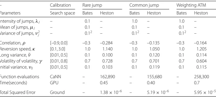
4.3.3 Calibration to Bates quotes
In this section, we use the Bates model to create the synthetic market data, in order to generate a more realistic (complex) volatility shape by adding some ‘perturbations’ to the previous Heston data. It is then followed by a calibration based on the Heston model. The aim is to check whether the resulting implied volatilities can be recovered by the machine learning calibration framework.
So, the observed data set in Table10is from the Bates option prices. During the
calibra-tion, we will employ the backward pass based on the Heston model to determine a set of parameter values which approximate the generated implied volatility function.
There are two sets of experiments, based on either rare jumps or common jumps in the
stock price process. Figure8compares the implied volatility from the Bates model
(for-ward) computations and the CaNN-based Heston implied volatilities. Clearly, when the impact of the jumps is small, the Heston model can accurately mimic the implied volatility generated by the Bates parameters. In this case, many different input parameters for the
Table 10 The Heston parameters are estimated with the CaNN by calibrating to a data set generated by the Bates model. ‘Ground total squared error’ refers to the sum of the differences betweenσimp∗
andσimp, whereσimpis obtained using the COS and Brent methods with already calibrated Heston
parameter values. For a single calibration case, the computing time fluctuates slightly, as the CPU or GPU performance may be influenced by external factors. Function evaluations should be a reliable measure to estimate the time
– Calibration Rare jump Common jump Weighting ATM
Parameters Search space Bates Heston Bates Heston Bates Heston
Intensity of jumps,λJ – 0.1 – 1.0 – 1.0 –
Mean of jumps,μJ – 0.1 – 0.1 – 0.1 –
Variance of jumps,ν2
J – 0.1
2 – 0.12 – 0.12 –
Correlation,ρ [–0.9, 0.0] –0.3 –0.284 –0.3 –0.135 –0.3 –0.164 Reversion speed,κ [0.1, 3.0] 1.0 1.140 1.0 1.050 1.0 1.205 Long variance,ν¯ [0.01, 0.5] 0.1 0.100 0.1 0.120 0.1 0.114 Volatility of volatility,γ [0.01, 0.8] 0.7 0.728 0.7 0.701 0.7 0.604 Initial variance,ν0 [0.01, 0.5] 0.1 0.103 0.1 0.119 0.1 0.115
Function evaluations CaNN – 162,890 – 155,680 – 258,300
Time(seconds) GPU – 0.45 – 0.40 – 0.7
Figure 8Implied volatilities from the ‘market’ and calibration. The solid lines represent the Bates implied volatilities, while the dashed lines are the calibrated Heston-based volatilities. The impact of weighting ATM options can be seen in the third figure
Bates model will give very similar implied volatility surfaces. With an increasing jump in-tensity, the deviation between the two models can become significant, especially for short maturity options.
In financial practice, a perfect calibration to the ATM options is often required. We can enforce this, by increasing the weights of the ATM options in the objective function.
The third figure from Fig.8and Table10compare the differences when weighting ATM
options in the objective function. The two curves fit very well ATM, however, in this case the total error increases with unequal weighting. The results demonstrate the robustness of the CaNN framework. It is however well-known that the Heston model can not fit short-maturity market implied volatility very well, and therefore we will also employ a higher-dimensional model, e.g., calibrating directly the Bates model, which will be discussed in Sect.4.4.
4.4 Calibrating the Bates model
In this section, we show the ability of Bates–CaNN to calibrate the Bates model parame-ters. The Bates model calibration is a higher-dimensional problem, since the Bates model is based on more parameters than the Heston model. The proposed CaNN framework is used to calibrate eight parameters in the Bates model, a setting in which we are dealing with more complex implied volatility surfaces.
Table 11 The Bates parameters are estimated with Bates–CaNN, by calibrating to a data set (35 samples) generated by the Bates model. In DE, the random seed is 2 and the population size is 10×Nv= 80
Parameters CaNN search space Bates Calibrated
Intensity of jumps,λJ [0, 3.0] 1.0 1.065 Mean of jumps,μJ [0, 0.4] 0.1 0.087 Variance of jumps,ν2
J [0, 0.3] 0.160 0.146 Correlation,ρ [–0.9, 0.0] –0.3 –0.228 Reversion speed,κ [0.1, 3.0] 1.0 0.598 Long average variance,ν¯ [0.01, 0.5] 0.1 0.128 Volatility of volatility,γ [0.01, 0.8] 0.7 0.776 Initial variance,ν0 [0.01, 0.5] 0.1 0.102
Total Squared Error – – 4.95×10⁻⁶
Function evaluation – – 842,800
Time (seconds) – – 1.8
Figure 9The solid lines represent the observed implied volatilities, with the dashed lines being the model calibrated ones. This plot shows the result with equal weights andλ¯= 1.0×10⁻⁶. The random
seed is 2 during calibration
pass of the Heston model, merely a different characteristic function is inserted in the COS method, and three additional model parameters have been varied. The Bates–CaNN is employed to calibrate the Bates model, aiming to recover the eight Bates model parameters
possibly well. All the samples have equal weight, and the regularization factor isλ¯= 1.0×
10–6.
Table11shows an example with high intensity, large variance jumps, for which the
He-ston model can not capture the corresponding implied volatility accurately. There are still
35 market samples as shown in Table5. Estimating eight parameters is a challenging task,
including millions of comparisons between the model and the market values during cali-bration.
Figure9compares the implied volatilities from the synthetic market and the calibrated
Bates model. These volatilities resemble each other very well, even when the curvature is high with short time to maturity.
5 Conclusion