Efficient frequency-transient co-simulation of coupled heat-electromagnetic problems

R E S E A R C H

Open Access

Efficient frequency-transient co-simulation of

coupled heat-electromagnetic problems

Christof Kaufmann

_{, Michael Günther}

_{, Daniel Klagges}

_{, Michael Knorrenschild}

_{, Matthias Richwin}

_,

Sebastian Schöps

_{and E Jan W ter Maten}

*_{Correspondence:}

[email protected] 1_{Fachbereich Elektrotechnik und} Informatik, Hochschule Bochum, Bochum, 44801, Germany Full list of author information is available at the end of the article

Abstract

Background:With the recent advent of inductive charging systems all major automotive manufacturers develop concepts to wirelessly charge electric vehicles. Efficient designs require virtual prototyping that accounts for electromagnetic and thermal fields. The coupled simulations can be computationally very costly. This is because of the high frequencies in the electromagnetic part. This paper derives a mixed frequency-transient model as approximation to the original problem. We propose a co-simulation such that the electromagnetic part is simulated in the frequency domain while the thermal part remains in time domain.

Results:The iteration scheme for the frequency-transient model is convergent for high frequency excitation. The error bound improves quadratically with increasing frequency.

Conclusions:The frequency-transient model is very efficient for coupled heat-electromagnetic simulations since the time scales typically differ by several orders of magnitude. The time steps of the full system can be chosen according to the heat subsystem only.

MSC: 35K05; 35Q61; 65Z05; 78A25; 78M12; 80M25

Keywords: inductive charging; coupled simulation; co-simulation; electromagnetic; heat; modelling; dynamic iteration

1 Introduction

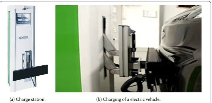
With the recent advent of inductive power charging systems and wireless power transmis-sion in consumer and mobile phone technology, [], all major automotive manufacturers develop concepts to wirelessly charge electric vehicles, both plug-in and pure electric ve-hicles (EV). For example the prototype from the Leopold Kostal GmbH & Co. KG of such an inductive charging station is shown in Figure . The necessity to charge EVs with to-day’s battery technology after every prolonged use - at least every night - is seen as one of the major drawbacks in the usability of EVs. A system to automate the charging process would reduce the burden on the driver; it could increase the acceptance of EVs, and, in the case of plug-in hybrid EVs, it could help to further reduce the COfootprint since the battery of the plug-in hybrid could always be considered fully charged. This is important for the calculation of the fleet COemission.

A future inductive charging system does not necessarily exhibit a lower efficiency than a comparable conductive charging system, since there are only a few additional

(a) Charge station. (b) Charging of a electric vehicle.

Figure 1 Prototype of an inductive charging station that charges the vehicle through its number plate (Images from Leopold Kostal GmbH & Co. KG).

nents; in a simplified view, the inductive charging system could be considered as a con-ductive charging system that has been cut in half in the middle of the transformer. There are, however, certain aspects that require attention and detailed design and optimization. These include positioning tolerances of the stationary (‘primary’) and car-mounted (‘sec-ondary’) coils, magnetic stray fields, and thermal aspects.

The efficiency of both conductive and inductive charging systems is aimed well above %, measured from the primary AC connection to the drive train battery. But even with this high efficiency, at . kW of first generation systems charging power there is a non-negligible amount of heat to be dissipated. Later generations with even higher power will further increase the heat load on the components. This heat load is the result of several different processes, namely resistance losses due to DC resistance and proximity effects, ferrite core losses and switching losses in the active semiconductor switching components. The main effects appear at the same frequency range as the magnetic field, which is of the order of - kHz. The resulting temperature however changes on much slower timescales, in the order of minutes, determined by the heat capacity and the (relatively large) mass of the involved components. This electromagnetic-thermal problem is fully coupled, as many of the material parameters show a significant thermal dependence. Typ-ical ferrite core losses, for instance, are minimal at temperatures around ◦C and increase below and above this temperature. This drives the equilibrium temperature of the ferrite material always close to this temperature, if the dissipated power is small enough, or makes the system thermally unstable, if the heat power is too high.

Engineering samples of such systems are expensive, heavy, possibly dangerous to oper-ate, and take a lot of time to build and optimize. Virtual prototyping using efficient sim-ulation methods accelerates this process. There are different methodologies and models available, [].

con-vergence properties in Section . The analysis exhibits interesting results, especially for high frequencies. Possibilities to generalize this model are also discussed. Section  vali-dates the results by a numerical simulation of a simplified model of the inductive charging system shown in Figure .

In contrast to [], where the different ways of co-simulation are discussed, we focus here on modeling and analysis of thefrequency-transient model.

2 Modeling

In this section, we derive a model, which describes the electromagnetic field coupled to the temperature in the materials. For that, in Section . Maxwell’s equations are intro-duced with temperature dependent material parameters. The conduction of the heat is described in Section . by the heat equation together with an electromagnetic power term as source to describe the Joule losses of the EM field. Finally, in Section . assump-tions and approximaassump-tions lead to thefrequency-transient model[].

2.1 Maxwell’s equations Maxwell’s equations read

∇ ·D=ρ, ()

∇ ·B= , ()

∇ ×E= –∂B

∂t, ()

∇ ×H=∂D

∂t +J, ()

whereEandHare the electric and magnetic field strength,DandBare the electric and magnetic flux densities,ρandJare the electric charge and current densities. These laws are supported by the constitutive relations

D=εE, B=μH and J=σ(T)E+Jsrc,

where the permittivityεand permeabilityμparameters depend only on space while the conductivityσ may also depend on the temperatureT. In this way the EM field solution is a function of the temperature distribution (parameter coupling). However, the source current densityJsrcdescribes an external excitation [, ]; it is assumed to be independent of the temperature. Now to reduce the unknowns in Maxwell’s equations, we introduce the magnetic vector potentialAand the electric scalar potentialϕas

E= –∇ϕ–∂A

∂t withB=∇ ×A.

By using these potentials, () and () are fulfilled automatically. From () we get

∇ ×μ–∇ ×A+ε∂

_A

∂t +σ(T)

∂A

∂t +ε∇

∂ϕ

∂t +σ(T)∇ϕ=Jsrc.

With Buchholz gauge transformation (∇ϕ= ) this reduces to

∇ ×μ–∇ ×A+ε∂

_A

∂t +σ(T)

∂A

The so-called curl-curl equation will be treated in the following on a finite domain with adequate boundary conditions (BC) and initial values (IV).

For the low frequency range, where inductive effects dominate, usually the displacement current∂D/∂t=ˆωεAˆ can be disregarded. This is called magnetoquasistatic formulation. For details on these formulations we refer to []. Here we are interested in the high fre-quency range. Therefore our model is based on the full Maxwell formulation ()-().

2.2 Heat equation

The classical heat equation describes conduction of heat in materials:

ρc∂T

∂t =∇ ·(k∇T) +Q ()

with heat conductivityk, densityρand specific heat capacityc, all constant in time and again on a finite domain with BC and IV. The termQrepresents the Joule losses of the EM field. Hence we use a source coupling to connect the heat equation with the EM curl-curl equation (). For simplicity we consider only eddy-current and Joule losses and thus obtain

Q(A,T) =J·E=σ(T)E·E+Jsrc·E=σ(T)

∂A

∂t ·

∂A

∂t –Jsrc·

∂A

∂t. ()

The power term is further simplified in the next section.

2.3 Frequency-transient model

Now we aim at a model which allows an efficient simulation. The model consisting of () and () with () is defined in the time domain. A multirate co-simulation scheme could simulate both equations with different time steps. However, for a fast varying source cur-rent density the main part of the computational costs is caused by the simulation of (). A discussion of single-rate and multirate schemes can be found in []. We will reduce these costs further by refining the model.

Since the temperature is only slowly varying in comparison to the EM field in () the temperatureT, whereσis evaluated at, can be averaged by

˜ Ti:=



τi+–τi

τi+

τi

T(t)dt.

Thus we useσ(T(t))≈σ(T˜i) fort∈[τi,τi+] and then () can be approximated by

∇ ×μ–∇ ×A+ε∂

_A

∂t +σ(T˜i)

∂A

∂t =Jsrc. ()

However, this is still in time domain. To allow a solution in frequency domain, we assume a time harmonic source current density

Jsrc=  ˆJsrce

jωt₊ ˆJsrce

–jωt_{, ()}

whereˆJsrcis a complex phasor. It follows forμandεindependent ofAthat

A(t) =  

_ˆ

where the complex phasorAˆcis the solution forˆJsrc. This means the amplitude is constant within the time interval [τi,τi+].

Let us look at () again, but now with the approximationσ(T(t))≈σ(T˜i). The dot prod-uct is the usual real inner prodprod-uct.

Q(A,T˜i) =σ(T˜i)∂A

∂t ·

∂A

∂t –Jsrc·

∂A

∂t

= –σ(T˜i)ω 



_ˆ

Ac· ˆAcejωt– Aˆc· ˆAc+Aˆc· ˆAce–jωt

–jω



_ˆ

Jsrc· ˆAcejωt–ˆJsrc· ˆAc+Jˆsrc· ˆAc–ˆJsrc· ˆAce–jωt

,

where Aˆ_c=Aˆ_c(T˜i). Now we are interested in the mean power loss in the time interval [τi,τi+]:

˜ Qi:=



τi+–τi

τi+

τi

QA(t),T˜i

dt ()

and thus all parts withe±jωt_{vanish (for interval length being a multiple of the half period} length, i.e.τi+–τi=cπω, wherec∈N). Then we are left with

˜

Qi=σ(T˜i)

ω

 Aˆc(T˜i)  c+

ω

Im

_ˆ

Jsrc· ˆAc(T˜i)

, ()

where Ac:=A·Ais the Euclidean norm for complex vectorsA. Now the simplified curl-curl equation () can be considered in frequency domain (with vector potentialAˆc=

ˆ

Ac(T˜i)) along with the simplified heat equation () left in time domain:

jωσ(T˜i) –ωεAˆc+∇ ×

μ–∇ × ˆAc

=ˆJsrc, ()

ρc∂T

∂t =∇ ·(k∇T) +Q˜i. ()

The curl-curl equation is formulated with constant material parameters in frequency domain. Thus, only a linear, complex system has to be solved once for each time window, instead for each time step of the curl-curl equation in time domain.

3 Algorithm

We will now discuss the algorithm to simulate heat-EM problems with the frequency-transient model. After discretization, the model is solved in a Gauss-Seidel scheme, which can be interpreted as co-simulation. It is comparable with a dynamic iteration for time integration. Section . will briefly discuss the co-simulation scheme. In Section . the convergence analysis for the iteration is proved.

3.1 Method

drawback of non-diagonal material matrices. This would complicate the following deriva-tions. However, in FIT-notation the curl-curl equation () becomes

jωMl_σ–ωMε+CMνC

_al+₌

j_s, ()

with (diagonal) positive semi-definite matrix for electric conductivityMσ, (diagonal) pos-itive definite matrices for permittivity and reluctivityM,Mν, discrete curl operatorsC andC. Note, thatMl

σ :=Mσ(Tl), whereTl denotes the discretized temperature at the

lth iteration step. Letndenote the number of nodes in the computational domain, then the matrices are from Rn×n; the discretized (facet-integrated) source current density

j_s∈Rn_{and the (edge-integrated) magnetic vector potentiala∈R}n_{are ordered inxyz} -direction, e.g.,

a:= [ a_x,

a_y,

a_z], []. For the heat equation, () gives

Mρc+hiSM˜ kS˜

Tl+=MρcTi+hi

ω

P

ωMl+_σ al+◦al++Imj_s◦al+, ()

where◦denotes the Hadamard (element wise) product, diagonal positive definite matrices for thermal conductivity and volumetric heat capacityMk,Mρc, discrete divergence and gradient operatorsS˜, –S˜on the dual grid, respectively. The matrixP∈Rn×n_averages and sums up the discrete losses, cf. (). We useP:= [I,I,I] withI∈Rn×nbeing the identity matrix. However other choices are possible and in [] a more sophisticated averaging is proposed forP.

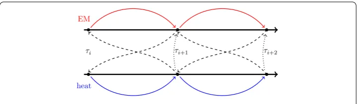
To simulate this model, () and () are solved successively. This can be repeated for one time step until convergence (see Algorithm ), similarly as done in Gauss-Seidel schemes. Here, we call it co-simulation. The scheme is also depicted in Figure . However, since convergence cannot be guaranteed for such schemes in general, a proof is given in Sec-tion ..

Algorithm Co-simulation with the frequency transient model, with discretized temper-atureTi, discretized magnetic vector potentialaiand timeti.

: Initialize model

: T(t)←T : i←

: whileti<tenddo : T_i+←Ti : l←

: whilel<  or not convergeddo : Solve () foral+_i+

: Solve () forTl+_i+

: l←l+ 

Figure 2 Frequency-transient co-simulation approach.

From Algorithm  it can be seen that time steps are chosen according to the time con-stant of the heat equation and only one (complex) linear system is solved per iteration for the curl-curl equation in frequency domain. Thus the time step size is independent of the excitation frequencyω. In contrast, a time domain solution would require many time steps per period π/ωand consequently the solution of a large number of real-valued lin-ear systems. This is the reason, why the model is very efficient for high frequencies since there is multirate behavior.

3.2 Convergence analysis

We first verify that the Maxwell operator is bounded:

Lemma Let the EM problem()be given with adequate BC,IV for a frequencyω>ω.

Then the inverse of the discrete Maxwell operator exists and is bounded

jωMσ(T) –ωMε+CMνC

–

≤C(ω) ()

for some frequency dependent upper bound C(ω)that is independent of the tempera-ture.

Proof Beforehand we introduce some abbreviations:

X:=ωMε–CMνC, Z:= –X+jωMσ. ()

Forω>ω for someω the matrixX=X(ω) is real, symmetric positive definite and

Mσ =Mσ(T) is real, diagonal, positive semi-definite. Then

Z= (–X+jωMσ) =X/

–I+jωX–/MσX–/

X/, ()

whereX/:=U/U–for an eigendecompositionX=UU–. Now letA:=X–/_M

σX–/, which is real and symmetric positive semi-definite. It follows that the eigenvalue decomposition isA=Q–Q, withQ= . Then

Z–=X–/(–I+jωA)–X–/

=X–/–Q–Q+jωQ–Q–X–/

Z–_≤X–/Q–_(–I+jω)–_QX–/

≤X–/··   +ω_λ

min

··X–/=X–=:C(ω),

becauseAis semidefinite.

The Lemma guarantees solvability of Maxwell’s equations independent of the tempera-ture. However, generalizations are possible but we focus here on the high frequency case because it exhibits a distinct multirate potential. In practice the time-harmonic approach can be used over a wide range of possible excitation frequencies. In particular for low-frequencies where the displacement currents are often disregarded [, ]. Furthermore for other choices of gauging similar results are found. Also in pure transient simulation [], a wide range of excitation frequencies is covered in practice.

Theorem Let the coupled problem()-()be given with adequate BC,IV for a frequency

ω>ω.We assume for nonlinear materials,e.g.,metals,positivity and differentiability for

σ(T)w.r.t.temperature T andσ< .Let the exact(monolithic)solution be denoted by_a∞ andT∞,then the iteration is convergent for hismall enough with

Tl+_–T∞_≤C(ω)h

iTl–T∞,

where C(ω)is uniformly bounded. Furthermore, we have C(ω) =O(_ω) for sufficiently

largeω.

Proof Consider the inner loop of Algorithm  (steps  and ). It consists of () and (). We prove convergence for this inner loop and use the same abbreviations as introduced in () with the shortcutZl_:=Z(Tl_{). Then we deduce from ()}

Zl_al+₌

j_s ⇔ _al+_=Zl–

j_s ()

due to the Lemma above. We defineN:=SM˜ kS˜, use () withT∞ anda∞ subtract it from ()

(Mρc+hiN)

Tl+–T∞=hi

ω

 P

Ml+_σ al+◦al+–M∞_σ a∞◦a∞

+hi

ω

PIm

j_s◦_al+_–a∞

. ()

Next, by adding and subtractinghiω  PM∞σ

al+◦al+, we have

(Mρc+hiN)

Tl+–T∞

=hi

ω

 P

Ml+_σ –M∞_{σ a}l+_◦al+

+hi

ω

 PM ∞ σ

al+◦_al+_–a∞_◦a∞

+hi

ω

PIm

j_s◦_al+_–a∞

Figure 3 Mimetic discretizations of Maxwell’s equations (e.g. by FIT) use a primal and dual grid.The discrete temperaturesTkare located at primary nodes, the

line-integrated electric field and the magnetic vector potentialsek=akare defined at primary edges and finally

the facet-integrated source current densityjkat dual

surfaces. The material laws relate the quantities on both grids, e.g., the conductivity connects by Ohm’s Law the currents and voltages, i.e.j_k=σk(Tk)ek. The figure shows

the case for a current inx-direction.

Now, let us consider the term

Ml+_σ –M∞_σ al+◦al+.

The conductivity matrixMσ is a diagonal matrix for any iteration step. We assume, that thekth componentσk(≤k≤n) depends only on the neighboring temperatureTk:= (PT)k, see Figure . Thus thekth component of the term can be written as

al+_k σk

T_kl+–σk

T_k∞al+_k .

Now the mean value theorem can be applied component-wise and yields for thekth com-ponent

al+_k σk

T_kl+–σk

T_k∞

al+_k =

al+_k σ_k(ζ)

al+_k T_kl+–T_k∞,

whereζkbetweenTkl+andTk∞, andσk is by assumption non-positive. Hence, in matrix vector notation with (ζ)k=ζk

Ml+_σ –M∞_{σ a}l+_◦al+_=A

l+Mσ(ζ)A

H

l+P

Tl+–T∞,

whereAl:=diag(al) and the diagonal matrixMσ(ζ) has only non-positive elements, i.e., it is negative semi-definite. It follows

LTl+–T∞=hi

ω

 PM ∞ σ

_al+_◦al+_–a∞_◦a∞

+hi

ω

PIm

j_s◦_al+_–a∞

()

with L:=Mρc +hiN–hiω 

PAl+Mσ(ζ)AHl+P whose inverse exists because it holds

L– _{≤ M}–

ρc, sinceMρc,Nare positive definite andMσ(ζ) is negative semi-definite. Multiplying () by the inverse of L, taking the norm and exploiting the upper bound

M–_ρcyields

Tl+_–T∞_≤M– ρc· hi

ω  PM

∞ σ

_al+_◦al+_–a∞_◦a∞

+hi

ω

PIm

j_s◦al+–a∞

. ()

Now, we need estimates for (a) the linear term_al+_–a∞

and (b) the quadratic term

_al+_◦al+_–a∞_◦a∞

(a) We start with the linear term: Consider()for the difference of exact solution and

(l+ )th iterate:

jωMl_σal+_–jωM∞ σ

a∞–X_al+_–a∞

= 

⇔ Z∞_al+_–a∞

+jωMl_σ–M∞_{σ a}l+_{= }

⇒ _al+_–a∞_≤ωZ∞–Ml

σ –M∞σ

al+ ()

≤ωZ∞–σ_max Tl–T∞Zl–j_s ()

≤C_(ω)ωσ_max Tl–T∞j_s ()

≤c(ω)Tl–T∞, ()

where we have exploited the Lemma to obtainc(ω) :=C

(ω)ω|σmax |

j_s. (b) We now consider the quadratic term in()

_al+_◦al+_–a∞_◦a∞

=_al+_–a∞

+_a∞_◦al+_–a∞

+_a∞

–_a∞_◦a∞

≤_al+_–a∞_◦al+_–a∞

+ _al+_–a∞_◦a∞

.

Becausea◦b ≤ ab, this can be written as

al+◦al+–a∞◦a∞≤al+–a∞+ al+–a∞a∞

≤c(ω)Tl–T∞+ c(ω)

a∞Tl–T∞, ()

where the Lemma gives us

_a∞

=Z∞–j_s≤C(ω)j_s. Using the estimates () and () in () gives

Tl+_–T∞_≤h i

ω

c(ω)PM –

ρcTl–T∞ωc(ω)M∞σ Tl–T∞ + ωC(ω)j_sM∞_σ +j_s.

Now consider the asymptotic behavior of this for largeωand smallhi. It holds

C(ω) =X–=ωMε–CMνC

–

∼ 

ω and

c(ω) =C_(ω)ωσ_max j_s ∼ 

ω.

Then, for fixedhiandωlarge enough, it follows that

Tl+–T∞≤hiC(ω)Tl–T∞,

3.3 Generalization

The frequency-transient model can be generalized in different ways. To enhance versatil-ity, one can use a multi-frequency excitation of the EM subsystem. An application would be steel hardening of gears [, ], where two frequencies are necessary to obtain a ho-mogeneous heating of the surface. Also to approximate periodic signals other than sinu-soidal, multi-frequency excitation can be used. This also allows for a Harmonic Balance approach, which enables usage of a nonlinear permeabilityμ.

.. Time dependent phasor

The model can be improved by weakening the assumptions made. In [] it is suggested to consider the complex phasor not as constant within one time window. This means () becomes

A(t) =  

_ˆ

Ac(T)ejωt+Aˆc(T)e–jωt=ReAˆc(T)ejωt. ()

Thus the derivatives are

∂A

∂t =Re

∂Aˆc

∂t ·e

jωt

+RejωAˆc·ejωt

, ()

∂_A

∂t =Re

∂_Aˆ c

∂t ·e jωt

+ Re

jω∂Aˆc ∂t ·e

jωt

–ReωAˆc·ejωt

, ()

whereAˆc:=Aˆc(T). Substituting ()-() into () yields

∇ ×μ–∇ × ˆAc

+ε

∂_Aˆ c

∂t + jω

∂Aˆc

∂t –ω

_Aˆ c

+σ(T)

∂Aˆc

∂t +jωAˆc

=ˆJsrc,

which is now a second order PDE with partial derivatives with respect to time as well. Note that in [] magnetoquasistatic formulation is used, so there the modification yields a first order system. However, since now both parts (EM and heat) have to be time integrated, the co-simulation of these can be called dynamic iteration [].

Due to the modification () changes to

˜ Q(T) =ω



 σ(T) ˆAc  c+

ω

 σIm

∂Aˆc

∂t · ˆAc

+Im(ˆJsrc· ˆAc)

+ 

∂Aˆc

∂t  c +Re ˆ Jsrc·

∂Aˆc

∂t

.

The convergence analysis can be extended accordingly.

.. MPDAE approach

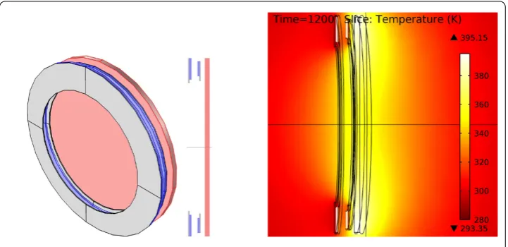
(a) d view and d cut view on geometry. From left to right: ferrite (gray), primary coil (blue), air, secondary coil (blue), ferrite (gray), air, steel slice (red). The left coil represents the charging station and the right coil the coil behind the number plate in the car.

(b) Temperature distribution after a simulation time of  min. The maximum temperature is . K. This is the cross section as shown in (a).

Figure 4 Model for an inductive charging system for electric vehicles (Comsol).

4 Frequency-transient co-simulation example

In this section the frequency-transient model is applied to an inductive charging system for electric vehicles. The charging system is modeled in a d-axisymmetric way by a pri-mary coil for the station and a secondary coil as receiver in the car. Both coils include ferrite. Additionally there is a steel slice to model the part of the car body behind the sec-ondary coil. The electric conductivity of this steel slice depends on the temperature, i.e., the system is mutually coupled. The geometry and simulation results are shown in Fig-ure . For more details of the set up we refer to [].

A constant conductivity would have lead to a single way coupled system and thus the magnetic vector potential would by a constant vector phasor. Models with a constant con-ductivity (according to the initial temperature) will systematically underestimate the heat-ing. In this case the obtained maximum temperature would be  K below the correspond-ing solution of the mutually coupled problem, [].

For mutually coupled problems the frequency-transient model has proved to be very efficient. This is expected, since the main part of the computational effort - the time in-tegration of the EM subsystem - is avoided. In this numerical exampleωwas chosen to be ·π· kHz. In fact the proposed co-simulation algorithm reached the end time of

tend=  min by using only  time steps withn≤ iterations (on averagen¯≈. it-erations). This coarse time grid sufficiently resolves the dynamics of the heat equation. For comparison, in a naive monolithic simulation with  time steps per period  mil-lion time steps would be necessary to resolve the dynamics of the EM subsystems. This underlines the computational gain.

5 Conclusions

con-vergence analysis is presented in detail. Concon-vergence for high frequencies is guaranteed. The error bound for the iteration decreases quadratically with higher frequencies. This re-sult also applies to approaches by Driesen and Hameyer [] and similar implementations in Comsol []. Thus the approach fits perfectly for applications where inductive heating either appears as losses or is intended.

Competing interests

The authors declare that they have no competing interests.

Authors’ contributions

All authors contributed to this paper as a whole. However, special merits go to DK and MR for sharing their experiences from industry, which led to the numerical example and introduction; to SS and MG for the work on the model; to CK, JtM and MK for their contribution to the analysis. All authors read and approved the final manuscript.

Author details

1_{Fachbereich Elektrotechnik und Informatik, Hochschule Bochum, Bochum, 44801, Germany.}2_{Lehrstuhl für Angewandte} Mathematik/Numerische Analysis, Bergische Universität Wuppertal, Wuppertal, 42119, Germany. 3_Technology Development and Qualification - Simulation, Leopold Kostal GmbH & Co. KG, Lüdenscheid, 58513, Germany.4_Graduate School of Computational Engineering, Technische Universität Darmstadt, Darmstadt, 64293, Germany.5_{Department of} Mathematics & Computer Science, TU Eindhoven, PostBox 513, MB Eindhoven, 5600, The Netherlands.

Acknowledgements

This work is supported by the German BMBF in the context of the SOFA project (grant number 03MS648E). The sixth author is supported by the ‘Excellence Initiative’ of the German Federal and State Governments and the Graduate School of Computational Engineering at Technische Universität Darmstadt.

Received: 23 April 2013 Accepted: 24 March 2014 Published: 3 June 2014

References

1. Schneider D:Wireless power at a distance is still far away [Electrons unplugged].IEEE Spectr2010,47(5):34-39. 2. Kaufmann C, Günther M, Klagges D, Richwin M, Schöps S, ter Maten EJW:Coupled heat-electromagnetic simulation

of inductive charging stations for electric vehicles. InProgress in Industrial Mathematics at ECMI 2012. Berlin: Springer; 2014. [Mathematics in Industry.]

3. Bartel A, Brunk M, Günther M, Schöps S:Dynamic iteration for coupled problems of electric circuits and distributed devices.SIAM J Sci Comput2013,35(2):B315-B335.

4. Driesen J, Hameyer K:The simulation of magnetic problems with combined fast and slow dynamics using a transient time-harmonic method.Eur Phys J Appl Phys2001,14:165-169.

5. Schöps S, De Gersem H, Weiland T:Winding functions in transient magnetoquasistatic field-circuit coupled simulations.Compel2013,32(6):2063-2083.

6. Haus HA, Melcher JR:Electromagnetic Fields and Energy. New York: Prentice Hall; 1989 [http://web.mit.edu/6.013_book/www/]

7. Clemens M, Gjonaj E, Pinder P, Weiland T:Numerical simulation of coupled transient thermal and electromagnetic fields with the finite integration method.IEEE Trans Magn2001,36(4):1448-1452.

8. Clemens M, Gjonaj E, Pinder P, Weiland T:Self-consistent simulations of transient heating effects in electrical devices using the finite integration technique.IEEE Trans Magn2001,37(5):3375-3379.

9. Weiland T:Time domain electromagnetic field computation with finite difference methods.Int J Numer Model

1996,9(4):295-319.

10. Bossavit A:Computational Electromagnetism: Variational Formulations, Complementarity, Edge Elements. San Diego: Academic Press; 1998 [http://tut.fi/~bossavit/#Books]

11. Hiptmair R, Ostrowski J, Quast R:Modelling and simulation of induction heating. Technical Report 149, SFB 382, University of Tübingen; 2000.

12. Alotto P, Freschi F, Repetto M:Multiphysics problems via the cell method: the role of Tonti diagrams.IEEE Trans Magn2010,46(8):2959-2962.

13. Hahne P, Weiland T:3D eddy current computation in the frequency domain regarding the displacement current.

IEEE Trans Magn1992,28(2):1801-1804.

14. Clemens M, Weiland T:Numerical algorithms for the FDiTD and FDFD simulation of slowly varying electromagnetic fields.Int J Numer ModelSpecial Issue ’Finite Difference Time Domain and Frequency Domain Methods’, Invited Paper 1999,12(1/2):3-22.

15. Chen Q, Schoenmaker W, Chen G, Jiang L, Wong N:A numerically efficient formulation for time-domain electromagnetic-semiconductor co-simulation for fast-transient systems.IEEE TCAD2013,32(5):802-806. 16. Rudnev V:Induction hardening of gears and critical components. Part I.Gear Technol2008,2008:58-63. 17. Rudnev V:Induction hardening of gears and critical components. Part II.Gear Technol2008,2008:47-53. 18. Brachtendorf HG, Welsch G, Laur R, Bunse-Gerstner A:Numerical steady state analysis of electronic circuits driven

by multi-tone signals.Electr Eng1996,79:103-112 [doi:10.1007/BF01232919]. 19. COMSOL Multiphysics:Command reference; 2007 [www.comsol.com]

doi:10.1186/2190-5983-4-1