Virtual sensor models for real-time applications

www.adv-radio-sci.net/14/31/2016/ doi:10.5194/ars-14-31-2016

© Author(s) 2016. CC Attribution 3.0 License.

Virtual sensor models for real-time applications

Nils Hirsenkorn1, Timo Hanke1,2, Andreas Rauch2, Bernhard Dehlink2, Ralph Rasshofer2, and Erwin Biebl1

1_{Technical University of Munich, Associate Professorship of Microwave Engineering, Munich, Germany} 2_{BMW AG, Munich, Germany}

Correspondence to:Nils Hirsenkorn ([email protected])

Received: 15 January 2016 – Revised: 21 April 2016 – Accepted: 20 May 2016 – Published: 28 September 2016

Abstract.Increased complexity and severity of future driver assistance systems demand extensive testing and validation. As supplement to road tests, driving simulations offer vari-ous benefits. For driver assistance functions the perception of the sensors is crucial. Therefore, sensors also have to be modeled. In this contribution, a statistical data-driven sensor-model, is described. The state-space based method is capable of modeling various types behavior. In this contribution, the modeling of the position estimation of an automotive radar system, including autocorrelations, is presented. For render-ing real-time capability, an efficient implementation is pre-sented.

1 Introduction

For showing whether fully automated driving is safer than human operation, a very large distance is necessary (see e.g. Maurer et al. (2015, pp. 451–458) for first estimations). As searching rare errors is a challenge, simulations might sup-port street tests. Being able to focus on the most crucial sce-narios might decrease the required distance for road testing. Moreover finding weaknesses of driver assistance systems in early stages of the development helps improving the quality of the end product.

To enable virtual testing, most driving simulators are ca-pable of modeling vehicle dynamics and rendering the en-vironment. Furthermore various efforts address the genera-tion of scenarios (Behrisch and Weber, 2015; Prialé Olivares et al., 2016; Gruyer et al., 2013). For advanced driver assis-tance systems (ADAS) the main input is the perception of the sensors. Therefore, implementing realistic sensor behavior is crucial for virtual ADAS development.

Approaches for simulating perception include Hardware-In-The-Loop (HiL) systems: for cameras HiL (Gans et al.,

2009) setups or Software-In-The-Loop rendering (Gruyer et al., 2012) are viable alternatives. However, distance mea-suring sensors remain challenging to simulate. HiL setups for radar enable the simulation of one or a small number of tar-gets (Heuel, 2015; Rohde&Schwarz, 2015). Difficulties par-ticularly regarding the simulation of different angles remain. Lidar HiL simulation is equally problematic. Even if a well suited HiL system for distance measuring sensors would ex-ist, the question, what values to simulate (e.g. which posi-tion), remains.

A further motivation of virtual testing and sensor models for driving simulators is presented in Hanke et al. (2015); Hirsenkorn et al. (2015); Bernsteiner et al. (2013, 2015) and Schubert et al. (2014).

Former statistical approaches mainly focused on simple parametric sensor models (Schubert et al., 2014; Bernsteiner et al., 2013, 2015; Rasshofer et al., 2005; Hanke et al., 2015). However, as shown in the subsequent section, non-parametric models present various benefits regarding real-ism, changes in dimensionality of the simulated quantities and generic applicability.

Whilst electromagnetic wave propagation simulation can yield accurate results, its computation might be too time-consuming some applications in ADAS development, even when neglecting real-time requirements.

2 Modeling

In this section a sensor model generated by real test drive measurements is shown. The approach was first introduced in Hirsenkorn et al. (2015). It is shortly summarized and then extended to further increase the fidelity. At the end of this section, the advantages and disadvantages compared to para-metric statistical models are presented.

In the context of probability density functions, capitalized variables are commonly denoted by random variables. Lower case letters indicate realizations of random variables. Func-tions marked by a hat indicate that they are an estimate (e.g. the result of an estimator). Variables marked by a tilde ∼

indicate that the quantity was measured by the sensor which should be modeled.

The task of a statistical sensor model is to estimate the probability density function (PDF) pˆZsim|Xsim of the simu-lated sensor-output Zsim given a state Xsim=xsim of the

simulation. During run-time the simulator draws a sample zsimfrom this PDF. Depending on the model, the PDF needs

to be calculated at run-time. 2.1 Theory

The basic idea is illustrated in two sentences: for each sim-ulated situation, recorded situations that are similar to this situation are identified. The simulated measurement should then be close to the recorded measurements in the identified situations.

For a vivid derivation and further explanations, refer to Hirsenkorn et al. (2015).

The conditional PDFpˆZsim|Xsim, introduced in the previ-ous section, can be transformed to a joint PDF using Bayes’ theorem

ˆ

p(zsim|Xsim=xsim)=

p(zsim,xsim)

p(xsim)

=p(zsim,xsim)

c . (1) Here p(xsim)=c can be interpreted as a normalization

constant to integrate to one. It is constant, sincexsimis a fixed

quantity, regarding the state of the simulator at a specific time step. For the estimation of the joint PDF, a non-parametric, kernel density estimation (KDE) approach is used. As the joint PDF is at least two-dimensional, a multivariate KDE has to be performed. For the estimation a set ofN tuples of recorded measurements{zmea,t,xmea,t}t=1:Nis used.

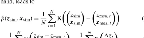
Adapt-ing the general definition (Hwang et al., 1994) to the case on hand, leads to

ˆ

p(zsim,xsim)=

1 N

N

X

t=1

K

zsim xsim

−

zmea,t

xmea,t

(2)

= 1

N

N

X

t=1

K

zsim−zmea,t

xsim−xmea,t

= 1

N

N

X

t=1

K

1zt

1xt

. (3)

In this equation the function K quantifies the equal-ity of the current vector of quantities in the simulation

(zT

sim,xTsim)T and the same quantities in recorded test drives

(zT_mea,t,xT_mea,t)T. However Sect. 2.2.2 will further discuss the function K.z describes quantities of the sensor, which should be modeled (e.g. a measured position of the target vehicle).x is a state which describes the influences on the quantities that should be modeled. An example forxmea,t is

the exact position of the target vehicle measured by a high precision reference system at step in timet. The stateszmea,t

andxmea,twere recorded at the same time.

A challenging task is the choice of proper combinations of quantities in the tuples. For example, the quantities included in the stateXshould contain as much information as possi-ble, to allow a precise prediction of its associated measure-mentZ. However, this would lead to a high dimensionality ofX. Considering the curse of dimensionality the state-space would become sparse. Sparse areas contain little information for the estimation ofpZsim|Xsim.

Parametric models share the problem of choosing a proper state description. Section 4 includes a proposal of supporting a reasonable choice of state variables.

2.2 Autocorrelated position modeling

In this section, an exemplary use of the modeling mentioned in the previous section is described. The task is a detailed modeling of the sensed position using an automotive radar system. It is assumed that only one unobstructed vehicle is being measured. However, this assumption can be dropped by splitting the model into multiple subtasks (Hanke et al., 2015).

2.2.1 Choice of the state description

As the state description (i.e. the state variables used in X orZ) is equal for the measurements and the simulation, the subscript indexes sim and mea can be dropped in this section. Figure 1 visualizes some of the used quantities.

The state variables of the sensor-outputz_t consist of the estimated target position(_eox,t,eoy,t)

T _{(e.g. of a radar system)}

relative to the true position of the closest corner of the vehi-cle(ox,corner,t, oy,corner,t)T. Summing up, the sensor output

is described by

zt=(eox,t−ox,corner,t,eoy,t−oy,corner,t)

T_{. (4)}

The index t denotes a discrete step in time (e.g. t∈1:N for the measurements or a certain step in time of the simu-lation). An exemplary state would bezT =(1[m],0.5[m])T.

The reason for makingzt relative to a point of the target

o corner,T

z T

Figure 1.Visualization of the state description.

Choosing the quantities of the influencesxt on the

sensor-output, depends on the effects which should be included. On one hand the true position of the closest corner of the tar-get vehicle is used (e.g. ox,corner,T =46 [m] in front of the

sensor andoy,corner,T =0.7 [m] to the left). As the estimated

target position is usually located at the observed side of the vehicle, choosing an unsuited position on the vehicle (e.g. the middle) would require a different model for each vehicle type (e.g. long trucks). Furthermore, the previous estimated target position, relative to the true position of the closest corner in the previous time stepzt−1, is used. This leads to

xt =(ox,corner,t, oy,corner,t,zTt−1)

T _=(oT t , zTt−1)

T_{. (5)}

In Hirsenkorn et al. (2015) we solely used the current true po-sition. Therefore no autocorrelation was implied. This led to big changes in the sensed position in subsequent time steps. However, as raw measurements are filtered, such jumps do not occur: even if the raw measurement jumps, it will be smoothed by a filter (e.g. a Kalman Filter, Venhovens and Naab, 1999; Bar-Shalom et al., 2004). Containing this infor-mation, the PDF in time stepT is located around the position of the measurement in the previous time stepT−1 . This can be observed in Fig. 3.

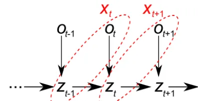
It should be remarked, that by including the previous mea-surement inxt, this process can be seen as a Markov-chain,

which is visualized in Fig. 2.

The tuples {zmea,t,xmea,t}t=1:N were recorded using an

automotive radar system (i.e. required for the measured tar-get position) and a high precision carrier phase, differential GPS including inertial measurement unit (i.e. required for the true corner positions). To obtain a reference for the relative position of the ego- and the target-vehicle, the high precision reference system is located in both vehicles.

2.2.2 Choice of the kernel function

The second degree of freedom in the application of the model is the selection of the kernel functionK. This function can be interpreted as a quantification of similarity. Various classes of kernel functions exist. As their statistical properties are sim-ilar, the choice should be based mainly on practical criteria (Simonoff, 2012). Due to the ease of computation and the common use in literature, the Gaussian kernel was selected. Moreover sampling from a Gaussian distribution can be im-plemented efficiently. The efficient implementation in Sect. 3

o

z

t

o

z

t+1

...

z

t-1

x

x

o

...

Figure 2.Depiction of the model as a Markov-chain.

benefits from this. A drawback of this kernel is the infinite support. However we neglect very low values, as their con-tribution to the resulting PDF is practically irrelevant. To ex-tend the kernel function to higher dimensionalities a product kernel is used (Simonoff, 2012), which leads to a Gaussian distribution with diagonal covariance matrix.

K(u)= 1

c0·

D

Y

d=1

Kd(ud);Kd=exp(

−u2_d

2·σ_d2) (6)

Dis the sum of the dimensionalities ofzandx.c0is a nor-malization constant.

It should be noticed, that choosing a Gaussian kernel does not imply the assumption of a Gaussian PDF, as the resulting PDF can be regarded as a weighted sum of multiple Gaus-sian PDFs. Because of the same reason, the independence of dimensions in the kernel does not imply independence of the dimensions in the resulting PDF.

Applying this kernel on the current example, leads to

K

1zt

1xt

= 1

c0Krel(1xt)·Kcon(1zt). (7)

Krel quantifies the relevance of a tuple using the difference

between the simulated state xsim and the tth

environment-statex_t. Choosing the variances properly is a trade-off: on one hand low variances assure the situation is as similar as possible. On the other hand this leads to a low number of tu-ples close to the simulated state. Equal to the curse of dimen-sionality, it would be hardly possible to estimate the PDF. To optimize this trade-off, the variances should decrease when the number of measurementsN increases. Furthermore the values depend on the unit of the dimension (e.g. variances need to be bigger using the unit mm than using m). The de-ployed kernel is

Krel(1xt)=exp(−

1xT_t 6−11xt

2 ); (8)

6= 

  

3 0 0 0

0 3 0 0

0 0 0.03 0

0 0 0 0.03



  

. (9)

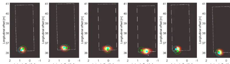
re-Figure 3.Course of the distribution of the PDF of the sensor-output in subsequent time steps. The sensor is located at the origin pointing in longitudinal direction. The white rectangle indicates the bounding box of the simulated target vehicle. The heat map shows the PDF

ˆ

p(z_sim|X_sim=x_sim). The green dot indicates the drawn position at the current time step. The cyan dot indicates the former sensor-output, maintaining the offset of the previous time step z_sim,t−1to the current closest corner. The white dots indicate the positions of recorded measurementszk. The size of each dot reveals the relevance of thekth tuple. For the shown plots, only∼5000 measurements, spread over

the whole field of view, were used.

garding the described influences. This choice can be inter-preted vividly as a difference in the true corner position of osim,T−omea,t=

√

3=1.73[m]leads to an equal notion of similarity as a difference in the last relative position output of zsim,T−1−zmea,t−1=

√

0.03=0.17[m]. HereT is the cur-rent step in time of the simulation and t is the index of a certain measurement. For the sake of completeness, the for-mer sentences are only valid if t−1 and t are subsequent steps in time of the same recording, and the time difference between two steps in time is equal in the simulation and in the measurements (e.g. 50 ms).

The second kernel function Kcon specifies the shape of

the contribution to the resulting PDF around the tth mea-sured sensor-output zt. Due to its simplicity, the variances

deployed inKconare computed using an automatic leave one

out cross-validation approach (Simonoff, 2012). Computing the variances can only be performed after knowledge of the current simulator statexsim,t (i.e. at run-time, in each time

step). The simple cross-validation is computationally expen-sive. To increase performance, the variances at several points ofXsimare computed before run-time and stored in a table.

Due to the smoothing ofKrelthe values are continuous. At

run-time, a table-lookup with interpolation is carried out. An alternative way of selecting the variances is using an automatic variance selection, for the relevance and the con-tribution at once. Result would be the same output variance in all areas. This would not account to different variances needed for different shapes of the PDFs in different areas of the state-space. For further information about variance se-lection (called bandwidth sese-lection in non-parametric liter-ature) and non-parametric statistics in general Scott (2015); Simonoff (2012) and Jiang (2010) can be consulted. 2.3 Critical discussion of the non-parametric model This section compares the introduced approach to classic, parametric models starting with the advantages, followed by the disadvantages.

Classical, parametric probability distributions are defined by a fixed amount of parameters. Often the parameters are adapted to fit the distribution to recorded measurements. However, the possible realism is limited since the distribution is restricted to a certain class Jiang (2010). Using real sensor data, the true underlying distribution will almost certainly not belong to the chosen class. Furthermore, the sensor behavior changes throughout the whole field of view. For example, in most cases the accuracy of a sensor is higher in the middle of the field of view than at the borders. For sensor models this implies, that the shape of the PDF differs depending on the position in the state-spaceXsim. In parametric sensor models

this is sometimes treated heuristically by a linear increasing standard deviation at the borders (Bernsteiner et al., 2013, 2015). The non-parametric model provides a more accurate adaption: the PDFpˆZsim|Xsim is calculated solely using mea-surements close to the current state of the simulationxsim,T

(i.e. measurements characteristic for the current state). Data-driven, non-parametric models are very flexible. An asymptotic view reveals this strength: with an infinite amount of data, a non-parametric model will converge almost sure to the true distribution (Wied and Weißbach, 2012). In contrast, parametric models lack this property.

The described model can also treat changes in dimension-ality ofzorx. This is of high practical relevance, for example when encountering object-losses. In non-parametric model-ing this can be included due to the separation into relevance and contribution. This article will not go into further detail here, however the next section and Hirsenkorn et al. (2015) will clarify this.

Furthermore, the behavior of the model at a certain time step can be linked to one tuple of a test drive. This means unexpected behavior in the simulation can be traced back to a specific measurement. The subsequent section will show this.

words, the model sticks too close to recorded measurements, shortcoming of generalization. Preventing overfitting comes at the cost of adding assertions on the behavior. As explained earlier in this section, the assumption of a specific distri-bution in parametric models destroys asymptotic properties. Moreover, overfitting is desirable in certain cases: the model sticks to real measurements but sacrifices completeness: be-havior, which has not been encountered, will not be modeled, but the model also will not add behavior that does not exist.

However, the authors also want to describe the drawbacks: the model is less interpretable and therefore hard to adapt to other behavior. Moreover, the modeling of a future sensor, of which no measurements are available yet, is barely possible. This is relevant for parallel development of ADAS and the sensor.

Another drawback is the dependence on sensor measure-ments including reference-measuremeasure-ments. This may be one of the main reasons, the approach has not been discussed earlier: accurate reference measurements were not avail-able. However, parametric models with parameters adapted to measurements share this drawback.

A big drawback of directly implementing the non-parametric approach is the high computational complexity. It increases with the number of measurements. Classical para-metric models, such as a Gaussian model, are of constant complexity. The implementation introduced in the subse-quent section further discusses this topic and provides a so-lution to minimize the drawback.

3 Computational improvements

This section investigates the computational complexity of the approach. Next solutions are presented to decrease the com-plexity to a fraction of the initial amount, whilst increasing the numerical accuracy.

Combining Eqs. (1), (3) and (7) leads to

ˆ

p(zsim|Xsim=xsim)=

1 N·c00

N

X

t=1

Krel(1xt)·Kcon(1zt)

(10)

= 1

N·c00

N

X

t=1

wt·Kcon(1zt). (11)

In practical use, the number of tuplesN may consist of 104 to 105measurements or more (i.e.∼1 h of test drive, consid-ering 20 Hz update frequency). This is why processing this equation needs to be highly optimized.

Since the relevance computationKrel(1xt), can be seen as

the inverse of a distance measure, large distances lead to neg-ligible values. Therefore, highly efficient standard algorithms of fixed radius near neighbors search (Muja and Lowe, 2009), to obtain the relevant samples, can be used. The solutions of-ten contain optimizations such as a graph construction at the

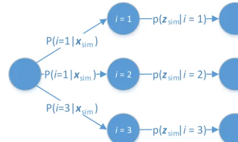
i = 2 i = 1

P(i=1|x )

P(i=1|x )

P(i=3|x )

p(z |i = 2)

p(z |i = 1)

sim

sim

sim

i = 3

p(z |i = 3)

sim

sim

Figure 4.The two stage drawing process.

beginning, which can be performed before run-time. After identifying the closest points, the more expensive relevance computation is performed only to the closest points – a small fraction of all samples. The remaining points are neglected for further computation since their relevance is practically zero. We use an R-tree (Beckmann et al., 1990) implementa-tion of the C++ library boost.

The direct way of drawing from Eq. (11) is the evaluation of the PDF at a lot of support points. Besides being com-putationally expensive, reconstructing the PDF using sup-port points is practically always a lossy approximation. Next the drawing has to be performed from the multidimensional complexly shaped PDF. This step also inefficient.

A more accurate and faster way of evaluating the PDF can be executed by a two stage drawing process. Following the law of total probability and comparing to Eq. (11) leads to

ˆ

p(zsim|Xsim=xsim)=

N

X

t=1

P (t|xsim)·p(zsim|t ) (12)

=

N

X

t=1

wt

N·c00·Kcon(1zt). (13)

At first, the tuple is selected which should be followed. This is done by a weighted drawing usingw1:N. Then drawing

samples from the Gaussian distributionKcon(1zt), located

at the sensor-outputztof the selected tuple, is executed.

Fig-ure 4 visualizes this process forN=3 measurements. Summing up, drawing values using this implementation is statistically equivalent to drawing using the original PDF. Furthermore this algorithm is missing the necessity of an ex-plicit representation of the PDF, which could only be approx-imated by support points. Therefore it is able to reconstruct the desired PDF more accurately than the direct evaluation.

It should be noted that this derivation also shows the pos-sibility to identify the originxt of a certain behavior in

Figure 5.The upper figure shows an analytically computed, binned relative frequency using an integration of Eq. (10). The lower figure presents a binned relative frequency using 95 000 samples drawn by the two stage drawing process described in Eq. (12).

3.1 Verification

Figure 5 compares an analytically computed, binned PDF (i.e. the PDF we actually want to draw from, Eq. 10), and the binned relative frequency resulting from 95 000 samples drawn using the two stage process (Eq. 12). The values of the borders of the bins are the same in both figures. This ensures the comparability and shows that the PDF is not shifted.

Besides the random fluctuations, which were to be ex-pected due to the random nature of the drawing process, both plots show good agreement. This result could be reproduced on arbitrary other PDFs, i.e. at other locations of the state-spaceXsimand other choices of the state-variables.

4 Conclusions and outlook

In this article a sensor model, simulating the position output was presented. The data-driven model was generated using real test drives including an automotive radar system in addi-tion to reference sensors. Whilst the scope of the effects reach from noise to field of view and object-losses, mainly autocor-relation of the sensed position was discussed. Next a critical discussion of the advantages and disadvantages, compared to classical parametric models, was presented. Furthermore an efficient implementation was derived, enabling real-time op-eration whilst achieving accurate results. The improvements were verified using an optical comparison.

Future works should focus on data-driven models, not us-ing high precision reference sensors but common sensors, which are available in production vehicles. This enhance-ment sets up test drives on any public road, leading to re-alistic scenarios. As production vehicles would contain the necessary equipment, this would also enable crowdsourc-ing of sensor models. The potential of fleet data regardcrowdsourc-ing various tasks in the automotive industry has already been shown in Ruhhammer et al. (2014), Klanner and Ruhham-mer (2015) and Protschky et al. (2015). This approach may not be possible for all quantities or microscopic effects, such as noise. However, macroscopic behavior, for instance the

field of view depending on weather conditions, might be ob-servable and quantifiable.

A quality criterion for quantifying the degree of realism would enable further improvements. Besides a well founded choice of the variances in the input kernel function, the the state representation could be optimized. For example, the se-lection of the state-representation could be automated. Fur-thermore, abstract state representations, acquired from di-mensionality reduction techniques, might boost the perfor-mance.

Acknowledgements. This work was funded by BMW Group. Special thanks to BMW Group for supplying the ego and the target vehicle including radar, lidar and reference sensors.

Edited by: R. Schuhmann

Reviewed by: two anonymous referees

References

Bar-Shalom, Y., Li, X. R., and Kirubarajan, T.: Estimation with ap-plications to tracking and navigation: theory algorithms and soft-ware, John Wiley & Sons, 2004.

Beckmann, N., Kriegel, H.-P., Schneider, R., and Seeger, B.: The R*-tree: an efficient and robust access method for points and rectangles, vol. 19, Proceedings of the 1990 ACM SIG-MOD international conference on Management of data, 322– 331, ACM New York, NY, USA©1990 ISBN:0-89791-365-5, doi:10.1145/93597.98741, 1990.

Behrisch, M. and Weber, M. (Eds.): Modeling Mobility with Open Data: 2nd SUMO Conference 2014 Berlin, Germany, 15–16 May 2014, Springer, 2015.

Bernsteiner, S., Magosi, Z., Lindvai-Soos, D., and Eichberger, A.: Phaenomenologisches Radarsensormodell zur Simula-tion laengsdynamisch regelnder Fahrerassistenzsysteme, VDI-Bericht 2169, Elektronik im Fahrzeug, 2013.

Bernsteiner, S., Magosi, Z., Lindvai-Soos, D., and Eichberger, A.: Radar Sensor Model for the Virtual Development Process, ATZelektronik worldwide, 10, 46–52, 2015.

Gans, N., Dixon, W., Lind, R., and Kurdila, A.: A hardware in the loop simulation platform for vision-based control of unmanned air vehicles, Mechatronics, 19, 1043–1056, 2009.

Gruyer, D., Grapinet, M., and De Souza, P.: Modeling and vali-dation of a new generic virtual optical sensor for ADAS pro-totyping, in: Intelligent Vehicles Symposium (IV), 969–974, doi:10.1109/IVS.2012.6232260, 2012.

Gruyer, D., Pechberti, S., and Glaser, S.: Development of full speed range ACC with SiVIC, a virtual platform for ADAS prototyp-ing, test and evaluation, in: Intelligent Vehicles Symposium (IV), 100–105, IEEE, 2013.

Hanke, T., Hirsenkorn, N., Dehlink, B., Rauch, A., Rasshofer, R., and Biebl, E.: Generic architecture for simulation of ADAS sen-sors, in: International Radar Symposium (IRS), 125–130, IEEE, 2015.

Hirsenkorn, N., Hanke, T., Rauch, A., Dehlink, B., Rasshofer, R., and Biebl, E.: A non-parametric approach for modeling sensor behavior, in: International Radar Symposium (IRS), 131–136, IEEE, 2015.

Hwang, J.-N., Lay, S.-R., and Lippman, A.: Nonparametric multi-variate density estimation: a comparative study, Signal Process., 42, 2795–2810, 1994.

Jiang, J.: Large sample techniques for statistics, Springer Science & Business Media, 2010.

Klanner, F. and Ruhhammer, C.: Backend Systems for ADAS, Springer, doi:10.1007/978-3-319-09840-1_29-1, 2015.

Maurer, M., Gerdes, J. C., Lenz, B., and Winner, H.: Autonomes Fahren. Technische, rechtlicht und geselschaftliche Aspekte, Springer-Verlag, doi:10.1007/978-3-662-45854-9, 2015. Muja, M. and Lowe, D. G.: Fast Approximate Nearest Neighbors

with Automatic Algorithm Configuration, International Confer-ence on Computer Vision Theory and Applications (VISAPP), 2, 2009.

Prialé Olivares, S., Rebernik, N., Eichberger, A., and Stadlober, E.: Virtual Stochastic Testing of Advanced Driver Assistance Sys-tems, in: Advanced Microsystems for Automotive Applications 2015, edited by: Schulze, T., Müller, B., and Meyer, G., Lec-ture Notes in Mobility, Springer International Publishing, 25–35, doi:10.1007/978-3-319-20855-8_3, 2016.

Protschky, V., Ruhhammer, C., and Feit, S.: Learning Traffic Light Parameters with Floating Car Data, in: Intelligent Transportation Systems (ITSC), 2438–2443, IEEE, 2015.

Rasshofer, R. H., Rank, J., and Zhang, G.: Generalized Modeling of Radar Sensors for Next-Generation Virtual Driver Assistance Function Prototyping, in: 12th World Congress on Intelligent Transport Systems, 2005.

Rohde&Schwarz: Measuring and testing with the ARTS9510 fam-ily of automotive radar target simulators – Application Bruchure, available at: http://www.rohde-schwarz.com (last access: Jan-uary 2016), 2015.

Ruhhammer, C., Hirsenkorn, N., Klanner, F., and Stiller, C.: Crowd-sourced intersection parameters: A generic approach for extrac-tion and confidence estimaextrac-tion, in: Intelligent Vehicles Sympo-sium, 581–587, IEEE, 2014.

Schubert, R., Mattern, N., and Bours, R.: Simulation von Sensor-fehlern zur Evaluierung von Fahrerassistenzsystemen, ATZelek-tronik, 9, 38–41, 2014.

Scott, D. W.: Multivariate density estimation: theory, practice, and visualization, John Wiley & Sons, 2015.

Simonoff, J. S.: Smoothing methods in statistics, Springer Science & Business Media, 2012.

Venhovens, P. J. T. and Naab, K.: Vehicle dynamics estimation using Kalman filters, Vehicle System Dynamics, 32, 171–184, 1999. Wied, D. and Weißbach, R.: Consistency of the kernel density