www.geosci-model-dev.net/9/2973/2016/ doi:10.5194/gmd-9-2973-2016
© Author(s) 2016. CC Attribution 3.0 License.
The Land Use Model Intercomparison Project (LUMIP)
contribution to CMIP6: rationale and experimental design
David M. Lawrence1, George C. Hurtt2, Almut Arneth3, Victor Brovkin4, Kate V. Calvin5, Andrew D. Jones6, Chris D. Jones7, Peter J. Lawrence1, Nathalie de Noblet-Ducoudré8, Julia Pongratz4, Sonia I. Seneviratne9, and Elena Shevliakova10
1National Center for Atmospheric Research, Boulder, CO, USA 2University of Maryland, College Park, MD, USA
3Karlsruhe Institute of Technology, Garmisch-Partenkirchen, Germany 4Max Planck Institute for Meteorology, Hamburg, Germany
5Joint Global Change Research Institute, College Park, MD, USA 6Lawrence Berkeley National Laboratory, Berkeley, CA, USA 7Met Office Hadley Centre, Exeter, UK
8Laboratoire des Sciences du Climat et de l’Environnement, Gif-sur-Yvette, France 9Institute for Atmospheric and Climate Science, ETH Zurich, Zurich, Switzerland 10NOAA/GFDL and Princeton University, Princeton, NJ, USA
Correspondence to:David M. Lawrence ([email protected])
Received: 4 April 2016 – Published in Geosci. Model Dev. Discuss.: 12 April 2016 Revised: 10 August 2016 – Accepted: 11 August 2016 – Published: 2 September 2016
Abstract. Human land-use activities have resulted in large changes to the Earth’s surface, with resulting implications for climate. In the future, land-use activities are likely to expand and intensify further to meet growing demands for food, fiber, and energy. The Land Use Model Intercompari-son Project (LUMIP) aims to further advance understanding of the impacts of land-use and land-cover change (LULCC) on climate, specifically addressing the following questions. (1) What are the effects of LULCC on climate and biogeo-chemical cycling (past–future)? (2) What are the impacts of land management on surface fluxes of carbon, water, and en-ergy, and are there regional land-management strategies with the promise to help mitigate climate change? In addressing these questions, LUMIP will also address a range of more detailed science questions to get at process-level attribution, uncertainty, data requirements, and other related issues in more depth and sophistication than possible in a multi-model context to date. There will be particular focus on the separa-tion and quantificasepara-tion of the effects on climate from LULCC relative to all forcings, separation of biogeochemical from biogeophysical effects of land use, the unique impacts of land-cover change vs. land-management change, modulation
of land-use impact on climate by land–atmosphere coupling strength, and the extent to which impacts of enhanced CO2 concentrations on plant photosynthesis are modulated by past and future land use.
po-tential for future land management decisions to aid in miti-gation of climate change. This paper documents these sim-ulations in detail, explains their rationale, outlines plans for analysis, and describes a new subgrid land-use tile data re-quest for selected variables (reporting model output data sep-arately for primary and secondary land, crops, pasture, and urban land-use types). It is essential that modeling groups participating in LUMIP adhere to the experimental design as closely as possible and clearly report how the model experi-ments were executed.
1 Introduction
Historic land-cover and land-use change has dramatically al-tered the character of the Earth’s surface, directly impacting climate and perturbing natural biogeochemical cycles. Land-use activities are expected to expand and/or intensify in the future to meet increasing human demands for food, fiber, and energy. From a broad perspective, the biogeophysical im-pacts of land-use and land-cover change (LULCC) on cli-mate are relatively well understood, with observational and modeling studies tending to agree that deforestation has led and will lead to cooling in high latitudes and warming in the tropics, with more uncertain changes in the mid-latitudes (e.g., Bonan, 2008; Davin and de Noblet-Ducoudré, 2010; Lee et al., 2011; Li et al., 2016; Pielke et al., 2011; Swann et al., 2012). The impact of land-cover change on, for ex-ample, global mean surface air temperature, has been and is projected to continue to be relatively small (Brovkin et al., 2013; Lawrence et al., 2012), but, regionally, climate change due to deforestation can be as large as or larger than that resulting from increases in greenhouse gas emissions (de Noblet-Ducoudré et al., 2012). Nonetheless, substantial dis-agreement exists across models in terms of their simulated regional climate response to LULCC (Kumar et al., 2013; Pitman et al., 2009), and some observed effects do not appear to be captured by models (Lejeune et al., 2016), contribut-ing to a lack of confidence in model projections of regional climate change. Variation among future scenarios of land-use change, which could depart significantly from historical trends due to large-scale adoption of either afforestation or biofuel policies, introduces another source of uncertainty that has not been examined in a systematic fashion (Jones et al., 2013b).
The biogeochemical impact of LULCC relates to emis-sions of greenhouse gases (GHGs) such as CO2, CH4, and N2O in response to LULCC (e.g., Canadell et al., 2007; Houghton, 2003; Pongratz et al., 2009; Shevliakova et al., 2009). Models estimate that the net LULCC carbon flux – the CO2exchange between vegetation and atmosphere due to LULCC such as emissions due to forest clearing and carbon uptake in regrowth of harvested forest – has accounted for ∼25 % of the historic increase in atmospheric carbon
diox-ide concentration (Ciais et al., 2014), but the LULCC flux remains one of the most uncertain terms in the global car-bon budget (Houghton et al., 2012). As on the biogeophysical side, models show a wide range of estimates for historic and future emissions due to LULCC (Arora and Boer, 2010; Boy-sen et al., 2014; Brovkin et al., 2013). When emissions of all GHG species due to LULCC are considered, the forcing due to LULCC accounts for∼45 % of the total historic (1850 to 2010) changes in radiative forcing (Ward et al., 2014).
as a tool for local or global climate mitigation (e.g., Canadell and Raupach, 2008; Marland et al., 2003).
Due to the predicted increases in global population and affluence as well as the increasing importance of bioenergy, demand for food and fiber is likely to surge during the com-ing decades. Expansion of active management into relatively untouched regions could satisfy a portion of the growing de-mand for food and fiber, but intensification is likely to play a stronger role in strategies for global sustainability (Foley et al., 2011; Reid et al., 2010). Therefore, we can antici-pate a growing contribution from land-management change to the overall impacts of LULCC on the climate system. The requirement of negative emissions to achieve low radiative forcing targets highlights the need for more comprehensive understanding of the impacts (e.g., on land use, water, nutri-ents, and albedo) and sustainability of carbon removal strate-gies such as bioenergy carbon capture and storage (BECCS, Smith et al., 2016).
Clearly, the impacts of land cover and land use on cli-mate are myriad and diverse and, while uncertain, are suf-ficiently large and complex to warrant an expanded activity focused on land use within CMIP6. The Land Use Model In-tercomparison Project (Lawrence et al., 2016, https://cmip. ucar.edu/lumip) addresses this topic in the context of CMIP6 (Eyring et al., 2016). The goal of LUMIP is to enable, co-ordinate, and ultimately address the most important science questions related to the effects of land use on climate. LU-MIP scientific priorities and model experiments have been developed in consultation with several existing model inter-comparison activities and research programs that focus on the role of land use in climate, including the Land-Use and Climate, IDentification of robust impacts project (LUCID, de Noblet-Ducoudré et al., 2012; Pitman et al., 2009), the Land-use change: assessing the net climate forcing, and op-tions for climate change mitigation and adaptation project (LUC4C, http://luc4c.eu/), the trends in net land carbon exchange project (TRENDY, http://dgvm.ceh.ac.uk/node/9), and the Global Soil Wetness Project (GSWP3). In addition, the LUMIP experimental design is complementary with and in some cases requires simulations from several other CMIP6 MIPs, including ScenarioMIP (O’Neill et al., 2016), C4MIP (Jones et al., 2016), LS3MIP (van den Hurk et al., 2016), DAMIP (Gillett et al., 2016), and RFMIP (Pincus et al., 2016). In all cases, the LUMIP experiments are complemen-tary and not duplicative with experiments requested in these other MIPs. We will reference these cross-MIP interactions throughout this paper, where applicable.
1.1 LUMIP activities
The main science questions that will be addressed by LUMIP in the context of CMIP6 are the following.
– What are the global and regional effects of land-use and land-cover change on climate and biogeochemical cy-cling (past–future)?
– What are the impacts of land management on surface fluxes of carbon, water, and energy?
– Are there regional land-use or land-management strate-gies with the promise to help mitigate climate change? In addressing these questions, LUMIP will also address a range of more detailed science questions to get at process-level attribution, uncertainty, data requirements, and other re-lated issues in more depth and sophistication than has been possible in a multi-model context to date. There will be particular focus on (1) the separation and quantification of the effects on climate from LULCC relative to all forcings, (2) separation of biogeochemical from biogeophysical ef-fects of land use, (3) the unique impacts of land-cover change vs. land-use change, (4) modulation of land-use impact on climate by land–atmosphere coupling strength, and (5) the extent to which the direct effects of higher CO2 concentra-tions on increases in global plant productivity are modulated by past and future land use.
Figure 1.Time series of global land area occupied by each LUH2 land-use state from 850 to 2015 (left). Note that extensions to 2100 for all
of the ScenarioMIP SSPs will also be provided. Fraction of each 0.25◦grid cell that is irrigated in year 2015 (top right). Fertilizer applied in
year 2015 (bottom right).
extent, constrains forest loss between the years 2000 and 2012 with Landsat-based forest loss data from Hansen et al. (2013), and uses a new historical wood harvest reconstruc-tion based on updated FAO data, new HYDE populareconstruc-tion data, and other sources. The LUH2 data set will include several new agricultural management layers such as gridded nitro-gen fertilizer usage based on Zhang et al. (2015), gridded ir-rigated areas (based on HYDE3.2), and gridded areas flooded for rice (also based on HYDE3.2), as well as the disaggrega-tion of wood harvest into fuel wood and industrial round-wood (i.e., timber that is cut for uses other than for fuel). Future scenarios (years 2016–2100) will also include biofuel management layers. To help address the issue of sensitivity to uncertainty in historical land-use forcing, two alternative historical land-use reconstructions have also been developed. These alternatives are based on same data sources, use the same algorithms, and are provided in the same format as the reference LUH2 product, but span a range of uncertainty in the key historical input data sets for agriculture and wood harvest. Specifically, the “high” reconstruction assumes high historical estimates for crop and pasture and wood harvest, and the “low” reference assumes low estimates for each of these terms, relative to the reference.
The LUH2 data set is available through the LUMIP web-site (https://cmip.ucar.edu/lumip) and will be described in a separate publication in this CMIP6 Special Issue. Guidance on use of the data will be provided in the LUH2 data set paper and through the LUMIP website.
Second, an efficient model experiment design, including both idealized and scenario-based cases, is defined that will enable isolation and quantification of land-use effects on cli-mate and the carbon cycle (see Sect. 2). The LUMIP exper-imental protocol enables integrated analysis of coupled and land-only (forced with observed meteorology) models that will support understanding and assessment of the forced re-sponse and climate feedbacks associated with land use and
the relationship of these responses with land and atmosphere model biases.
Third, a set of metrics and diagnostic protocols will be developed to quantify model performance, and related sen-sitivities, with respect to land use (see Sect. 3). De Noblet-Ducoudré et al. (2012) identified the lack of consistent eval-uation of a land model’s ability to represent a response to a perturbation such as land-use change as a key contribu-tor to the large spread in simulated land-cover change re-sponses seen in LUCID. As part of this activity, benchmark-ing data products will be identified to help constrain mod-els. Where applicable, these metrics will be incorporated into land model metrics packages such as the International Land Model Benchmarking (ILAMB, http://www.ilamb.org/) sys-tem.
1.2 Relevance of LUMIP to CMIP6 questions and WCRP Grand Challenges
Land-use change is an essential forcing of the Earth system, and as such LUMIP is directly relevant and necessary for CMIP6 Question (1) (Eyring et al., 2016): “How does the Earth System respond to forcing?”. LUMIP will also play a strong role in addressing the WCRP Grand Challenges (GC), particularly with respect to GC7 “determining how biogeo-chemical cycles and feedbacks control greenhouse gas con-centrations and climate change”, GC3 “understanding the factors that control water availability over land”, and GC4 “assessing climate extremes, what controls them, how they have changed in the past and how they might change in the future”. Due to the broad range of effects of land-use change and the major activities proposed, LUMIP is also of cross-cutting relevance to CMIP6 science questions (2) “What are the origins and consequences of systematic model biases?” and (3) “How can we assess future climate change given cli-mate variability, clicli-mate predictability, and uncertainties in scenarios?”.
1.3 Definitions of land cover, land use, and land management
Within LUMIP, we rely on prior definitions of land cover, land use, and land management (Lambin et al., 2006). Land cover refers to “the attributes of the Earth’s land surface and immediate subsurface, including biota, soil, topography, sur-face and groundwater, and human (mainly built-up) struc-tures”, and is represented in land models by categories like forest, grassland, cropland, or urban areas. Land use is the “purpose for which humans exploit the land cover”; e.g., a grassland may be left in its natural state, mowed, or uti-lized as rangeland for livestock. Land management refers to ways in which humans treat vegetation, soil, and water, and is captured in land models by processes such as irrigation, use of fertilizers and pesticides, crop species selection, or meth-ods of wood harvesting (selective logging vs. clear cutting). Thus, within the same land-cover category, several land uses can occur, and within the same land-use category, manage-ment practices can differ. Land-cover change usually goes hand in hand with land-use change, but the opposite is not true. Land-cover change can also be driven by natural pro-cesses such as a change in the biogeographic vegetation dis-tribution due to climate shifts or natural disturbance (Davies-Barnard et al., 2015; Schneck et al., 2013). For the purposes of LUMIP, the term “LULCC” includes anthropogenically driven land-cover change only.
2 Experimental design and description
In this section, we begin with a discussion and recommenda-tions on the specification of land use in CMIP6 Diagnostic, Evaluation and Characterization of Klima (DECK) and
his-torical experiments and other MIP experiments (Sect. 2.1). Also in this section, we outline the full set of requested LU-MIP experiments (Sects. 2.2 and 2.3). LULU-MIP includes a two-phase, tiered, model experiment plan. Phase one fea-tures a coupled model simulation with an idealized deforesta-tion scenario that is designed to advance process-level un-derstanding and to quantify model sensitivity to land-cover change impacts on climate and biogeochemical stocks and fluxes. Phase one also includes a factorial set of land-only model simulations that allow assessment of the forced re-sponse of land–atmosphere fluxes to land-cover change as well as examination of the impacts of various land-use and land-management practices. Phase two experiments will fo-cus on the quantification of the historic impact of land use and the potential for future land-management decisions to aid in the mitigation of climate change. A forum for discussion of the experiments and for distribution of minor updates to or clarifications of the experimental design will be hosted at the LUMIP website (https://cmip.ucar.edu/lumip).
Details of the model experiments are described below. The full set of LUMIP experiments includes
– Tier 1 (high priority): 500 years GCM/ESM; ∼650 years land-only; and
– Tier 2 (medium priority): 500 years GCM/ESM; up to 1500 to 3000 years land-only.
Note that these totals only represent the LUMIP-sponsored simulations. LUMIP analysis requires control simulations from other MIPs, e.g., a pre-industrial control DECK simu-lation or a CMIP6 historical simusimu-lation. We note the required “parent” simulation and responsible MIP, where applicable.
In Sects. 2.2 and 2.3, we describe each experiment in detail. Also included is the scientific rationale for the par-ticular experiment or set of experiments. The heading for each experiment includes several relevant pieces of infor-mation according to the following format – Short descrip-tion (CMIP6 experiment ID, model configuration, Tier X, # years) – where the model configuration is either land-only (offline land simulations forced with observed meteorology), GCM (fully coupled simulation, concentration-driven), or ESM (fully coupled simulation, emissions-driven).
2.1 Land-use treatment in the CMIP6 DECK,
historical experiments, and other MIP experiments There exists a large diversity in representation of LULCC among different land models, and therefore it is typically non-trivial to define what is meant by the terms “land use” and, in particular, the term “constant land use”. Several CMIP6 simulations both within LUMIP and in other CMIP6 MIPs require land use to be held constant in time, includ-ing (1) DECK experiments includinclud-ing CO2-concentration and CO2-emission driven pre-industrial control simulations (
1 % year−1CO2increase (1pctCO2) simulations, (2) LUMIP no land-use change simulations (Sect. 2.3.1), (3) C4MIP idealized simulations including biogeochemically coupled 1 % year−1CO2 increase (1pctCO2-bgc) and other C4MIP Tier 2 idealized simulations, and (4) ScenarioMIP extension simulations for the period 2100–2300 (ssp126-ext, ssp585-ext), for which land-use data will not be provided.
LUMIP provides the following recommendations to clar-ify treatment of constant land use. Land cover and land use should be fixed according to the LUH2 specifications for the constant land-use reference year (e.g., year 1850 for the DECK pre-industrial control simulation, year 2100 for Sce-narioMIP extension simulations). The fraction of cropland and pastureland, as well as the crop type distribution, should be held constant. Any land management (e.g., irrigation, fer-tilization) that exists for the constant land-use year should be maintained at the same level. Wood harvesting for timber and shifting cultivation, specified by the LUH2 land-use recon-structions (i.e., through transition matrices or the mass of har-vested wood), should be implemented if a model’s land-use component permits these processes to be maintained through time at a specified level. If the fire model utilizes population density or other anthropogenic forcings to determine fire ig-nition and/or suppression rates, then this forcing should also be held constant. We recognize that the diversity of model approaches means that the definition and requirements for constant land management may differ across models. Groups will need to make their own decisions with respect to the treatment of land management in constant land-use scenar-ios, for example with respect to specification of harvesting on croplands, grazing on pastureland, application of fertiliz-ers, level of irrigation, and wood harvest. Wood harvest, in particular, may require model-specific treatment since turn-ing off wood harvest in the ScenarioMIP 2100–2300 exten-sion runs is likely to result in unrealistic carbon stock trends, while maintaining wood harvest at year 2100 levels for an ad-ditional 200 years could unrealistically decimate the forests where the LUH2 data sets indicate wood harvest is happening in 2100. We stress that the individual modeling group deci-sions should be made within the context of achieving an equi-librated biogeophysical and biogeochemical (e.g., carbon, ni-trogen) land state for the pre-industrial 1850 control config-urations and to minimize any discontinuities in the shift be-tween a constant land-use simulation and a subsequent tran-sient land-use simulation (see the next paragraph for further clarification and discussion). Furthermore, the treatment of constant land use and land management should be clearly documented for each model and experiment. Because some land models are driven by annual maps of land use and others require transition rates between different land-use categories, LUMIP will provide two different 1850 constant land-use data sets – fraction of pastures and crops in 1850 and a one-time set of gross transitions from potential vegetation to the 1850 land-use state.
LUMIP acknowledges and endorses the need for flexi-ble strategies to initialize CMIP6 historical simulations and DECK AMIP simulations. This flexibility is necessitated by (1) considerable structural differences among CMIP6-participating land models, especially with respect to land use (e.g., models with and without wood harvest) and vegeta-tion dynamics (e.g., prescribed vs. prognostic vegetavegeta-tion type and age distributions), (2) different spinup strategies for land-only models vs. coupled GCMs and ESMs (e.g., spinup for potential vegetation vs. constant 1850 land use), and (3) un-certainties in PI-Control experiments due to omission of doc-umented secular multi-century trends in vegetation and soil carbon storage and land-use carbon emissions prior to 1850 (Pongratz et al., 2009; Sheviliakova et al., 2009). There are several strategies that have been used in the past and dis-cussed by the modeling groups at the present time, including – a “seamless” transition from the PI-control to historical
as suggested by Jones et al. (2016); and
– a “bridge” experiment from an equilibrated ESM spinup with potential vegetation and subsequent application of a land-use scenario applied at a year prior to 1850 (Sent-man et al., 2011; Shevliakova et al., 2013).
Consequently, LUMIP does not provide any recommen-dation on land initialization but requests that all model-ing groups document their initialization procedure for their CMIP6 historical simulations and report any differences in biogeophysical and biogeochemical land states between the 1850 pre-industrial control and the beginning of the CMIP6 historical simulations in 1851. As noted above, a forum for discussion along with additional recommendations and clar-ifications with respect to initialization, the configuration of “constant land use”, use of the LUH2 data, and other top-ics will be maintained through the LUMIP website (https: //cmip.ucar.edu/lumip).
2.2 Phase 1 experiments
Phase 1 consists of two sets of experiments: (a) an idealized coupled deforestation experiment that enables analysis of the biogeophysical and biogeochemical response to land-cover change and the associated changes in climate in a controlled and consistent set of simulations (Table 1) and (b) a series of offline land-only simulations to assess how the representation of land cover and land management affects the carbon, water, and energy cycle response to land-use change (Table 2). 2.2.1 Global deforestation (deforest-glob, GCM, Tier 1,
80 years)
Description: Idealized deforestation experiment in which
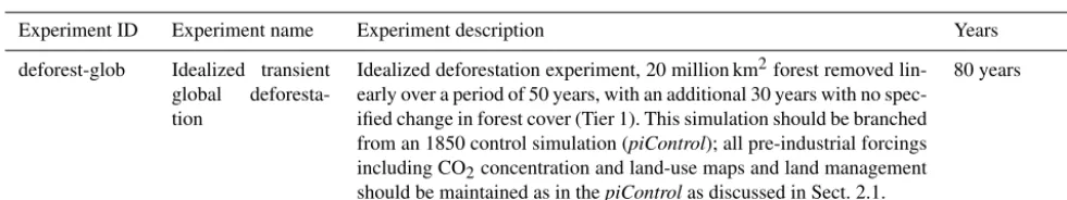
Table 1.Idealized deforestation experiment designed to gain process understanding and to assess biogeophysical role of land-cover change on climate and inter-compare modeled biogeochemical response to deforestation (concentration-driven).
Experiment ID Experiment name Experiment description Years
deforest-glob Idealized transient
global
deforesta-tion
Idealized deforestation experiment, 20 million km2forest removed
lin-early over a period of 50 years, with an additional 30 years with no spec-ified change in forest cover (Tier 1). This simulation should be branched
from an 1850 control simulation (piControl); all pre-industrial forcings
including CO2concentration and land-use maps and land management
should be maintained as in thepiControlas discussed in Sect. 2.1.
80 years
Figure 2.A schematic of the experimental setup in thedeforest-glob
experiment.(a)Scenario of forced changes in the global forest area.
(b)Sorting and selection of the grid cells that should be deforested.
(c)Transition of carbon pools after deforestation.
be branched from an 1850 control simulation (piControl); all pre-industrial forcings including CO2 concentration and land-use maps and land-management should be maintained as in the piControl and discussed in Sect. 2.1. The branch should occur at least 80 years prior to the end of the piControl simulation so thatdeforest-globandpiControlcan be directly compared. In order to concentrate the deforestation from grid cells with predominant forest cover, deforestation should be restricted to the top 30 % of land grid cells in terms of their area of tree cover. Effectively, this concentrates the defor-estation in the tropical rainforest and boreal forest regions (Fig. 3). To do this:
1. Sort land grid cells by forest area and select the top 30 % (gcdef, Fig. 2b).
2. Calculate tree plant type loss for each year at each grid cell by attributing the 400 000 km2year−1 forest loss proportionally to their forest cover fraction across the
gcdefgrid cells.
Step 2 is formalized as follows. Let f (x, y, t )be the forest fraction in grid cell (x, y)at the end of yeart (0≤t≤80);
A(x, y) is the area of the grid cell (million km2). At t= 0 (initialization of deforest-glob), forest fraction should be equal to that of year 1850 in the piControl. The total forest area, Ftot (million km2), within the grid cells identified for deforestation (gcdef) in Step 1 is
Ftot=
X
gcdef
f (x, y, t=0)A(x, y). (1)
IfFtotis more than 20 million km2, then the scaling coeffi-cientkgcdefis
kgcdef=
20
Ftot
≤1 (2)
and temporal development of forest fraction in deforested grid cells is calculated as follows:
f (x, y, t )=
(
f (x, y, t=0)(1−kgcdeft
50 ) 0< t≤50
f (x, y, t=0)(1−kgcdef) t >50
(3)
IfFtotis less than or equal to 20 million km2, then the scaling coefficientkcgefis taken as 1.
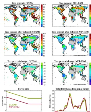
Trees should be replaced with natural unmanaged grass-lands. Land use and land management should be maintained at 1850 levels as in the piControl experiment. All above ground biomass (cWood, cLeaf, cMisc) should be removed and below ground biomass (cRoot) transferred to appropriate litter pools (Fig. 2c). If there is no separation of above and be-low ground biomass in the model, then the whole vegetation biomass pool (cVeg) should be removed. The replacement of forest with natural grasslands should be done in such a way that the carbon (and nitrogen if applicable) from the forested soil is maintained and allowed to evolve according to natural model processes. If initial forest cover in thegcdefgrid cells is less than 20 million km2 then should linearly remove all the forested area from thegcdefgrid cells over 50 years and report the total area of forest removed. Note that even with substantially different initial forest cover in CCSM4 vs. MPI-ESM-P (the examples shown in Fig. 3), the prescribed land-cover change is quite similar for both models when using this deforestation protocol and that modelling groups should strive to produce similar deforestation patterns.
Table 2.Land-only land-cover, land-use, and land-management change simulations. Assess relative impact of land-cover, land-use, and
land-management change on fluxes of water, energy, and carbon; forced with historical observed climate. The simulationsland-hist,
land-hist-altStartYear andland-noLuare Tier 1, all other simulations are Tier 2. All simulations should be pre-industrial to 2015, where the pre-industrial start can be either 1850 or 1700, depending on the model.
Experiment ID Description Notes
land-hist Same land model configuration, including
representa-tion of land cover, land use, and land management, as used in coupled CMIP6 historical simulation with all applicable land-use features active. Start year either 1850 or 1700 depending on standard practice for
par-ticular model. All forcings transient including CO2,
N-deposition, aerosol deposition, etc. Shared simula-tion with LS3MIP.
This simulation can and likely will be a different con-figuration across models due to different representa-tions of land use for each model. See the LS3MIP pro-tocol for full details, including details of the forcing data set and spinup.
land-hist-altStartYear Same asland-histexcept starting from either 1700 (for
models that typically start in 1850) or 1850 (for mod-els that typically start in 1700).
Comparison toland-histindicates impact of pre-1850
land-use change.
land-noLu Same as land-hist except no land-use change (see
Sect. 2.1 for explanation of no land use).
land-hist-altLu1 land-hist-altLu2
Same asland-histexcept with two alternative land-use
history reconstructions, that span uncertainty in
agri-culture and wood harvest. Specifically, thealtLu1is
a “high” reconstruction, assumes high historical
esti-mates for crop and pasture and wood harvest and
al-tLu2is a “low” reference assumes low estimates for
each of these terms, relative to the reference data set.
In combination withland-hist, allows assessment of
model sensitivity to different assumptions about land-use history reconstructions. Note that land land-use in 1700
and 1850 will be different to that inland-histso model
will need to be spun up again for both alternative data sets. Note that these reconstructions do not span the entire range of uncertainty, and the simulations should be considered sensitivity simulations.
land-cCO2 Same asland-histexcept with CO2held constant
land-cClim Same asland-histexcept with climate held constant Continue with spinup forcing looping over first
20 years of meteorological forcing data.
land-crop-grass Same asland-histbut with all new crop and
pasture-land treated as unmanaged grasspasture-land
For this simulation, treat cropland like natural grass-land without any crop management in terms of bio-physical properties but is treated as agricultural land for dynamic vegetation (i.e., no competition with nat-ural vegetation areas).
land-crop-noIrrigFert Same asland-histexcept with plants in cropland area
utilizing at least some form of crop management (e.g., planting and harvesting) rather than simulating crop-land vegetation as a natural grasscrop-land. . . Irrigated area and fertilizer area/use should be held constant.
Maintain 1850 irrigated area and fertilizer
area/amount and without any additional crop man-agement except planting and harvesting. Irrigation amounts with irrigated area allowed to change.
land-crop-noIrrig Same asland-histbut with irrigated area held at 1850
levels; only relevant ifland-histutilizes at least some
form of crop management (e.g., planting and harvest-ing)
Maintain 1850 irrigated area. Irrigation amounts within the 1850 irrigated area allowed to change
land-crop-noFert Same asland-histbut with fertilization rates and area
held at 1850 levels/distribution; only relevant if
land-histutilizes at least some form of crop management
(e.g., planting and harvesting)
land-noPasture Same asland-histbut with grazing and other
manage-ment on pastureland held at 1850 levels/distribution; i.e., all new pastureland is treated as unmanaged
Table 2.Continued.
Experiment ID Description Notes
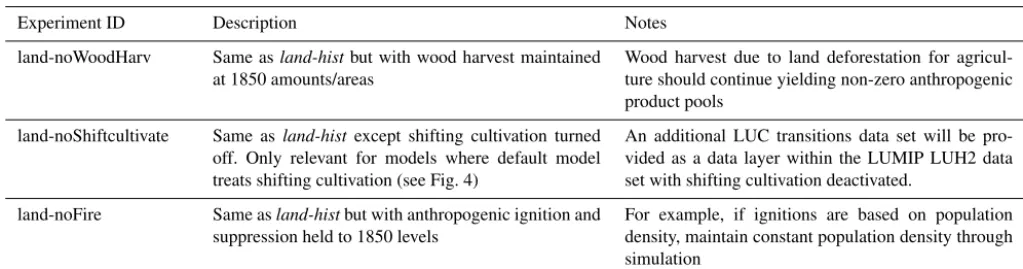
land-noWoodHarv Same asland-histbut with wood harvest maintained
at 1850 amounts/areas
Wood harvest due to land deforestation for agricul-ture should continue yielding non-zero anthropogenic product pools
land-noShiftcultivate Same asland-hist except shifting cultivation turned
off. Only relevant for models where default model treats shifting cultivation (see Fig. 4)
An additional LUC transitions data set will be pro-vided as a data layer within the LUMIP LUH2 data set with shifting cultivation deactivated.
land-noFire Same asland-histbut with anthropogenic ignition and
suppression held to 1850 levels
For example, if ignitions are based on population density, maintain constant population density through simulation
response to the climate change induced by deforestation is expected to be small over the 80-year simulation timescale.
We recognize that each participating land model has its own unique structures that may or may not be adequately covered in the above description sketched on the Fig. 2. Each modelling group should implement the deforestation in a manner that makes the most sense for their particular mod-elling system. It is important, however, that all groups strive to produce a spatial and latitudinal deforestation signal that replicates that shown in Fig. 3 as closely as possible. The goal of this experiment is to impose deforestation patterns that are as similar as possible across models so as to limit the impact of across-model differences in deforestation patterns on the multi-model evaluation of deforestation impacts on climate and carbon fluxes.
Rationale: this experiment is designed to be conceptually analogous to the 1 % year−1CO2 simulation in the DECK. Prior idealized global or regional deforestation simulations (Badger and Dirmeyer, 2015, 2016; Bala et al., 2007; Bathi-any et al., 2010; Davin and de Noblet-Ducoudré, 2010; Lorenz et al., 2016; Snyder, 2010) have proven informative and highlighted how both biogeophysical and biogeochemi-cal forcings due to land-use change contribute to temperature changes, how the ocean can modulate the response, and how remote effects of LULCC can be detected in some situations. However, differences in implementation of realistic historic or projected land-cover change across different models is a problem that has plagued prior land-cover change model in-tercomparison projects, with a third to a half – depending on season and variable – of the differences in climate response attributable to differences in imposed land cover (Boisier et al., 2012). The relatively simple LUMIP idealized deforesta-tion protocol will enhance uniformity in the prescribed de-forestation and therefore enable more direct and meaningful comparison of model responses to deforestation. The grad-ual deforestation allows a comparison across models with re-spect to what amplitude of forest loss is needed before a de-tectable signal emerges at the local and global level, and will provide insight into detection and attribution of land-cover change impacts at regional scales.
2.2.2 Land-only land-cover and land-use simulations (land-xxxx, land-only;land-hist,
land-hist-altStartYearandland-noLuare Tier 1, all others Tier 2, up to 13 simulations, 165 to 315 years each).
Description: a set of land-only simulations that are identi-cal to the LS3MIP (van den Hurk et al., 2016) historiidenti-cal land-only (land-hist; Table 2) simulation except with each simulation differing from theland-histsimulation in terms of the specific treatment of land use or land management, or in terms of prescribed climate. Note that all simulations should be forced with the default reanalysis data set provided through LS3MIP (GSWP3 at time of writing). The primary control experiment is land-hist; this is defined in LS3MIP. This experiment is required (Tier 1), even if the modeling group is not contributing to the full set of LS3MIP experi-ments. Theland-histsimulation should include land cover, land use, and land management that are identical to that used in the coupled CMIP6 historical simulation (see the next paragraph for more discussion). Two of the LUMIP simula-tions –land-hist-altStartYearandland-hist-noLu– are Tier 1. The remaining experiments are Tier 2. Detailed descriptions of the factorial set of simulations are listed in Table 2.
We anticipate that only a limited number of participating land models will be able to perform all the experiments, but the experimental design allows for models to submit the sub-set of experiments that are relevant for their model. In some instances, groups may also have a more advanced land model in terms of its representation of land-use-related processes than that which is used in the coupled CMIP6 historical sim-ulation. In these cases, we request that models submit the LUMIP Tier 1 land-only experiments with the configuration of the land model used in the coupled model CMIP6 histori-cal simulation, but groups are encouraged to provide an addi-tional set of land-only simulations with their more advanced model configuration.
Figure 3.Sample maps of fraction of grid cell covered by trees at the start of the idealized deforestation simulation, after idealized defor-estation (year 50), and the change in tree fraction by the end of the defordefor-estation period. Time series of forest area and zonal mean forest area loss are also shown. Examples are shown for two typical CMIP5 models with strongly differing initial forest cover. Even with the different initial forest cover, the deforestation patterns and amounts are broadly equivalent across the two models.
management affects the carbon, water, and energy cycle re-sponse to land-use change. This set of experiments utilizes state-of-the-art land-model developments that are planned across several contacted modeling centers and will contribute to the setting of priorities for land use for future CMIP activ-ities. The potential analyses that will be possible through this set of experiments are vast. We highlight several particular analysis foci here.
Theland-histandland-noLusimulations will provide
con-text for the global coupled CMIP6 historical simulations, en-abling the disentanglement of the LULCC forcing (changes in water, energy and carbon fluxes due to land-use change) from the response (changes in climate variables such as tem-perature and precipitation that are driven by LULCC-induced surface flux changes), though differences in the coupled model and observed climate forcing will need to be taken into account. The land-only simulations also allow more de-tailed quantification of the net LULCC flux.
Relative influence of various aspects of land management on the overall impact of land use on water, energy, and car-bon fluxes. For example, comparing theland-histexperiment to the experiment with no irrigation (land-crop-noirrig) will allow a multi-model assessment of whether or not the in-creasing use of irrigation during the 20th century is likely to have significantly altered trends of regional water and energy fluxes (and therefore climate) or crop yield/carbon storage in agricultural regions.
Pre-industrial land conversion for agriculture was sub-stantial (Pongratz et al., 2008) and has long-term and non-negligible legacy effects on the carbon cycle that last well beyond the standard 1850 starting year of CMIP6 histori-cal simulations (Pongratz and Caldeira, 2012). By comparing
land-histwithland-hist-altStartYearacross a range of
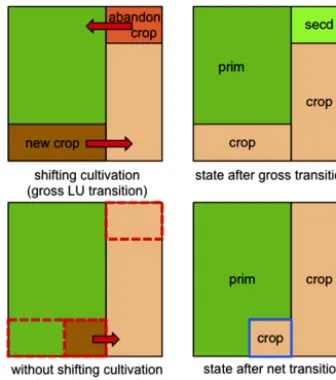
Figure 4. Schematic diagram showing difference between inclu-sion of shifting cultivation (gross transitions) vs. excluinclu-sion of shift-ing cultivation (net transitions). Where shiftshift-ing cultivation is in-cluded (upper row), new cropland (or pastureland) is taken (defor-estation) from primary land (“prim”) and abandoned to secondary land (“secd”) in parallel within a grid cell. In this case carbon fluxes, for example, are captured for each transition. Where shifting culti-vation is not represented (lower row), only the difference of new cropland minus abandoned cropland (represented by crop area out-lined in blue in bottom right figure) undergoes a transition to crop-land and no cropcrop-land is abandoned to form secondary crop-land. In this case, a smaller grid cell area fraction is affected by LUC. Adapted from Fig. 1 of Stocker et al. (2014).
Gross land-use transitions, especially due to shifting cul-tivation, can exceed net transitions by a factor of 2 or more (Hurtt et al., 2011). Accounting for gross transitions instead of just net transitions results in 15–40 % higher simulated net land-use carbon fluxes (Hansis et al., 2015; Stocker et al., 2014; Wilkenskjeld et al., 2014). For models that can represent shifting cultivation, a parallel experiment ( lnd-hist-noShiftcultivate) in which shifting cultivation is turned off (net transition) through an alternative set of provided land-use transitions will allow evaluation of the impact of shift-ing cultivation across a range of models and assumptions (Fig. 4).
Comparison of effects of LULCC on surface climate and carbon fluxes (which can be calculated by comparing historical and no-LULCC simulations) between the land-only simulations and the global coupled model simulations (Sect. 2.3.1) allows assessment of consequences of model climate biases on LULCC effects.
Uncertainty in the land-use history reconstruction is it-self a source of uncertainty in the impacts of historic LULCC. The alternative land-use history simulations ( land-hist-altLu1andland-hist-altLu2) in combination with the de-fault land-use history simulation (land-hist) provide
informa-tion on the sensitivity of the models to a range of plausible reconstructions of land-use history.
Impact of historic meteorological forcing data sets: it is critical to acknowledge that all observed historic forcing data sets are subject to considerable errors and uncertainty and that the weather and climate variability and trends repre-sented in these data sets may not accurately reflect reality, especially in remote regions where limited data went into ei-ther the underlying reanalysis or the gridded products. These limitations pose a challenge when comparing the model out-puts (like latent heat flux, for example) to observed esti-mates because biases may actually be a function of biases in the meteorological forcing data set rather than deficien-cies in the model. While the land-only LUMIP simulations will only be driven with a single atmospheric forcing data set (the reference data set used in theland-histexperiment of LS3MIP), the sensitivity of land model output to uncertainty in atmospheric forcing will be assessed in more depth within LS3MIP, which can inform the assessment of the land-only LUMIP simulations.
2.3 Phase 2 experiments
The Phase 2 LUMIP experiments are designed to pro-vide a multi-model quantification of the impact of historic LULCC on climate and carbon cycling and to assess the ex-tent to which land management could be utilized as a cli-mate change mitigation tool. This set of experiments in-cludes land-only and coupled historical and future simula-tions that are derivatives of historical or future simulasimula-tions within LS3MIP, ScenarioMIP, C4MIP as well as the CMIP6 Historical simulation with land use held constant or modified to an alternative land-use scenario (Table 3). These simula-tions will be used to assess the role of land use on climate from the perspective of both the biogeophysical and biogeo-chemical impacts and are likely to be of interest to DAMIP, C4MIP, ScenarioMIP, and LS3MIP.
2.3.1 Historical no land-use change experiment (hist-noLu; concentration-driven, Tier 1, 165 years)
Description: historical simulation that is identical to the
CMIP6 historical concentration-driven simulation, except that land use is held constant. All land use and management (irrigation, fertilization, wood harvest, gross transitions ceeding net transitions) is maintained at 1850 levels, in ex-actly the same way as done for the CMIP6 pre-industrial con-trol simulation (piControl).
Rationale: this simulation, when compared to the CMIP6
Table 3.Coupled Model Phase 2 simulations, all Tier 1.
Experiment ID Experiment name Experiment description Years
hist-noLu Historical with no
land-use change
Same as concentration-drivenCMIP6 historical(Tier 1) except with
LULCC held constant. See Sect. 2.1 for explanation of no land use. Two additional ensemble members requested in Tier 2.
1850–2014
ssp370-ssp126Lu
SSP3-7 with SSP1-2.6 land use
Same as ScenarioMIPssp370(SSP3-7 deforestation scenario, Tier 1)
except use land use from ssp126 (SSP1-2.6 afforestation scenario);
concentration-driven. Two additional ensemble members requested
(Tier 2) contingent on ScenarioMIPssp370large ensemble (Tier 2)
be-ing completed
2015–2100
ssp126-ssp370Lu
SSP1-2.6 with SSP3-7 land use
Same as ScenarioMIPssp126(SSP1-2.6 afforestation scenario, Tier 1)
except use land use from ssp370 (SSP3-7 deforestation scenario);
concentration-driven.
2015–2100
esm-ssp585-ssp126Lu
Emissions-driven SSP5-8.5 with SSP1-2.6 land use
Same as C4MIPesm-ssp585(Tier 1) except use SSP1-2.6 land use
(af-forestation scenario); emissions-driven
2015–2100
theCMIP6 historicalsimulation represents the integrated net LULCC flux. Note that the parallel set of land-only simula-tions (LS3MIPland-histexperiment and LUMIPland-noLu
experiment; see Sect. 2.1.3) will enable groups to disentangle the contributions of land-use change-induced effects on sur-face fluxes from atmospheric feedbacks and response (e.g., Chen and Dirmeyer, 2016), though the influence of differ-ences in land forcing in coupled vs. land-only simulations will need to be taken into account during the analysis. This experiment is directly relevant for detection and attribution studies (DAMIP).
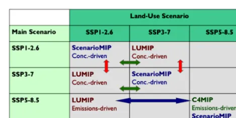
2.3.2 Future land-use policy sensitivity experiments (ssp370-ssp126Luandssp126-ssp370Lu, GCM concentration-driven, Tier 1, 2015–2100; esm-ssp585-ssp126Lu, ESM emission-driven, Tier 1, 2015–2100)
Description: these experiments are derivatives of
Scenari-oMIP (ssp370andssp126; see below for a short description of the Shared Socioeconomic Pathways (SSP) land-use sce-narios) and C4MIP (esm-ssp85) simulations (Fig. 5). In each case, the LUMIP experiment is identical to the “parent” sim-ulation, except that an alternative land-use data set is used. All other forcings are maintained from the parent simulation.
Rationale: both concentration-driven and emission-driven
LUMIP alternative land-use simulations are requested. Concentration-driven variants of ScenarioMIP ssp370 and
ssp126are required, but each uses the land-use scenario from the other: i.e., LUMIP simulationssp370-ssp126Luwill run with all forcings identical to ssp370, except for land use, which is to be taken fromssp126. These simulations permit analysis of the biogeophysical climate impacts of projected land use and enable preliminary assessment of land use and land management as a regional climate mitigation tool (green
Figure 5.Schematic describing the future land-use policy sensi-tivity experiments. Green arrows indicate set of experiments that permit analysis of the biogeophysical climate impacts of projected land use and enable assessment of land management as a regional climate mitigation tool. Red arrows indicate set of experiments that allow study of how the impact of land-use change differs at different
levels of climate change and at different levels of CO2
concentra-tion. Blue arrow indicates set of experiments that will enable quan-tification of the full effects of a different land-use scenario through both biophysical and biogeochemical processes. Brown arrows indi-cate set of experiments that allow quantification of the effects of the
climate-carbon cycle feedback on future CO2and climate change.
forc-ing level can be achieved by multiple socioeconomic scenar-ios with a negligible effect on the resulting climate (Van Vu-uren et al., 2014), an assumption that may not hold if pat-terns of land-use change associated with alternative SSPs di-verge significantly enough from one another (Jones et al., 2013b). Furthermore, including experiments in both low and medium/high radiative forcing scenarios allows examination of the extent to which the impact of land-use change differs at different levels of climate change and at different levels of CO2concentration (red arrows in Fig. 5). These sets of ex-periments can be utilized to provide partial guidance on the utility of careful land management as a climate mitigation strategy (Canadell and Raupach, 2008; Marland et al., 2003). Emission-driven simulations allow assessment of the full feedback (biogeophysical+biogeochemical) due to land-use change onto climate. In these simulations the ESMs sim-ulate the concentration of atmospheric CO2 in response to prescribed boundary conditions of anthropogenic emis-sions. Biogeophysical effects operate in the same way as in concentration-driven simulations but, in addition, the carbon released or absorbed due to land-use change will affect how the CO2 concentration of the atmosphere evolves in time. Additionally, emission-driven simulations permit assessment of consistency between Integrated Assessment Model predic-tions (which typically include the biogeochemical effect of land use as a carbon source but neglect the biophysical ef-fects) about land use and land-use change carbon fluxes with ESM modeled land-use emissions. C4MIP has requested an emission-driven variant tossp585, which will be performed in concentration-driven mode for ScenarioMIP. This will al-low quantification of the effects of the climate-carbon cycle feedback on future CO2 and climate change (brown arrow in Fig. 5). In LUMIP we request a further SSP5-8.5 simula-tion: emission-driven but with land use taken from SSP1-2.6. This experiment (esm-ssp585-ssp126Lu)will therefore par-allel the C4MIP emission-driven experiment (esm-ssp585)
but will allow us to quantify the full effects of a different land-use scenario through both biophysical and biogeochem-ical processes (blue arrow in Fig. 5).
Land-use scenarios in SSPs: the scenarios chosen for use
in CMIP6 were developed as part of the Shared Socioeco-nomic Pathways (SSPs) effort (Van Vuuren et al., 2014). Five SSPs were designed to span a range of challenges to mitiga-tion and challenges to adaptamitiga-tion. These SSPs can be com-bined with RCPs to provide a set of scenarios that span a range of socioeconomic assumptions and radiative forcing levels (Riahi et al., 2016). ScenarioMIP selected eight sce-narios from this suite for use in CMIP6. Within LUMIP, we focus on three of these scenarios in our experimental design, chosen because they span a range of future land-use pro-jections. The SSP5-8.5 is a high radiative forcing scenario, reaching 8.5 W m−2 in 2100, with relatively little land-use change over the coming century. The increase in radiative forcing is driven by increased use of fossil fuels; however, the combination of a relatively small population and high
agricultural yields leads to little expansion of cropland area (Kriegler et al., 2016). In contrast, the SSP3-7 is a world with a large population and limited technological progress, resulting in expanded cropland area (Fujimori et al., 2016). In the SSP1-2.6, efforts are made to limit radiative forcing to 2.6 W m−2. These mitigation efforts include reduced defor-estation as well as refordefor-estation and affordefor-estation, leading to a scenario where forest cover increases over the coming cen-tury (Van Vuuren et al., 2016). Figure 6 shows global time series of forest area, cropland area, pastureland area, wood harvest, area equipped for irrigation, and nitrogen fertiliza-tion amounts in the SSP scenarios, highlighting those sce-narios selected by ScenarioMIP and LUMIP.
3 Land-use metrics and analysis plans 3.1 Land-use metrics
A goal of LUMIP is to establish a useful set of model di-agnostics that enable a systematic assessment of land use– climate feedbacks and improved attribution of the roles of both land and atmosphere in terms of generating these feed-backs. The need for more systematic assessment of the ter-restrial and atmospheric response to land-cover change is one of the major conclusions of the LUCID studies. Boisier et al. (2012) and de Noblet-Ducoudré et al. (2012) argue that the different land use–climate relationships displayed across the LUCID models highlight the need to improve diagnos-tics and metrics for land surface model evaluation in general and the simulated response to LULCC in particular. These sentiments are consistent with recent efforts to improve and systematize land model assessment (e.g., Abramowitz, 2012; Best et al., 2015; Kumar et al., 2012; Luo et al., 2012; Ran-derson et al., 2009). LUMIP will promote a coordinated ef-fort to develop biogeophysical and biogeochemical metrics of model performance with respect to land-use change that will help constrain model dynamics. These efforts dovetail with expanding emphasis in CMIP6 on model performance metrics. Several recent studies have utilized various method-ologies to infer observationally based historical change in land surface variables impacted by LULCC or divergences in surface response between different land-cover types (Boisier et al., 2013, 2014; Lee et al., 2011; Lejeune et al., 2016; Li et al., 2015; Teuling et al., 2010; Williams et al., 2012).
● ● ● ● ● ● ● ● ● ● 34 36 38 40 42
2025 2050 2075 2100 Year Million km 2 SCENARIO ● SSP1−26 SSP2−45 SSP3−70 SSP4−34 SSP4−60 SSP5−85
(a) Forest area
● ● ● ● ● ● ● ● ● ● 24 26 28 30 32 34 36
2025 2050 2075 2100 Year Million k m 2 SCENARIO ● SSP1−26 SSP2−45 SSP3−70 SSP4−34 SSP4−60 SSP5−85
(c) Pastureland area
● ● ● ● ● ● ● ● ● ● 800 1200 1600
2025 2050 2075 2100 Year
Million tC yr
SCENARIO ● SSP1−26 SSP2−45 SSP3−70 SSP4−34 SSP4−60
(e) Wood harvest
● ● ● ● ● ● ● ● ● ● 16 18 20 22 24 26 28
2025 2050 2075 2100 Year Million km 2 SCENARIO ● SSP1−26 SSP2−45 SSP3−70 SSP4−34 SSP4−60 SSP5−85
(b) Cropland area
● ● ● ● ● ● ● ● ● ●
2 4
2025 2050 2075 2100 Year Million km 2 SCENARIO ● SSP1−26 SSP2−45 SSP4−34 SSP4−60 SSP5−85
(d) Irrigated cropland area
● ● ● ● ● ● ● ● ● ● 100 125 150 175 200
2025 2050 2075 2100 Year TgN yr SCENARIO ● SSP1−26 SSP2−45 SSP4−34 SSP4−60 SSP5−85
(f) Nitrogen fertilizer use
-1
-1
Figure 6.Global time series of land cover(a), land use(b, c, e), and land management(d, f)for the future simulations. Lines indicate SSP-RCP scenarios chosen for ScenarioMIP, with colored lines representing scenarios with specific LUMIP experiments. Data is provided by the IAM community. Data will be harmonized to ensure consistency between the end of the historical period and the beginning of the projection period for each of the scenarios. Note that not all IAMs predict all the LUH2 land management quantities (e.g., wood harvest is missing for SSP5-8.5). The missing land management variables will be generated during the harmonization process in a manner that is consistent with the underlying scenario.
LUMIP also proposes to develop a set of analysis metrics that succinctly quantify a model response to land use across a range of spatial scales and temporal scales that can then be used to quantitatively compare model response across differ-ent models, regions, and land-managemdiffer-ent scenarios. For a given variable, say surface air temperature, diagnostic calcu-lations will be completed for a pair of simucalcu-lations (offline or coupled) with and without land-use change. Across a range of spatial scales, spanning from a single grid cell up to re-gional, continental, and global, seasonal mean differences between control and land-use change simulations will be ex-amined. Differences will be expressed, for example, both in terms of seasonal mean differences and in terms of signal to noise (where “noise” refers to the natural interannual climate variability simulated in the model). Lorenz et al. (2016) em-phasize the importance of testing for field significance, espe-cially in the context of evaluating the statistical significance of remote responses to LULCC.
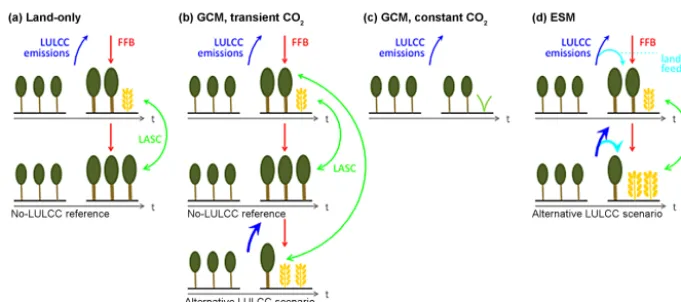
3.2 Net LULCC carbon flux: loss of additional sink capacity and the net land-use feedback
in-crease (Gerber et al., 2013; Mahowald et al., 2016; Pongratz et al., 2014). The land-use carbon feedback can be assessed in emission-driven simulations where LULCC carbon fluxes alter the atmospheric CO2 concentration and the land-use changes also affect the climate through biogeophysical re-sponses, both of which can then feed back onto the produc-tivity of both natural and managed vegetation. Over the his-torical period, a substantial fraction of the LULCC emissions have been offset with increased vegetation growth. Calculat-ing the net LULCC flux by differencCalculat-ing carbon stocks from a pair of simulations with and without LULCC will lead to net LULCC flux estimates that are about 20–50 % lower when calculated from a pair of emission-driven simulations (which include the land use–carbon feedback) compared to a pair of land-only simulations (Pongratz et al., 2014; Stocker and Joos, 2015).
Within LUMIP, several different model configurations are used that include the LASC and the land use–carbon feed-back to different extents (Fig. 7). Note that to isolate the effect of LULCC emissions from those of fossil-fuel emis-sions, a reference simulation is needed, which may be a no-LULCC simulation or a simulation with an alternative LULCC scenario. In the case of the idealized deforesta-tion experiments, where CO2 is kept constant over time, all changes in carbon stocks can be directly attributed to LULCC. The net LULCC flux, as quantified from the land-only simulation, will differ slightly from that calculated in GCM simulations since the GCM simulations include bio-geophysical climate feedbacks from LULCC. The difference in net LULCC flux between two LULCC scenarios as de-rived from the ESM setup follows a different definition, as the land-use carbon feedback is included and its effects can-cel only partly by difference of the two simulations.
3.3 Radiative forcing
A recognized limitation within CMIP5 was the difficulty in diagnosis of the radiative forcing due to different forcing mechanisms such as well-mixed GHGs, aerosols or land-use change. In addition, the regionally concentrated nature of biophysical land-use forcing limits the insight gained from quantifying it in terms of a global mean metric (or more strictly the effective radiative forcing, ERF; Davin et al., 2007; Jones et al., 2013a; Myhre et al., 2013). Experiments were performed within CMIP5 to explore different model re-sponses to individual forcings but were not designed to dis-tinguish how each forcing led to a radiative forcing of the climate system vs. how the climate system responded to that forcing. For CMIP6, RFMIP is designed to address this gap by including a factorial set of atmosphere-only simulations to diagnose the ERF due to each forcing mechanism individ-ually. Andrews et al. (2016) performed the Radiative Forcing MIP (RFMIP) land-use experiment to diagnose the histori-cal ERF from land use in HadGEM2-ES and found a forc-ing of −0.4 W m−2 or about 17 % of the total present-day
anthropogenic radiative forcing. Other studies indicate that the combined radiative forcing effect of land-use change may be as large as∼40 % of total present-day anthropogenic ra-diative forcing, when accounting for emissions of all GHG species due to LULCC (Ward et al., 2014). LUMIP will ben-efit from groups performing the RFMIP land-use experiment in addition to the LUMIP simulations.
3.4 Modulation of the land-use change signal by land–atmosphere coupling strength
An axis of analysis that has not been investigated in great detail is how a particular model’s regional land–atmosphere coupling strength signature (Guo et al., 2006; Koster et al., 2004; Seneviratne et al., 2010, 2013) affects simulations of the climate impact of land-use change. One can hypothe-size that LULCC in a region where the land is tightly cou-pled to the atmosphere, generally due to the presence of a soil moisture-limited evapotranspiration regime (Koster et al., 2004; Seneviratne et al., 2010), will result in a stronger climate response than the same LULCC in a region where the atmosphere is not sensitive to land conditions. In a sin-gle model study of Amazonian deforestation, Lorenz and Pit-man (2014) find that this is indeed the case – small amounts of deforestation in a part of the Amazon domain where the model simulates strong land–atmosphere coupling has a larger impact on temperature than extensive deforestation in a weakly coupled region. Similarly, Hirsch et al. (2015) show that different planetary boundary layer schemes, which lead to different land–atmosphere coupling strengths, can modulate the impact of land-use change on regional cli-mate extremes. LUMIP will collaborate with LS3MIP to sys-tematically investigate the inter-relationships between land– atmosphere coupling strength, which can be diagnosed in any coupled simulation (e.g., Dirmeyer et al., 2014; Seneviratne et al., 2010), and LULCC impacts on climate, and estab-lish to what extent differences in land–atmosphere coupling strength across models (Koster et al., 2004) contribute to dif-ferences in modeled LULCC impacts.
3.5 Extremes
Figure 7. Illustration of the different setups used in the LUMIP experiments, using the example of forest replacement by cropland or grassland. The loss of additional sink capacity (LASC) is a factor when environmental conditions change transiently, which is the case
when historical CO2concentrations, which implicitly include increases in CO2due to fossil-fuel burning (FFB) and LULCC, are prescribed
from observations. Prognostic LULCC emissions are directly “seen” by the terrestrial vegetation (natural and anthropogenic) only in the
ESM setup, where CO2 is interactive. In this case, a fraction of the LULCC emissions is taken up again by the vegetation (“land-use
carbon feedback”). Note that only atmospheric CO2is prescribed in(a–c), while other environmental conditions feed back with LULCC’s
biogeophysical effects.
of changes in albedo (Davin et al., 2014) and accumulated changes in soil moisture content (Wilhelm et al., 2015). Caful assessment will be necessary to validate the inferred re-lationships between LULCC and extremes, given partly con-tradicting results with respect to the effects of LULCC on climate extremes in models and observations (Lejeune et al., 2016; Teuling et al., 2010).
4 Subgrid data reporting
To address challenges of analyzing effects of LULCC on the physical and biogeochemical state of land and its interactions with the atmosphere (e.g., analyses proposed in Sects. 3.2– 3.5), LUMIP is including a Tier 1 data request of sub-grid information for four sub-grid categories(i.e., tiles) to per-mit more detailed analysis of land-use-induced surface het-erogeneity. The rationale for this request is that relevant and interesting sub-grid-scale data that represent the heterogene-ity of the land surface are available from current land mod-els but are not being used since sub-grid-scale quantities are typically averaged to grid cell means prior to delivery to the CMIP database. Several recent studies have demonstrated that valuable insight can be gained through analysis of grid information. For example, Fischer et al. (2012) used sub-grid output to show that not only is heat stress higher in ur-ban areas compared to rural areas in the present-day climate, but also that heat stress is projected to increase more rapidly in urban areas under climate change. Malyshev et al. (2015) found a much stronger signature of the climate impact of LULCC at the subgrid level (i.e., comparing simulated sur-face temperatures across different land-use tiles within a grid cell) than is apparent at the grid cell level. Subgrid
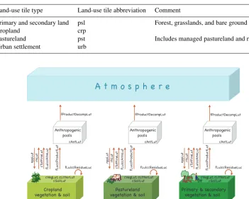
analy-sis can also lead to improved understanding of how models operate. For example, Schultz et al. (2016) showed, through subgrid analysis of the Community Land Model, that the as-sumption that plants share a soil column and therefore com-pete for water and nutrients has the side-effect of an effec-tive soil heat transfer between vegetation types that can alias into individual vegetation-type surface fluxes. Furthermore, reporting carbon pools and fluxes by tiles will enable assess-ment of land-use carbon fluxes not only with the standard method of looking at differences between land-use and no land-use experiments (e.g., as described in Sect. 3.2), but also within a single land-use experiment, utilizing bookkeeping approaches (Houghton et al., 2012) that allow a more direct comparison of observed and modeled carbon inventories. 4.1 Types of land-use tiles
Table 4.Land-use tile types and abbreviations.
Land-use tile type Land-use tile abbreviation Comment
Primary and secondary land psl Forest, grasslands, and bare ground
Cropland crp
Pastureland pst Includes managed pastureland and rangeland
Urban settlement urb
A t m o s p h e r e
Anthropogenic pools
Cropland
vegetation & soil Pasturelandvegetation & soil Primary & secondary vegetation & soil
nppLu
t
rhLu
t
cT
otF
ireLu
t
fLu
lccA
tmLu
t
fLuc
cP
ro
duc
tLu
t
fLulccResidueLuc fLulccResidueLuc fLulccResidueLuc
cVegLut,cLitterLut cSoilLut
cAntLut
cVegLut,cLitterLut
cSoilLut cVegLut,cSoilLutcLitterLut
Anthropogenic pools
nppLu
t
rhLu
t
cT
otF
ireLu
t
fLu
lccA
tmLu
t
fLuc
cP
ro
duc
tLu
t cAntLut
Anthropogenic pools
nppLu
t
rhLu
t
cT
otF
ireLu
t
fLu
lccA
tmLu
t
fLuc
cP
ro
duc
tLu
t cAntLut
fProductDecompLut
fProductDecompLut fProductDecompLut
Figure 8.Exchanges and transfers affecting storage of biogeochemical constituents in land models under LULCC. Variable descriptions can be found in Table 5. Urban tile not shown, but if carbon fluxes are calculated on a particular model’s urban tile, then these fluxes should be reported for the rban tile as well.
4.2 Requested variables and rules for reporting Overall, there are five classes of variables that are requested. These variables describe (a) the subgrid structure and how it evolves through time, (b) biogeochemical fluxes, (c) biogeo-physical variables, (d) LULCC fluxes and carbon transfers (Fig. 8), and (e) carbon stocks on land-use tiles. A list of re-quested land-use tile variables is shown in Table 5. However, this list is subject to change. Modelers should refer to the CMIP6 output request documents for the final variable list.
Subgrid tile variables should be submitted according to the following structure, using leaf area index (LAI) as an exam-ple: laiLut (lon, lat, time, landusetype4) – where the landuse-type4 dimension has an explicit order of psl, crp, pst, and urb, where “psl” is primary and secondary land, “crp” is cropland, “pst” is pastureland, and “urb” is urban.
It is recognized that different models have very different implementations of LULCC processes and may only be able to report a subset of variables/land-use tiles, but models are requested to report according to the following rules.
– The sum of the fractional areas for psl+crp+pst+urb may not add up to 1 for grid cells with lakes, glaciers, or other land sub-grid categories.
– If a model does not represent one of the requested land-use tiles, then it should report for these tiles with miss-ing values.
– In cases where more than one land-use tile shares infor-mation, then duplicate information should be provided on each tile (e.g., if pastureland and cropland share the same soil, then duplicate information for soil variables should be provided on the pst and crp tiles).
– If a model does not represent one of the requested ables for any of the subgrid land-use tiles, then this vari-able should be omitted.
Table 5.List of requested variables on land-use tiles. Note that this list may be updated. Modelers should refer to the CMIP6 variable request lists for the final list.
Variable short name Variable long name Comments
Biogeochemical and ecological variables
gppLut Gross primary productivity on land-use tile
raLut Plant respiration on land-use tile
nppLut Net primary productivity on land-use tile
cTotFireLut Total carbon loss from natural and managed fire
on a land-use tile, including deforestation fires
Different from LMON, this flux should include all fires occurring on the land-use tile, including natural, man-made, and deforestation fires
rhLut Soil heterotrophic respiration on land-use tile
necbLut Net rate of C accumulation (or loss) on land-use
tile
Computed as npp minus heterotrophic respiration mi-nus fire mimi-nus C leaching mimi-nus harvesting/clearing. Positive rate is into the land, negative rate is from the land. Do not include fluxes from anthropogenic pools to atmosphere
nwdFracLut Fraction of land-use tile tile that is non-woody
vegetation (e.g., herbaceous crops)
Biogeophysical variables
tasLut Near-surface air temperature (2 m above
dis-placement height, i.e., t_ref) on land-use tile
tslsiLut Surface “skin” temperature on land-use tile temperature at which longwave radiation emitted
hussLut Near-surface specific humidity on land-use tile Normally, the specific humidity should be reported at
the 2 m height.
hflsLut Latent heat flux on land-use tile
hfssLut Sensible heat flux on land-use tile
rsusLut Surface upwelling shortwave on land-use tile
rlusLut Surface upwelling longwave on land-use tile
sweLut Snow water equivalent on land-use tile
laiLut Leaf area index on land-use tile Note that if tile does not model lai, for example, on the
urban tile, then should be reported as missing value
mrsosLut Moisture in upper portion of soil column of
land-use tile
the mass of water in all phases in a thin surface layer; integrate over uppermost 10 cm
mrroLut Total runoff from land-use tile the total runoff (including “drainage” through the base
of the soil model) leaving the land-use tile portion of the grid cell
mrsoLut Total soil moisture
irrLut Irrigation flux
fahUrb Anthropogenic heat flux Anthropogenic heat flux due to human activities such
Table 5.Continued.
Variable short name Variable long name Comments
LULCC fluxes and carbon transfers
fProductDecompLut Flux from anthropogenic pools on land-use tile
into the atmosphere
If a model has separate anthropogenic pools by land-use tile
fLulccProductLut carbon harvested due to land-use or land-cover
change process that enters anthropogenic prod-uct pools on tile
This annual mean flux refers to the transfer of car-bon primarily through harvesting land use into anthro-pogenic product pools, e.g., deforestation or wood har-vesting from primary or secondary lands, food harvest-ing on croplands, harvestharvest-ing (grazharvest-ing) by animals on pastures.
fLulccResidueLut Carbon transferred to soil or litter pools due to
land-use or land-cover change processes on tile
This annual mean flux due refers to the transfer of car-bon into soil or litter pools due to any land use or land-cover change activities
fLulccAtmLut Carbon transferred directly to atmosphere due
to any land-use or land-cover change activities including deforestation or agricultural fire
This annual mean flux refers to the transfer of carbon directly to the atmosphere due to any use or land-cover change activities.
Carbon stock variables
cSoilLut Carbon in soil pool on land-use tiles end of year values (not annual mean)
cVegLut Carbon in vegetation on land-use tiles end of year values (not annual mean)
cLitterLut Carbon in above- and below-ground litter pools
on land-use tiles
end of year values (not annual mean)
cAntLut Anthropogenic pools associated with land-use
tiles
anthropogenic pools associated with land-use tiles into which harvests are deposited before release into the atmosphere PLUS any remaining anthropogenic pools that may be associated with lands that were converted into land-use tiles during the reported period. Does NOT include residue that is deposited into soil or litter; end of year values (not annual mean)
LULCC fraction changes
fracLut Fraction of grid cell for each land-use tile end of year values (not annual mean); note that fraction
should be reported as fraction of land grid cell
fracOutLut Annual gross fraction of the land-use tile that
was transferred in other land-use tiles
cumulative annual fractional transitions out of each land-use tile; for example, for primary and secondary land-use tile, this would include all fractional transi-tions from primary and secondary land into cropland, pastureland, and urban for the year; note that fraction should be reported as fraction of land grid cell
fracInLut Annual gross fraction that was transferred to
this tile from other land-use tiles