Journal of Chemical and Petroleum Engineering, University of Tehran, Vol. 46, No.2, Dec.2012, PP. 97-109 97
Optimization of ICDs' Port Sizes in Smart Wells Using
Particle Swarm Optimization (PSO) Algorithm through
Neural Network Modeling
Morteza Hassanabadi*1, Seyyed Mahdia Motahhari 2 and Mahdi Nadri Pari 2 1
Amirkabir University of Technology Tehran Polytechnic, Tehran, Iran 2
Research Institute Of Petroleum Industry, Tehran, Iran (Received 3 April 2012, Accepted 20 November 2012)
Abstract
Oil production optimization is one of the main targets of reservoir management. Smart well technology gives the ability of real time oil production optimization. Although this technology has many advantages; optimum adjustment or sizing of corresponding valves is still an issue to be solved. In this research, optimum port sizing of inflow control devices (ICDs) which are passive control valves is focused on by designing a neural network to simulate reservoir behavior and applying Particle Swarm Optimization algorithm to find optimum port size for ICDs. Indeed; this work eliminates the need for lots of expensive and time consuming iterations through reservoir simulator. The objective of the work is to maximize the oil production.
Keywords
: Inflow control device (ICD), Smart well, Artificial neural network (ANN), Particle swarm optimization (PSO), OptimizationIntroduction
Heterogeneity of hydrocarbon reservoir leads to various behavior in oil production within different time periods. In this respect smart well technology has been developed in recent years which consists of a set of down-hole sensors to measure temperature, pressure, and flow rate and in higher level inflow control valves (ICVs) and inflow control devices (ICDs) to control oil production with respect to reservoir characteristics. Meanwhile; the difference between ICDs and ICVs is that ICDs have constant port size and cannot be remotely adjusted but ICVs are active valves with various port sizes and can be adjusted remotely. The advantages of smart well technology with respect to conventional completion are oil production increase, water production decrease, better recovery factor, and production cost reduction [7,16-17,22].The first smart well technology was implemented in North Sea in August 1997. So far, more than 300 smart well systems have been implemented worldwide. Consequently; optimization of the system setting has become an important issue. In 2002 Gao.C; optimization of intelligent control valves’ (ICVs) setting was
performed via conjugate gradient method. This method was acknowledged in almost researches up to 2011 to optimize adjustment of ICVs, [1-2, 18, 20-21, 23]. In 2006, neural network (NN) method was employed for optimization of smart wells Moreno.J.C, (2006). In 2008, Multi-Step Quasi-Newton (SSMQN) Method was used as an algorithm to optimum ICVs adjustment [14]. In 2009, genetic algorithm was implemented for ICVs’ setting optimization Ghreeb.Z.M, Al (2009).
98 Journal of Chemical and Petroleum Engineering, University of Tehran, Vol. 46, No.2, Dec.2012
a procedure with minimum error and constraint-respected to simulate reservoir behavior while eliminating the need for reservoir simulator. This applied method in this paper gives ability of high speed (time reduction) generation of estimation function (Meta model) with low error with respect to objective function through integration of ANN, Experimental Design and PSO. Comparison of productions from smart well
and conventional well both modeled in this work shows good justification for future decisions.
2.
Problem description and
mathematical model
A mathematical model is developed for a horizontal well with N numbers of ICDs. The following notations are used to define the mathematical model:
Name Description Units
iI ICD
t Time period Parameters
c
W Maximum Water cut Percentage
o
q Maximum producible oil bbl/day
o
Oil density lb/ft3
w
Water density lb/ft3
o
Oil viscosity Cp
w
Water viscosity Cp
o
S Oil saturation Percentage
w
S Water saturation Percentage
ro
k Oil relative permeability
rw
k Water relative permeability
k Absolute permeability Md
g Gravity m/s2
z
e Vectors point in the direction of gravity
f Coefficient friction
D Pipe Diameter M
L
i
o
q
i w q
u
C
v
C
c
V
c
A
p
t
P
c
P
t
P
Length of pipe between control valves Oil rate
Water rate
Unit conversion factor, 2.15910-4 Valve flow coefficient
Fluid Velocity Cross Section Pressure Porosity
Total pressure drop Frictional pressure losses Pressure losses due to the ICD
m ft3/s bbl/day field units dimensionless ft/s
ft2 psi fraction psi psi psi
Variables
t
q Total flow rate of fluid in time period t bbl/day
p
N Cumulative Oil Bbl
p
W Cumulative Water Bbl
i
c
Optimization of ICDs' Port Sizes in….. 99
The aim is to maximize the cumulative oil production while minimizing cumulative water production by means of optimum port sizing of ICDs. In mathematical term we have the following model:
( p p) ZMAX N W
(1)
1 1 i i Np t c
i
N q w
(2)1
i i
N
p t c
i
W q w
(3)Equation (1) shows objective function in terms of difference between cumulative produced oil and water that defined as (2) and (3) respectively. Here
i
t
q is total flow
rate and i
c
w shows water percentage from
ithICD.
i i i
t o w
q
q
q
(4)
1 1 c i i N w i N t i q W q (5)
Equation (4) shows relationship between oil rate
i
o
q and water rate i
w
q with total
flow rate i
t
q . Equation (5) cites water cut wc
in terms of water rate i
w
q and total flow
rate i t q . 1 i N o o i q q
(6) 0WcWc (7)
The constraints (6) and (7) bound the total produced oil and water to constants qo and
0
c
W
respectively.
. o ro o o
o o z
o
S k
p g e
t (8)
. w rw w w
w w z
w
S k
p g e
t (9) 1 w o
S S (10)
( )
o o
q f s (11)
( )
w w
q f s (12)
Oil and water flow through porous media of reservoir is modeled with partial differential equations (8) and (9). The level of saturation for oil and water can be obtained by solving these equations for any reservoir grid in different time period. Oil and water flow rates are function of oil and water saturation in the reservoir as shown in equations (10), (11) and (12). These equations are governing when no ICDs are implemented. When the production is restricted by ICDs in addition to above equations other equations must be taken into account. By employing ICDs, the flow rate from the reservoir to the well changes. This causes additional pressure drop as shown in equation (13). Thus total pressure variation is equal to pressure drop due to fluid friction with wellbore and that of cross section of ICDs’ ports. Equation (14) shows pressure drop due to fluid flow through ICDs.
t c f
P P P
(13)
2 2 C c u v V P C C
(14)
This equation shows that variation of pressure drop (
P
c) due to fluid flow through ICDs and depends only upon fluid velocity (VC).t C c q V A
(15)
Equation (15) shows the relationship between fluid flow rates with cross section of ICDs’ ports. The cross section (AC)of
ICDs’ ports has inverse relation with fluid velocity (VC) and direct relation with flow
rate. Cross section (AC)can be calculated
with equation (16) Conejeros. Rand Lenoach.B (2004), Meun. P (2008).
0 ch o ke 1
C
T o ta l
A A
A
100 Journal of Chemical and Petroleum Engineering, University of Tehran, Vol. 46, No.2, Dec.2012
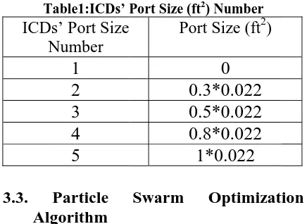
In equation (16), Atotal is cross section of maximum ICDs’ ports size available in the market (manufacturer can make it- here is 0.022 ft2) and Achoke is the required cross section of ICDs which should be acquired through reservoir simulator and optimization algorithm.
Suppose T is production duration and a horizontal well is equipped with N numbers of ICDs. There are infinite situations and combinations for port sizes of ICDs. Hence; in this study we reduce the numbers of combinations through Experimental Design methods to train Neural Network. By then; the optimum port sizes are obtained via Particle Swarm Optimization (PSO).
3. Solution procedure
In this section we elaborate the role of Neural Network as a replace for reservoir simulator, Particle Swarm Optimization Algorithm, and Central Composite Design of kind of Response Surface method to select the samples. Figure 1 shows the solution procedure.
3.1.Structure of artificial neural network
Neural Network simulates human’s brain in the form of an Artificial System. It consists of many processors [Artificial Neurons) designed regularly (there is a complete graph between each two layers] Harrison. S.J and Marshall. R.F (1991). Neural Network consists of variables such as numbers of layers in one network, activation function for each layer, numbers of neurons in each layer, and connection between neurons. The most important element of neural network is Processing Element. Neurons are organized in the form of layers. ANN consists of three layers as input layer, middle (hidden) layer, and output layer [11].
3.1.1. Selection of training samples
Training samples set includes input data and corresponding output. The selection of appropriate set is important and should be included by many input data. In fact; the quality of output depends on selected training samples in the stage of training.
3.1.2. Validation of estimation function (Meta model) designed by ANN
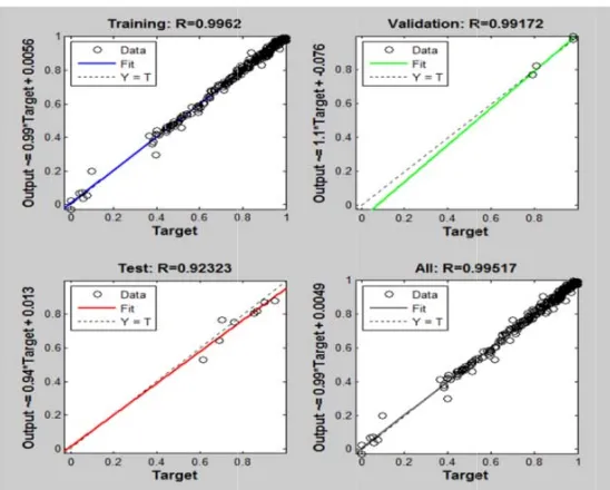
Factors in estimation function designed by ANN are analyzed through regression curves passed over training data, validation data and test data. The numbers of training data, test data and validation data are 80%, 15% and 5% of total data respectively. If Coefficient Of Correlation in regression curve (R2) is near to one it indicates that estimation function has high accuracy. Another method to investigate accuracy of estimation function is Mean Square Error (MSE)with equation 17 Graudenz. S and Bornholdt. D (1992).
2
1
n
i i
i
O T
M S E
n
(17)In this equation (17) Oiis desired (target) output and Ti is ANN outputs for training data, i and n are the numbers of training samples set. Here; the best result is for that ANN with the least MSE Moselhi.T, Fazio.O and Hegazy.P (1994).
3.2. How to select training samples for ANN through Experimental Design method
Experimental Design is a set of tests to realize effective factors on a process and their effectiveness. The applications of this method can be found in identification of effective factors on a process, identification of optimum conditions, process correction in terms of results obtained from feasible conditions, identification of resistant conditions and reduction of variations in process response [5].
To fit quadratic model in RSM there are three applied methods as Central Composite Design (CCD), Box-Behnken Design (BBD) and Doehlert Design. Among these; CCD is the best. By using CCD; better training samples for ANN can be selected. Moreover we could select to training samples by simulator for ANN.
Optimiz the mar on tha mention the num shown continuo discrete to ob accordin number mention training Ta ICDs N
3.3. P Alg Partic was ad This a method (gbest) looking in autho on expe other optimiz their k within PSO a position dispatch position The pa with equ
Vt+1= W
c2. rand
present
In equa paramet
ation of ICDs' P
rket and all at. There ned range. mbers of ca
in Table 1 ous range e range but
tain train ng to the m rs of IC ned range to g samples fo
able1:ICDs’ P s’ Port Size Number 1 2 3 4 5 Particle gorithm cle Swarm dopted from lgorithm i
for solvi problem. for their o orized spac eriences of p
particles ation. Thes knowledge
considered are recogni n and velo hes any p ns [12]. article ident
uations 18 a
Wt. Vt + c1. r
d () (gbest-p
1 t
t presen
ation 18;c ters.rand()
Port Sizes in…
l studies sh are infin CCD helps ases to arbi 1. In fact; of ICDs’ covering c ning samp mathematica CDs; CCD
o 5N differen or ANN.
Port Size (ft2) Port 0.3 0.5 0.8 1 Swarm Optimizati m group fly
is a group ing global
PSO inclu optimum po ce. This pro
particles the to ach se particles over auth d time. The ized in te ocity. Searc
article tow
tifies their and 19.
rand () (pbe presentt)
1
t t
nt V
1
c and c2 is a functio
..
hould be ba nite cases
s us to redu itrarily five
we transfo port size continuous o ples. Hen al model for D transfor nt port sizes
) Number t Size (ft2)
0 3*0.022 5*0.022 8*0.022 *0.022 Optimizat ion Algorit ying of bir p intelligen
optimizat udes partic ositions (pbe ocess is ba emselves or hieve glo are correct horized sp e particles erms of th
ching proc ward optim
next posit
est-presentt)
( ( are learn on for rand
ased in uce e as orm to one nce; r N rms s as ion thm rds. nce tion cles est) ased r of obal ting ace in heir cess mum tion
t) +
18) 19) ning dom gen pr vel con wit equ in
4.
pro in spe fol 4.1 sym wit cha km do aqu preneration o
t
resent andV locity of p ntrol param th respect t uilibrium be the algorith
Figur
Impleme
procedur
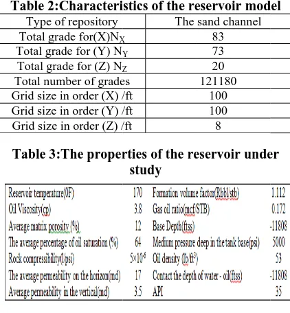
In this sec ocedure onan oil ecifications llowing sect
1. Reservoi
In this stu mmetric a th high annel. The m2 and thick es not have uifer. The esented in T
of number
t
V indicate c particles re meter to ad
to current v etween loca hm [6].
re 1: Solution
entation
re- case st
ction we appa smart hor reservoir are m tion.
r character
udy we hav anticline sa permeabili reservoir d kness of 50 e gas cap a reservoir Table 2 and
r within current posi spectively. djust next velocity and al and globa
n Procedure
of so
tudy
ply aforeme rizontal wel r. The r
entioned
ristics
ve a hetero andstone r ity and dimensions 0 m. The r and it has
characteris d 3. Figure
101
[0, 1]. ition and
t
W is a velocity d creates al search
olution
entioned ll drilled reservoir in the ogeneous reservoir porosity are 44 reservoir a strong stics are102 three-di well equ Table 2 Type Total g Total g Total g Total n Grid siz Grid siz Grid siz Table The this re permeab in the reservoi respecti be obser Figu Fig X imensional uipped with 2:Characteri
e of repository grade for(X)NX grade for (Y ) NY
grade for (Z ) NZ number of grade ze in order (X ) / ze in order (Y ) / ze in order (Z ) /
3:The proper
most imp eservoir a bility. The p
three direc ir in Figure ively. Also,
rved in Figu
ure 2: Three-rese
gures (3-a): C of the perme
the
Journal of Ch
view of sm h ICDs.
istics of the re
The X Y Z es /ft /ft /ft
rties of the re study
portant cha are its p
permeabilit ctions x, y
es (3-a), (3 porosity d ure 4. dimensional rvoir model Cross-section o eability distri e reservoir
hemical and Pe
mart horizon eservoir mod sand channel 83 73 20 121180 100 100 8 eservoir unde aracteristics porosity a ty is illustra
and z in 3-b) and (3 distribution c
views of the
on the axis ibution in etroleum Engine ntal del er of and ated the 3-c) can hor wit firs in hor val is ma acc tot eering, Univers Figures (3 Y of the p
Figures (3 Z of the pe
Figure 4: distr
The hori rizontal sec th 400m d st ICD is lo
middle par rizontal sec lves.
In this stud set to athematical
ceptable wa tal summati
ity of Tehran, V
-b): Cross-se permeability the reserv 3-c): Cross-se ermeability d reservoi Cross-section ribution in th
izontal w ction equipp distance from
ocated in he rt and the t ction. ICDs
dy, the prod 10 years model ater cut is ion of oil pr
Vol. 46, No.2, D
ection on the a y distribution
voir
ection on the a istribution in ir
n of the poros e reservoir
well has ped with thr
m each oth eel part, the third in toe
are fixed p
duction time s. To im the m equal to 60 roduced fro Dec.2012 axis in axis n the sity 1400m ree ICDs her. The e second e part of port size
Optimiz utmost constrai surface water authoriz done by 4.2.Imp ma As p of ICDs sizes to horizon resulting sizes (N situation we pull In this employe named kind o propaga with P General (GRNN particul back pr MLP. Figure 5 Two used to They Regress and wat
ation of ICDs' P
equal to ints are b
production production zed daily o y experts.
plementati athematical
previously m s there are 5 o be investi ntal well is e g to 125 s Note: By ns we cann
the comple s paper; tw
ed to solve as Multilay f feed for ation algori Powell/Beale
lized Regr N) includes
ar linear la ropagation
5: MLP with B with a
o independen o investigat
are Mean sion on resp ter producti
Port Sizes in…
3000 bb based on l n equipmen n and a
oil product
ion of A l model
mentioned; f 5N situations igated. In t equipped w situations f
accepting ot update p etion out of wo neural e the mathe
yer Percept rward train thm (Conju e Restarts ression Neu a radial ba ayer. Figur
algorithm
Back Propag a hidden laye
nt validatio te validity n Square ponses of c on.
..
bl/day. Th limitations nts to han analysis o tion which
ANN on
for N numb s for fixed p this study; with three IC for fixed p one of th port size unl the hole).
networks matical mo tron (MLP) ned by ba ugate Gradi
(CGB)) a ural Netw asis layer a re 5 illustra for error in
gation Algorit r
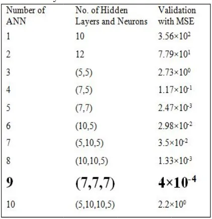
on methods of our wo Method a cumulative hese of ndle over h is the bers port the CDs port hese less are odel ) of ack ient and work and ates n a thm are ork. and oil fro net are net fun Gr Gr (SC In tra wh and eff lay net eva sho hid T du wa hid wit GR MS Ta of
To find an om MLP tworks with e investig tworks in nction (RBF radient (CG radient (CG
CG) and CG all invest ansform fun hich is used
d training a In paralle fect of cha yers and neu twork is aluation th ows how dden layers
Table 4: Effe layer
As Table e to less M ater produc dden layers
th seven ne RNN in co SE (10-6) an able 5 and F
GRNN. n appropria and GRNN h different gated. Inv this study F), Fletcher GF), Polak- GP), Scaled C
GB with dif tigated neu nction is T d for selecti algorithms. el with ab
anges in n urons on M
evaluated. e best one to find th and neuron
ect of various rs and neuro
4 and Figu MSE for c ction the and neuro eurons for e mparison w nd high accu Figures 8 an
ate neural N; various training alg vestigated y are Radi
r-Powell Co Ribiére Co Conjugate G fferent hidde ural netwo Tangent Hy ion of netw
bove inves number of MSE for eac
Based o e is CGB.
e best num ns for CGB.
numbers of ns on CGB
ures 6 and cumulative
best num ons are thre each. It is no
with MLP uracy in reg nd 9 show th
104 Journal of Ch
Figure 6: R production
Figure 7: Be
Figure 8: R and water pr
hemical and Pe
Regression on n for validatio
est fitness (MS
Regression on roduction for
etroleum Engine
n responses of on of meta mo
SE) versus ge
n training res r validation o
GRNN
ANN
eering, Univers
f cumulative odel obtained
eneration
sponses of cum of meta mode
ity of Tehran, V
oil and water d byANNMLP
mulative oil el obtained by
Vol. 46, No.2, D
r
P
y
Optimization of ICDs' P
Figure
Port Sizes in…
Figure 9: water pro
Table 5
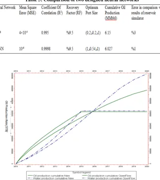
10: Compari theIntellige
..
Regression o oduction for v
5: Compariso
ison of cumul entcontrol (Ne
on test respon validation of
GRNN
ANN
on of two desi
lative oil prod ew) and conv
nses of cumul meta model
igned neural
duction and w ventional (Op
lative oil and obtained by
networks
water levels u pen Flow)
using
106
In thi set and product simulato High good tra to traini
Figure 1
Figu
is work; AN outputs are tion calcu
or.
accuracy in aining and ing data.
Journal of Ch
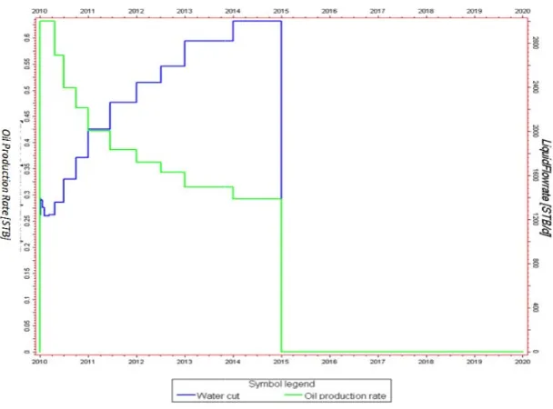
11: The rates
ure 12: The r
NN‘s inputs e cumulative
ulated fro
n above cu convergenc
hemical and Pe
of oil produc
rates of oil pr (co
s are port si e oil and wa om reserv
urves indica ce of test d
etroleum Engine
ction and wat (ANN)
oduction and onventional)
izes ater voir
ates data
4.3 Al
A obt fin 10
eering, Univers
ter cut using
d water cut w
3. Partic gorithm (P
After valid tained by A nd the best p years of pr
ity of Tehran, V
intelligent co
without contro
cle Swarm PSO)
dation of e ANN; PSO
port sizes f roduction.
Vol. 46, No.2, D
ontrol
ol
m Optim
estimation is implem for the ICD
Dec.2012
mization
function mented to
Optimization of ICDs' Port Sizes in….. 107
Indeed; we apply PSO on the Meta model with priority of maximization of cumulative oil production to find the optimum port sizes set. By then; we put Np in interval of
0.09% of Np means [Np-0.0009* Np, Np+0.0009* Np] to find optimum port sizesset based on cumulative water production minimization. Figure 1 shows the solution procedure.
In this study; the optimum port sizes for three ICDs obtained from MLP-CGB are vector of(ICD ICD1, 2,ICD3)(0.2, 0.2,1) . The results for NP and Wp for 10 year production period are 6.15 and 7 MMbbl respectively. Also we put these optimum port sizes in the reservoir simulator. The error between above results and those of reservoir simulator is only three percent. Similarly; the optimum port sizes for three ICDs obtained from GRNN are vector of
(ICD ICD1, 2,ICD3)(1, 0.54,1) . The results for NP and Wp for 10 year production period are 6.027 and 7.05 MMbbl respectively. Also we put these optimum port sizes in the reservoir simulator. The error between above results and those of reservoir simulator is only one percent. Reported errors in Table 5 show that the estimation function could simulate reservoir behavior perfectly. In continuation; we compare above cumulative oil production with one obtained from running reservoir simulator for horizontal well equipped with conventional completion as shown in Figure 10. It shows 55% increase in NP by employing ICDs.
4.4. Comparison of performance of conventional completion with intelligent completion
Figures 11 and 12 show that oil production from intelligent completion
survives within 10 years of study but in the case of conventional completion it dies after 5 years of production. Indeed; lack of control over liquid production causes water production exceeds its limit and consequently shuts the well in.
In this study; recovery factor from conventional and intelligent wells are 6 % and 9.5 % respectively.
5.
Conclusions
In this paper we presented a novel approach for smart well optimization. We elaborated the role of Neural Network as a replace for reservoir simulator, Particle Swarm Optimization Algorithm, and Central Composite Design of kind of Response Surface method to select the samples. The conclusions of this study are as follow:
Considerable increase in oil production from intelligent well with respect to conventional well
Increasing the production period for intelligent well with respect to conventional well
Considerable increase in recovery factor for intelligent well with respect to conventional well.
Acknowledgment
The authors wish to express sincere thanks and appreciation to Research Institute of Petroleum Industry (RIPI) for its help and support particularly Mr, Hendi – Head of Exploration and Production Center-and Mr, Jahanbakhsh- Head of Reservoir Studies Division. Also thank Dr. Ghatee from Amir Kabir University of Technology for its guidance in designing neural network in MATLAB.
References
:
1- Alhuthali, A.H., Gupta, A.D., Yeten, B. and Fontanilla, J.P. (2009). Field applications of
waterflood optimization via optimal rate control with smart well. SPE, Woodlands
108 Journal of Chemical and Petroleum Engineering, University of Tehran, Vol. 46, No.2, Dec.2012
2- Alhuthali, A.H., Gupta, A.D., Yeten, B. and Fontanilla, J.P. (2008). Optimal rate under
geologic uncertainty. SPE, Oklahoma conference.
3- Al-Ghreeb, Z.M. (2009). Monitoring and control of smart wells. Thesis for MSc.
4- Aitokhuehi, I. and Durlofsky, L.J. (2005). "Optimization the performance of smart well in
complex reservoirs using continuously updated geologcal models."Pet. Sci. Eng., pp. 254-264.
5- Beielstein, T.B., Chiarandini, M., Paquete, L. and Preuss, M. (2010). Experimental
Methods for the analysis of optimization algorithms.Springer, Berlin.
6- Eberhart, J. and Kennedy, R. (1995). Particle Swarm Optimization. IEEE, Conference on
Neural Networks.
7- Gao, c., Ranjeswaran, T., Curtin, U. and Nakagawa, E. (2007). A literature review on
smart-well technology. SPE, Oklahoma, March-April.
8- Graudenz, S. and Bornholdt, D. (1992). General asymmetric neural networks and structure
design by genetic algorithms. NeuralNetw, Vol.5. pp. 327-334.
10- Harrison, S.J. and Marshall, R.F. (1991). Optimozation and training of feedforward neural
network by Gas. IEEE Conference on Artificial Neural Network. 39-43.
11- Kamali, M.R., Madadi F, A. and Fakhari, A. (2011). Application of intelligent methods in
Petroleum Engineering and Geosciences. Research Institute of Petroleum Industry (RIPI).
12- Kennedy,C. (2002). The particle swarm Explosion, stability and convergence in a
multideimentional complex space. IEEE, Vol. on Evolutionary Computation, 2002.
13- Moreno, J.C. (2006). Optimization workflow for designing complex wells. SPE, Vienna
Conference.
14- Meun, P., Tondel, P., Godhavn, J.M. and Aamo, O.M. (2008). Optimization of smart well
production through nonlinear model predictive control. SPE, Amsterdam conference.
15- Moselhi, T., Fazio, O. and Hegazy, P. (1994). "Developing practical neural network
applications using back-propagation." Microcomput.Civ., Vol. 9. pp. 145-159.
16- Naus, M.M.J.J., Dolle, N. and Jansen, J. (2005). "Optimization of commingled production
using infinitely variable Inflow Control Valves." SPE, Houston conference.
17- Oberwinker, C., Stundener, M. and Team, D. (2004). From real time data to production
optimization. SPE conference, March.
18- Shuai, Y., White, C.D., Zhang, H. and Sun, T.(2011). using multiscale regularization to
Optimization of ICDs' Port Sizes in….. 109
19- Sobieski, G. and Venter, J. (2002). Particle Swarm Optimization. Structural Dynamics,
and Materials Conference, Denver.
20- Taware, S., Sharme, M., Alhuthali, A.H. and Gupta, A.D. (2010). Optimization water
flood management under geological uncertainty using accelerated production strategy.
SPE, Florence conference.
21- Van Essen, G.M. (2009). Optimization of smart wells in the St.Joseph Field, SPE, Jakarta
conference.
22- Yeten, B., Brouwer, D.R., Durlofsky, L.J. and Aziz, K. (2004). "Decision analysis under
uncertainty for smart well deployment."J. pet. Sci.Eng., pp. 183-199.
23- Yeten, B., Durlofsky, L.J. and Khalid, A. (2002). Optimization of smart well control.