A New Near Optimal High Gain Controller For The Non-Minimum Phase Affine Nonlinear Systems

٭Corresponding Author, Email: [email protected]

A New Near Optimal High Gain Controller For The

Non-Minimum Phase Affine Nonlinear Systems

Hoda N. Foghahaayee

1

, Mohammad B. Menhaj

2

*, and Heidar A. Talebi

2

1- Assistant Professor, Department of Electrical Engineering, Islamic Azad University, Science and Research Branch, Tehran, Iran 2- Professor, Department of Electrical Engineering, Amirkabir University of Technology, Tehran, Iran

ABSTRACT

In this paper, a new analytical method to find a near-optimal high gain controller for the non-minimum

phase affine nonlinear systems is introduced. This controller is derived based on the closed form solution of

the Hamilton-Jacobi-Bellman (HJB) equation associated with the cheap control problem. This methodology

employs an algebraic equation with parametric coefficients for the systems with scalar internal dynamics and

a differential equation for those systems with the internal dynamics of order higher than one. It is shown that

1) if the system starts from different initial conditions located in the close proximity of the origin the

regulation error of the closed-loop system with the proposed controller is less than that of the closed-loop

system with the high gain LQR, which is surely designed for the linearized system around the origin, 2). for

the initial conditions located in a region far from the origin, the proposed controller significantly outperforms

the LQR controller.

KEYWORDS

1. INTRODUCTION

The optimal control of nonlinear systems is one of the difficult and challenging subjects in control theory. The main objective of the optimal control theory is to determine a control input by minimizing or maximizing a proper performance index such that the underlying system keeps satisfying its physical constraints. The two main approaches to solve the optimal control problem are the Variational and the Dynamic Programming approach [1].

The dynamic programming approach is mainly based on the principle of optimality leading to a significant reduction in the time of computations if compared to the global evaluations of all admissible possibilities of a system. This in general is resulted in the solution of the partial differential HJB equation [2]. Due to difficulties in analytic solution of the HJB equation, there is rarely an analytical solution although several numerical computational approaches have been proposed in the literature; i.e., multiple shooting techniques which solve two-point boundary value problems [3, 4], or direct methods [5-7]. More details of the optimal control theory may be found in [8, 9] and [10].

Furthermore, the robust optimal control problems, which have received more attentions in science and engineering since last two decades, were developed in [11-13] for linear systems and in [14] and [15] for nonlinear systems in a linear approximation.

A robust continuous feedback control can be designed using techniques like high-gain feedback, min–max control, or sliding-mode control [16]. High gain feedback control appears to have advantages of good disturbance rejection, good tracking performance, bandwidth increasing and easy realization of decoupling of the input/output variables for the multivariable systems [17].

High gain feedback has gained much interest in singular optimal control problems named cheap control [18-24]. [25] studied the cheap control of non-minimum phase nonlinear systems in the strict-feedback normal form defined in [26]. They used the HJB equation to solve the minimum energy problem for the internal dynamics of the systems with normal strictly feedback form. The internal dynamics in this class of systems is affine with respect to its single input y (the system’s output) as

 

 

0  1 y

 

f



f



where



is the system’s internal states. Due to this property they could easily use HJB equation to find the

minimum energy “y” as the control input to stabilize the origin of internal dynamics.

After that by exploiting the structure of these systems an approximation of the optimal value function, which is indeed O(



)-near-optimal on the basis of the cheap control HJB equation is derived.

In this paper, we propose a new method to approximate a high gain optimal regulator for the special class of non-minimum phase, affine nonlinear systems whose internal dynamics are non-affine with respect to their input “y”. In this technique, we consider a special structure for the cheap control input “u” and then construct an algebraic or differential equation whose solution is used to compute the unknown part of the controller. Note that the near-optimal regulator approximates the optimal regulator in the order of O(ε) [27].

In this study, we focus on the aforementioned class of SISO affine nonlinear systems of relative degree one and will consider whole SISO nonlinear systems in the upcoming paper.

Notice that the method proposed here can be applied to input-output decoupled square MIMO systems. Therefore, to design the optimal high gain state feedback for an MIMO system, we may still apply the proposed method through a suitable input-output pairing method, which is beyond the main scope of the paper.

The rest of the paper is organized as follows. Section 2 presents the preliminary remarks on cheap control along with the HJB equation for linear systems and affine nonlinear systems with affine internal dynamics. An analytical method to compute the solution of the HJB equation and then a near optimal high gain controller for a wide class of affine nonlinear systems is proposed in Section 3. Section 4 presents some illustrative examples and finally, Section 5 concludes the paper.

2. PRELIMINARIES

Consider the following SISO affine nonlinear system with a relative degree of r (r <n) at the origin.

   

 

u y h

 



x f x g x

x

(1)

where _n

x is the state vector and y u,  are the input and output signals respectively.

   

 

1 2

2 3

1

, ,

,

r r

r

z z

z z

z z

z b a u



 



 



z z

q z









(2)

where





1

1 2

T

T r

r

z z z y y y

 _{  }

z and

 



  x such that d

   

_0.

d





x g x x

Here



q z

 

,



is called internal dynamics. The inputs of the internal dynamics are the system’s output and its derivatives. The unforced internal dynamics is zero dynamics which is used to define the minimum phase property as below.

Definition 1 [21]: Nonlinear System (1) with normal form (2) is called minimum phase if the origin of the zero dynamics



q

 

0,



is (globally) asymptotically stable and it is called weakly minimum phase if the origin of the zero dynamics is stable.

Based on this definition a system is said to be non-minimum phase if the origin of its zero dynamics is not stable.

The goal here is to regulate the output of a non-minimum phase system to zero while it should have at least a certain amount of energy to stabilize its internal dynamics. Cheap control methodology can be applied to attain a proper solution for this regulation problem due to the fact that there is no constraint imposed on the input signal. It is well known that any optimal control problem can be reduced to the Riccati (for linear systems) and HJB differential equation (for nonlinear systems) [2].

In this section, we first briefly review the cheap control problem, which can be viewed as a special kind of optimal control problems, for affine nonlinear systems with affine internal dynamics. After that in the next section, we propose a new method to design a near optimal regulator for the affine nonlinear systems with non-affine internal dynamics.:

A. Nonlinear Systems With Affine Internal

Dynamics

Consider the affine nonlinear system (1) with normal form (2) of relative degree 1 and the following cost functional.

 

 



2 2 2



0

1 2

J_ y t  u t dt





_



(3)

The cheap control input to stabilize the nonlinear system (2) and minimize the cost functional (3) is





*

2

1

, V

u a y

y



  





(4)

which is obtained by solving the following HJB equation [12].













2

2 2

2

1

, ,

2 1

, 0

2

V V

y b y y

y

V

a y

y



 _ _

 

 

 _{ } 

  

 





q

(5)

In order to solve this equation, we can use an approximate solution of V on the optimal trajectory,

* *

,

y



, given bellow



* *



 

*



* *

  

2

0 1

; , ,

V  y  V  V y  O  (6)

By substituting (6) into (5) it becomes obvious that we need one extra equation to find the Vi (i=0,1 …) terms. To do so, for the systems with affine internal dynamics,

 

* 0

V  is determined by employing the minimum energy

problem of internal dynamics. For the sake of simplicity, from now on the symbol“*” is omitted.

Now, consider the affine nonlinear system (2) with the affine internal dynamics

 

 

0  1 y

  f  f 

₍₇₎

The HJB equation (5) for this system becomes







 

 











0 1

2

2 2

2

,

1 1

, 0

2 2

V V

b y y

y

V

y a y

y



 _ _

 

 

  _{ } 



 

  





f f

(8)

It is well-known that this problem has a solution for each



0,if there exists a C1 positive semi-definite function

V y



, ,







such that the state feedback control (4) globally asymptotically stabilizes the origin of system (2) [32]. The solution of this problem when



0 hinges upon the solution to the following minimum energy problem, where the system output is treated as the control variable: Find “y” to asymptotically stabilize the origin of the internal dynamics (7) and to minimize the cost functional

 

2

0

1

2

J

_

y

t dt





_

(9)

Now, if there exists a C1 positive definite function

 

0

     

0 0 0

0 1 1

1

0 2

T T

V V V

  

 

 f   f  f  

(10)

such that

    0

1 T

T V

y    



 



f

₍₁₁₎

globally asymptotically stabilizes the origin of the internal dynamics (7) then (11) is the optimal control and V₀

 



is the optimal value function. Now the control input signal

 





1

u y





 _

_

(12)

is the approximate cheap control input, which stabilizes the origin of system (2).

The optimal output signal for the systems with scalar internal dynamics (



) becomes

 

_{ }

0

 

1

2

f

y

f



 









(13)

and therefore the near optimal high gain control input is

obtained as

 

 

0 1 1 2f u y f        _  _   .

3. NEAR OPTIMAL HIGH GAIN CONTROLLER FOR THE

SPECIAL CLASS OF NONLINEAR SYSTEMS

Now, in this section we propose an analytical method to solve cheap control HJB equation (5) for a class of affine nonlinear systems with non-affine internal dynamics. According to this method we are looking for a closed form optimal output signal as a function of internal states. We should note that for this special class of systems, it is almost impossible to obtain an analytical solution for the minimum energy problem.

Now consider the affine nonlinear system (2) with relative degree one and the internal dynamics of form

 

 

 





1 1 2 2 2 2

1 1 ,

n n n n q q q q y                 _   _     

(14)

We are interested to find an optimal high gain control of the form

 



 



1

,

c

u



y

y















(15)

where  

 

is a smooth function of the internal states. Note that (15) is in fact an approximation of (4) which should satisfy (5).

In order to find the near optimal control input (15) the following assumption is crucial.

Assumption 1- There is a finite positive number m such that the following expression gives a reasonable approximation of

q

_n1



y

,





.

 

 

 

 

1

,

0 1

,

1

m

n m

q

_

y



f





f



y

 

f



y

m



where

 

 

 

 

1 0 0 1

,

1

,

0

!

0,

k n k k y n

q

y

f

k

k

y

f

q

  





 













Now consider the affine nonlinear system with the normal form

   

 

 

 

 

 

 

1 1 2 2 2 2

1 0 1

, , ,

, 1

n n

m

n m

y b y a y u

q q

q

f f y f y m

                   _                

(16)

where

 

 

0 0

, , p, 0 , 0 .

y u  y y  

The main goal is to solve the cheap control problem (i.e., the HJB Eq. (5)) for  

 

through the optimal high gain control input signal (15). Now, use the approximate solution of V given in (6) and then write the HJB Eq. (5) as    

_{ }

_{ }    

_{ }

_{ }    

 

     





 

_{ }

_{ }      

0 1 2

1

1 1

0 1 2

2 2 2 0 1 1 0 1 1 2 1 2 2 1 2 2 , 2 , 2 , 2 , 2 , , , 0 n n n n m m n

V V y

O q

V V y

O q

V V y

f f y f y

O V y

O b y

y

V y

y a y O

y                           _{ }          _  _        _     _                          _          _           _         

(17)

which can be easily rewritten as









2





 

3

0 , 1 , 2 , 0

p y p y  p y O  

₍₁₈₎

Now by setting ε to zero, (17) reduces to





   

 

 

     



 











0 0

0 1 2

1 2 0 0 1 1 2 1 2 2

, 2 2

2 , , 0 n n m m n V V

p y q q

V

f f y f y

V y

y a y

y                         _               

(19)

By substituting (6) into (4) we have

 

1

 

1

, V

u a y O

y       _  _    

(20)

Use (20) and (15) and after some algebraic manipulations to write











 



1 , , c y V y y a y

   _{ }    

(21)

Substitute (21) into (19) and obtain:

   

 

_{ }

     



 



 



 



0 0 1 2 1 2 0 0 1 1 2 2 2 2 2 2 , 0 n n m m n c V V q q V

f f y f y

y y y

                                 

(22)

Knowing that the closed-loop system through the cheap control input (15) is indeed a singular perturbation system represented as







 





 



 

 

 

 

 

 

1 1 2 2 2 2

1 0 1

, , , , , 1 c n n m n m

y b y a y y y

q q

q

f f y f y m

                        _   _{    }           

according to the singular perturbation’s theorem [33], the fast dynamics, y, through a fast transient response is laid on the following slow manifold and stayed there forever.

 

y





(23)

Knowing that the HJB equation is only for optimal trajectories, the solution (23) should satisfy (22) and its all derivatives. By substituting (23) into both (22) and the first derivative of (22), the equations (24) and (25) are derived respectively.

 

   

 

 

 

_

_{ }

_{   }

_{   }

_

2 0 0

1 2 1 2 0 0 1 1 2 2 0 n n m m n V V q q V

f f f

                                       

(24)

   



 

1

 



 

0

1 1

2 m 2 0

m n

V

f mf  

             

(25)

The following equation easily follows from (25).

 

 

 

 

 





0 1 1 1 m n m V f mf             

  

(26)

Now, substitute (26) into (24) to obtain

   

 

_{ }

   



   

   



 

 

 





 

0 0 1 2 1 2 0 1 1 1 2 2 2 0 n n m m m m V V q q

f f f

f mf                                             

(27)

Dividing equation (27) by equation (43.14) and using the following fact

 

 

 

 

0 0

i i

V V 

             

we obtain the following differential equation.

   

 

_{ }

 

   

   





   



 

 



 

1 2 1 2 0 1 1 1 1 1 2 n n m m m n m q q

f f f

f mf       _                   _    _{ }                 _    

(28)

For the system (16) with the scalar internal dynamics, (n=2), the differential equation (28) is reduced to an algebraic equation of the form

 

   

   





   



 

 



0 1 1 1 1 0 2 m m m m

f f f

f mf

      

      

   

   

which in turn yields

 

   

   



    

3

0 1 3

2

2 m 0

m

f f f

m f



  

  

  

 

   

(29)

Now, for the system (16) with n=2 and m=1 (i.e., the affine nonlinear system in strictly feedback form) the solution of (29) can be easily obtained as

 

_{ }

0

 

1 2f f     

The following lemma shows that for nonlinear system (16) the first term of the approximate cost value function V given in (6) is indeed the amount of energy of the optimal output signal.

Lemma 1: Consider affine nonlinear system (1) with

 

0 0, h

 

0 0

f and well-defined normal form (16). The value function

 

0

V  is

 





2

0

1

2



t

dt







where



 

_t

is the response of the differential equation

 





,







q

 

with initial value



.and

 

 

is a function satisfies (28).

Proof: Using the fact that

V





; ,

y





is the value function of cost functional (3), it could be written as





 

 

 

 

 





2

0 1

2 2 2

0

; , ,

1 2

V y V V y O

y t u t dt











  



_









(30)

where

y

,



are the optimal trajectories. By substituting optimal control input (20) in (30) and using (21), we have





 





 

 





_



_





 



 

2

0 1

2

2 2

0

; , ,

, 1

,

2 ,

c

V y V V y O

y

y t a y y O dt

a y

  

 _{ }



  

 _{ } 

 

 _  _   _{ }

 

 



  



 



Here by replacing the optimal trajectory y from (23), the value function V when 1becomes





 





 

 

 





 

 

2

0 1

2 2 2

0 0

; , ,

1 1

2 2

V y V V y O

O dt dt O

  

   

 

  



_

 

_



  

 

Therefore, it can be easily concluded that

 

2

 

0

0

1 2

V



dt











Notice that



in above is the initial value of the internal states.

Theorem 1: Consider affine nonlinear system (1) with normal form (16). The origin of the internal dynamics of system (2) becomes asymptotically stable through the output signal

y





 



if

 

 

satisfies dynamical equation (28) and also 

 

₀ ₀.

Proof: In order to prove the asymptotic stability of the internal dynamics we choose cost value function

 

0 V



as the Lyapunov function. From the Lyapunov’s second method for stability [26], the origin of the internal dynamics is (locally) asymptotically stable if

 

0 0

V  

for every nonzero



 

t

(located in a neighborhood of the origin) and

 

0 0

V   at the origin. Now,

 

0 V  is computed as

 

 

   

 

_

_{ }

_

1 0 0

1

2

0 0

1

1 1

, n

i

i i

n

i n

i i n

V d

V

dt

V V

q q











  



 

 



 

 

 















 

Knowing that

 

 

satisfies (28), thus it surely satisfies (24), (25) and finally it should satisfy equation (22) through

y





 



. By substituting

y





 



into (22) it becomes

   

 

_

_{ }

_

_{ }

0 1 1

0 2

1 1

2

2 _n , 0

n

V q

V q















 



  









 



and then

 

   

 



 



 

2

0 0

0 1

1 1

2

,

1 2

n

i n

i i n

V V

V q q 

 







 

 

 

 

 



 

   



which is negative for all nonzero



(located in a neighborhood of the origin) and this in turn leads to the (locally) asymptotic stability of the origin of the internal dynamics and simply completes the proof.

Now to find the proportional approximate cheap control input (24), we in fact need to compute the functional coefficient



_c



y

,





. To do so, we assume that for the square of this functional the following power series expansion is given





 

 

 

 

2

0 1

3 3

,

, max 3,

c

l l

y n n y

n y l m



 

 

  









(31)

   

 

_{ }

 

 

 

 

 

 





 

 

 



 

 



0 0 1 2 1 2 0 0 1 1

0 1 2 2

3 3 2 2 2 2 0 n n b m m n t t V V q q V

f f y f y

n n y

y y n y y                  _{ }             _ _                       

(32)

Now, (32) can be simply rewritten as

 

 

 

0 1 0

m m

s



s



y s



y 

(33)

where

s

_is are computed from the following equations.

 

 

   

   

 

   

   

   

 

   

 

   

   





 

   

 

   

   





 

   

 

 

 

   





 

 

 

 

 

   

2

0 0 0

2

1 1 0 1

2 2

2

0 1 2

3 3

2

1 2 3

2

2 1

1 1 3

2 1 2 2 2 k k

k k k

m m m

m m

s b f n

s f n n

s f

n n n

s f

n n n

s f

n n n

s f n

s f                                                                                       

(34)

According to the fact that only the optimal trajectory_y

 

 satisfies the HJB equation, by replacing

y

with

 

 

in (33) and its first m-1 derivatives, the coefficients

s

_is are easily computed from the following equation.

 



1

 

1

  

,

!

1, ,

k

m k m

m m m k

s s k k m         

(35)

where

 

   

m m

s    f  .

Now from (34) the coefficients of



_c2



y

,





are determined as                   1 1 1 1 1 !

1 ! 1 !

1, , k j k m j mk j j m k j f n m f

j m j

k m           _               _{ } _{ }           

 

₍₃₆₎

Remark 1: For the system (1) with relative degree r>1, we first reduce the system’s relative degree to one and then employ the proposed algorithm to design the near-optimal controller.

To do so, the following simple output redefinition is used.

 2  1

1 1

r r

new r

y



c y

 

c

_

y





y



(37)

where

c

₁

,

,

c

_r1 are the coefficients of a Hurwitz polynomial such as

 

1 2

1 1

r r

r

p s s c s_   c . The normal form of system (1) through this output redefinition becomes













1 2

2 3

1 1 1 1 1

,

,

,

new n new new n new new

n new s

r r r new

y

b

y

a

y

u

y

z

z

z

z

z

_

c z

c

_

z

_

y











 

 









q

z ,



(38)

where



1 1



,

T T

T T

new s  s z zr

  z z

and









 





 





 

1 1 1 1 1 1 1 1 1 1 1 1

1 2 2 1

1 1 1 1 1

,

,

,

,

r r r new

r r r new

r r r new

n new new r r

r r r new

z c z c z y

n new new _{z c z c z y}

n new new _{z c z c z y}

b

y

c z

c

z

c

c z

c

z

y

b

a

y

a

y

q

                      



 



 





















z

z

q

z

Here the internal dynamics is





1 2

2 3

1 1 1 1 1

,

n new s

r r r new

y

z

z

z

z

z

_

c z

c

_

z

_

y







 

 





q

z ,



the near optimal high gain controller is only designed for



,



n ynew s



 q z , .

Below we present some illustrative examples to clarify better the merit of the proposed controller..

4. ILLUSTRATIVE EXAMPLES

Example 1- Consider the following affine nonlinear system:





 

2 2

2

10 cos

y y u

y y



 





   



 _{   }



where y is its output and



is its internal state. The zero dynamics of the system is

 



. Obviously, the system is non-minimum phase because the origin of its zero dynamics is unstable. The solution of equation (29) for this system is simply given as

 

2

10   



 

 and the

coefficient



_c

 

y

,



equals 1. Therefore from (15), the near optimal high gain controller (NOHGC) becomes

1 2

, 0

10

u y  

 

 



 _  _ 



 

The closed-loop system via this controller can be described as





 

2 2

2

2 10

10 cos

y y y

y y



  



   

 _{  } _ 

  _ 

 



    



The fast dynamics of this singular perturbation system is     y/



y O

 



where 2

10

y y 



 

 and

t

 

 . Obviously, the origin of the fast dynamics is asymptotically stable leading to the following equation.

 

2

 

_{ }

 

,

 

10

t

y t O t T

t



 





  



Note that

T

 



is a very small positive number of order



. According to the stability theorem of the singular perturbation systems [33], the origin of the closed-loop system is asymptotically stable provided that the origin of its slow and fast dynamics are both asymptotically stable. The slow dynamics of this system is

 

2 2 cos

10



  



 

   _{ }



 

(39)

It can be easily shown that the origin,





0

, is asymptotically stable provided that the initial value of the internal state satisfies

0 5.5

   ; this in turn leads to the

local asymptotic stability of the origin



y0,0



of the

closed-loop system. Furthermore, for other initial conditions there exist two stable equilibrium points

1,2

(  7.7, 13.8) , and two unstable ones

3,4

(  5.5, 11) ; this will guarantee the bounded-ness of the solution of the closed-loop system for a wide range of initial conditions, see Figure 1.

For the sake of comparison, we design a high gain LQR controller (HG-LQR) for the system. To do so, the linearized system around the origin is obtained as

10

y

u

y









 





For the cost functional (3) with



1

, the optimal state feedback controller will tend to 1

5

LQR

u y





 

  _  _  . The slow dynamics of the closed-loop system is

 

2

2

cos

5 5







  







 _{ }

 

(40)

The origin of the closed-loop system through the HG-LQR controller is asymptotically stable for the initial conditions

0 4.9

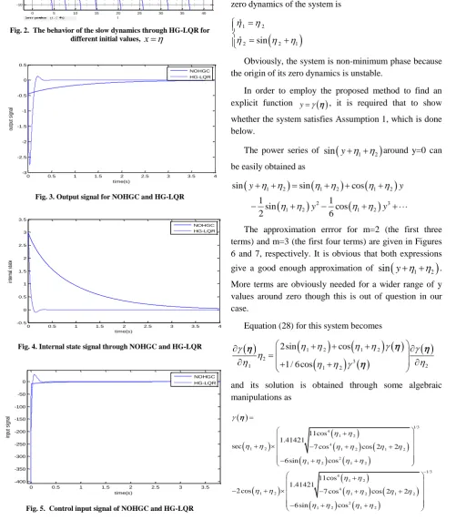
   while the system’s solution becomes unbounded for the other initial conditions (there is only one equilibrium point near the point ( 5,y1) which is unstable). The simulation results are illustrated in Figures 3, 4 and 5 for the initial conditionsy0,



3,

and 3

10



_  _{. It seems that the regulation error norm of} NOHGC is significantly less than that of HG-LQR.

0 1 2 3 4 5 6 7 8 9 10

-50 -40 -30 -20 -10 0 10

time(s)

x

x ' = - x - cos(x) (2 x/(x + 10))2

0 5 10 15 20 25 30 35 40 -10

-8 -6 -4 -2 0 2 4 6 8 10

t

x

x ' = x + (10 + x) ( - 2 x/(10)) - cos(x) ( - 2 x/(10))2

Fig. 2. The behavior of the slow dynamics through HG-LQR for different initial values, x



0 0.5 1 1.5 2 2.5 3 3.5 4

-3 -2.5 -2 -1.5 -1 -0.5 0 0.5

time(s)

ou

tp

ut

s

ig

na

l

NOHGC HG-LQR

Fig. 3.Output signal for NOHGC and HG-LQR

0 0.5 1 1.5 2 2.5 3 3.5 4

-0.5 0 0.5 1 1.5 2 2.5 3 3.5

time(s)

in

te

rn

al

s

ta

te

NOHGC HG-LQR

Fig. 4.Internal state signal through NOHGC and HG-LQR

0 0.5 1 1.5 2 2.5 3 3.5

-400 -350 -300 -250 -200 -150 -100 -50 0

time(s)

in

pu

t s

ig

na

l

NOHGC HG-LQR

Fig. 5. Control input signal of NOHGC and HG-LQR

Example 2- Consider the following affine nonlinear system.









2 2 2

1 2

1 2

2 1 2

4 1

sin

y y y y u

y















     

 _  

  



where y is its output and

1, 2

 

are its internal states. The zero dynamics of the system is





1 2

2 sin 2 1











 

 _{ }



Obviously, the system is non-minimum phase because the origin of its zero dynamics is unstable.

In order to employ the proposed method to find an explicit function _y

 

_ , it is required that to show whether the system satisfies Assumption 1, which is done below.

The power series of

_sin



_y

 

 

_{1 2}



around y=0 can be easily obtained as





















1 2 1 2 1 2

2 3

1 2 1 2

sin sin cos

1 1

sin cos

2 6

y y

y y

 

 

 

 

 

     

    

The approximation errror for m=2 (the first three terms) and m=3 (the first four terms) are given in Figures 6 and 7, respectively. It is obvious that both expressions give a good enough approximation of

sin



y

 

 

_{1 2}



. More terms are obviously needed for a wider range of y values around zero though this is out of question in our case.

Equation (28) for this system becomes

 









 





 

 

1 2 1 2

2 ₃

1 _{1 2} 2

2sin cos

1/ 6 cos

    

 



 _{  } 

    

 _{ }



 

 _{ } 

 



 



and its solution is obtained through some algebraic manipulations as

 











 





















 











1/3 4

1 2 4

1 2 1 2 1 2

2

1 2 1 2

1/3 4

1 2 4

1 2 1 2 1 2

2

1 2 1 2

11cos 1.41421

sec 7 cos cos 2 2

6 sin cos 11cos 1.41421

2 cos 7 cos cos 2 2

6 sin cos



 

     

   

 

     

   

 

 _ 

 

 

 _    _

 

   

 

 _ 

 

 

  _    _

 

   

 

For this system, the coefficient



_c

 

y

,



equals 1. Now from (15), the NOHGC becomes _u 1



_{y }

 







   . Obviously, the slow dynamics of the closed-loop system becomes

 





1 2

2 sin 1 2

 



 



 

 _{  }





(41)

The phase plane diagram of the slow dynamics (41) is shown in Figure 8.

Now the linearized system around the origin is

2

1 2

2 1 2

y u

y



 



 

 

   

    

For the cost functional (4) with





10

3, the HG-LQR controller becomes



1 2



1000 1.003 2.003 +3.24

LQR

u   y





The slow dynamics of the closed-loop system through the above control input is





1 2

2 sin 1 2.24 2

 

  

 

 _{  }



(42)

Figure 9 shows the region of attraction of the origin,

 

 , due to the LQR controller.

According to the Figures 8 and 9 we cannot say that the region of attraction of the origin through the proposed controller is bigger than that of the HG-LQR controller; however, some simulation results show that the regulation error norm of NOHGC is less than that of HG-LQR.

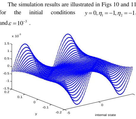
The simulation results are illustrated in Figs 10 and 11 for the initial conditions

1 2

0, 1, 1

y       ,

and 3

10 _  _.

-5

0

5

-0.2 -0.1 0 0.1 0.2 -1.5 -1 -0.5 0 0.5 1 1.5

x 10-3

internal state y

Fig. 6.Approximation error for m=2

-5

0

5

-0.2 -0.1 0 0.1 0.2

-1 -0.5 0 0.5 1

x 10-4

internal state y

Fig. 7.Approximation error for m=3

x1 ' = x2 x2 ' = sin(x1 + x2 + M - 2 M( _{- 1))}

M = sec(x1 + x2) (sqrt(22 cos(x1 + x2)4 _{- 14 cos(x1 + x2)}4 _{cos(2 (x1 + x2))) - 6 sin(x1 + x2) cos(x1 + x2)}2₎(_1/3)

-4 -3 -2 -1 0 1 2 3 4

-4 -3 -2 -1 0 1 2 3 4

x1

x2

Fig. 8.Phase plane diagram of the slow dynamics given in (41) where x_i_i

x1 ' = x2

x2 ' = sin(x1 + x2 + - 66.48/34.86 x1 - 107.57/34.86 x2)

-4 -3 -2 -1 0 1 2 3 4

-4 -3 -2 -1 0 1 2 3 4

x1

x2

Fig. 9.Phase plane diagram of the slow dynamics given in (42) where

i i

x 

0 1 2 3 4 5 6 7

-1 0 1 2 3 4 5

time(s)

ou

tp

ut

s

ig

na

l

NOHGC HG-LQR

0 1 2 3 4 5 6 7 -400

-300 -200 -100 0 100 200

time(s)

co

nt

ro

l i

np

ut

s

ig

na

l

NOHGC HG-LQR

Fig. 11.Control input signal through NOHGC and HG-LQR

5. CONCLUSIONS

In this paper, a new analytical method to design an optimal high gain controller for the affine nonlinear systems was introduced. To find this controller an approximate closed form solution of the HJB equation associated with the cheap control problem was computed. The HJB equation was solved by using of an algebraic equation for the systems with scalar internal dynamics and a differential equation for those with the internal dynamics of higher order than one.

Finally through some examples, it was shown that the regulation error of the closed-loop system via the proposed optimal high gain controller is significantly lower than that of the closed-loop system using the high gain LQR which is surely designed for the linearized system around the origin.

REFERENCES

[1] J. B. Lasserre, C. Prieur, and D. Henrion. “Nonlinear optimal control: numerical approximation via moments and LMI relaxations. in joint,” IEEE Conference on Decision and Control and European Control Conference, 2005. [2] J. Arthur, E. Bryson, and Y.-C. Ho, Applied

Optimal Control: Optimization, Estimation and Control: Hemisphere Publ. Corp., Washington D.C, 1975.

[3] W. Grimm and A. Markl, “Adjoint estimation from a direct multiple shooting method,” Journal of Optimization Theory and Applications, vol. 92, No. 2, pp- 263–283, 1997.

[4] J. Stoer and R. Bulirsch, Introduction to Numerical Analysis, ed. T. Edition, New York: Springer-Verlag, 2002.

[5] O. v. Stryk and R. Bulirsch, “Direct and indirect methods for trajectory optimization,” annals of operations research, vol. 37, No. 1, pp-357–373, 1992.

[6] R. Fletcher, Practical methods of optimization: Unconstrained optimization, John Wiley & Sons, Ltd., Chichester, 1980.

[7] P. E. Gill, W. Murray, and M. H. Wright, Practical optimization. : Academic Press, Inc., London-New York, 1981.

[8] D. E. Kirk, Optimal Control Theory: An Introduction, Prentice-Hall, Englewood Cliffs, NJ: Dover Publications, USA, 1998.

[9] D. S. Naidu, Optimal Control Systems: CRC Press, Idaho State University, USA,, 2003.

[10] S. Subchan and R. Zbikowski, computational Optimal Control: Tools and Practice, United Kingdom: John Wiley & Sons, 2009.

[11] K. Zhou, J. C. Doyle, and K. Glover, Robust and optimal control: Prentice Hall, Englewood Cliffs, NJ, 1996.

[12] A. Ben-Tal and A. Nemirovski, “Robust Convex Optimization,” Mathematics of operations research, vol. 23, No. 4, pp-769-805, 1998.

[13] A. Ben-Tal and A. Nemirovski, “Lectures on Modern Convex Optimization: Analysis, Algorithms, and Engineering Applications,” MPS-SIAM Series on Optimization. MPS-MPS-SIAM, Philadelphia, 2001.

[14] Z. K. Nagy and R. Braatz, “Open-loop and closed-loop robust optimal control of batch processes using distributional and worst-case analysis,” Journal of Process Control, vol. 14, No. 4, pp-411– 422, 2004.

[15] M. Diehl, H. G. Bock, and E. Kostina, “An approximation technique for robust nonlinear optimization,” Mathematical Programming, vol. 107, No. 1-2, pp-213–230, 2006.

[16] S. Seshagiria and H. K. Khalilb, “Robust output feedback regulation of minimum-phase nonlinear systems usingconditional integrators,” Automatica, vol. 41, No. 1, pp-43 – 54, 2005.

[17] H. Nogami and H. Maeda, “Robust Stabilization of Multivariable High Gain Feedback Systems,” Transactions of the Society of Instrument and Control Engineers, vol. E, No. 1, pp- 83-91, 2001. [18] W. Maas and A. v. d. Schaft. “Singular nonlinear

Hinf optimal control by state feedback,” in 33th IEEE conference on decision & control. Lake Buena Vista, USA, 1994.

[19] A. Astolfi. “singular Hinf control,” in 33th IEEE conference on decision and control. Lake Buena Vista, USA, 1994.

[21] A. Isidori, nonlinear control systems. third ed, Berlin: Springer Verlag, 1995.

[22] A. Isidori, “Global almost disturbance decoupling with stability for non minimumphase single-input single-output nonlinear systems,” systems & control letters, vol. 28, No. 2, pp-115-122, 1996. [23] B. Achwartz, A. Isidori, and T. Tarn. “Performance

bounds for disturbance attenuation in nonlinear nonminimum-phase systems,” in European Control Conference Brussels, Belgium, 1997.

[24] M. Seron, et al., Feedback limitations in nonlinear systems: From Bode integrals to cheap control, University of California: Santa Barbara, 1997. [25] M. M. Seron, et al., “Feedback limitations in

nonlinear systems: From bode integrals to cheap control,” IEEE Transactions on Automatic Control, vol. 44, No. 4, pp-829–833, 1999.

[26] M. Krstic', I. Kanellakopoulos, and P. Kokotovic', Nonlinear and adaptive control design: John Wiley & Sons, 1995.

[27] J. W. Helton, et al., “Singularly perturbed control systems using non-commutative computer algebra,” International Journal of Robust and Nonlinear Control, Special Issue: GEORGE ZAMES COMMEMORATIVE ISSUE, vol. 10, No. 11-12, pp- 983–1003, 2000.

[28] H. Kwakernaak and R. Sivan, Linear Optimal Control Systems, New York, Chichester, Brisbane, Toronto: Wiley-Interscience, a division of John Wiley & Sons, Inc, 1972a.

[29] H. Kwakernaak and R. Sivan, “The maximally achievable accuracy of linear optimal regulators and linear optimal filters,” IEEE Transactions on Automatic Control, vol. 17, No. 1, pp-79-86, 1972b.

[30] U. Shaked, Singular and cheap optimal control: the minimum and nonminimum phase cases, National Research Institute for Mathematical Sciences: Pretoria, Republic of South Africa, 1980.

[31] A. Jameson and R. E. O'Malley, “Cheap control of the time-invariant regulator,” applied mathematics & optimization, vol. 1, No. 4, pp-337-354, 1975. [32] R. Sepulchre, et al., Constructive nonlinear control,

Springer, Editor: London, 1997.