www.biogeosciences.net/9/4819/2012/ doi:10.5194/bg-9-4819-2012
© Author(s) 2012. CC Attribution 3.0 License.
Biogeosciences
Changes in column inventories of carbon and oxygen in the
Atlantic Ocean
T. Tanhua1and R. F. Keeling2
1Department of Marine Biogeochemistry, GEOMAR Helmholtz Centre for Ocean Research Kiel, Kiel, Germany 2Geosciences Research Division, Scripps Institution of Oceanography, University of California San Diego, La Jolla, CA, USA
Correspondence to: T. Tanhua ([email protected])
Received: 15 June 2012 – Published in Biogeosciences Discuss.: 3 July 2012
Revised: 25 October 2012 – Accepted: 9 November 2012 – Published: 26 November 2012
Abstract. Increasing concentrations of dissolved inorganic
carbon (DIC) in the interior ocean are expected as a di-rect consequence of increasing concentrations of CO2in the atmosphere. This extra DIC is often referred to as anthro-pogenic carbon (Cant), and its inventory, or increase rate, in the interior ocean has previously been estimated by a multi-tude of observational approaches. Each of these methods is associated with hard to test assumptions since Cantcannot be directly observed. Results from a simpler concept with fewer assumptions applied to the Atlantic Ocean are reported on here using two large data collections of carbon relevant bot-tle data. The change in column inventory on decadal time scales, i.e. the storage rate, of DIC, respiration compensated DIC and oxygen is calculated for the Atlantic Ocean. We re-port storage rates and the confidence intervals of the mean trend at the 95 % level (CI), reflecting the mean trend but not considering potential biasing effects of the spatial and temporal sampling. For the whole Atlantic Ocean the mean trends for DIC and oxygen are non-zero at the 95 % confi-dence level: DIC: 0.86 (CI: 0.72–1.00) and oxygen:−0.24 (CI:−0.41–(−0.07)) mol m−2yr−1. For oxygen, the whole Atlantic trend is dominated by the subpolar North Atlantic, whereas for other regions the O2trends are not significant. The storage rates are similar to changes found by other stud-ies, although with large uncertainty. For the subpolar North Atlantic the storage rates show significant temporal and re-gional variation of all variables. This seems to be due to variations in the prevalence of subsurface water masses with different DIC and oxygen concentrations leading to some-times different signs of storage rates for DIC compared to published Cantestimates. This study suggest that accurate
as-sessment of the uptake of CO2by the oceans will require ac-counting not only for processes that influence Cant but also additional processes that modify CO2storage.
1 Introduction
The ocean has stored a large fraction of the CO2emitted by human activities over the last few hundred years, i.e. the an-thropogenic CO2(Cant). A major scientific challenge today is to assess the oceanic sink and storage of CO2. It is there-fore relevant to monitor the storage rate of dissolved inor-ganic carbon (DIC) in the ocean and to assess its sensitivity to (climate-induced) changes in circulation and biology. Much of prior work has focused on determining the total oceanic uptake of CO2 in the ocean due to increasing atmospheric CO2 concentrations, i.e. changes related to the thermody-namic air–sea disequilibrium driven by atmospheric changes (i.e. Cant). Changes in oceanic CO2content due to changes in the ocean carbon cycle driven by other internal ocean fac-tors that impact air–sea exchange of CO2, such as changes in circulation or productivity/respiration, are most often not considered. Over long time scales and over large areas, the Cantcomponent has so far been dominating over the changes in DIC due to increase in the concentration of Cant, although on smaller spatial and temporal scales the natural variability can dominate.
to as “repeat hydrography”. It has been shown that the stor-age rates calculated from repeat hydrography can be scaled to encompass the full Cantinventory in the North Atlantic by as-suming steady state circulation and transient steady state be-havior of the anthropogenic carbon (e.g. Tanhua et al., 2007; Gammon et al., 1982), and that the Cantconcentration in the surface ocean is, to a first approximation, exponentially in-creasing. In principle, the change in DIC concentration be-tween repeat measurements (i.e.1DIC) at a specific loca-tion and depth in the ocean can be assumed to represent the anthropogenic component, which can be integrated over the water column to assess the storage rate of anthropogenic car-bon. However, a direct comparison of the DIC fields usu-ally show large variability, i.e. a patchy image, of the decadal change in DIC (or any other property) concentrations due to spatial and temporal variability in the ocean such as eddies and variable location of ocean fronts (e.g. Wanninkhof et al., 2010).
A common approach to estimate Cantinvolves combining DIC data with dissolved O2or nutrient data to reduce vari-ability due to internal ocean processes such as changes in remineralization. The variable effect on DIC is assumed to be captured from other tracers assuming fixed elemental ratios (C/N, C/P, C/O, i.e. Redfield ratios). A related approach uses multiple linear regressions (MLRs) where relations between a number of relevant properties, such as nutrients, oxygen and salinity are used to determine the DIC concentration of the sample. The use of MLR has the capacity to compensate for some of the small scale variability in the ocean and the result is usually relatively smooth fields of1DIC. A varia-tion of the MLR method was suggested by Friis et al. (2005) in which the MLR coefficients for both the cruise are sub-tracted from each other and then directly used for the cal-culation of the1DIC. This approach is known as extended MRL (eMLR). Wanninkhof et al. (2010) finds significant bi-ases and various amount of scatter in the 1DIC fields de-pending on the method applied to a section through the At-lantic Ocean, indicating that the correct choice of methodol-ogy is critical. A thorough analysis of potential biases in the MLR method is provided by Levine et al. (2008), where par-ticularly potential biases in the deep water formation regions were pointed out.
Furthermore, estimates of Cant that use O2 as a compo-nent of tracer combination are subject to an easily understood bias. The integration of the tracer combination over the col-umn to yield the change in the inventory of Cantyields a sum of terms, one for inventory of each of the components, in-cluding the O2inventory. Globally, the change in O2 inven-tory, however, is largely controlled by air–sea exchanges of O2(Keeling and Garcia, 2002). Thus a combined tracer that includes O2 will be sensitive not just to processes driving long-term uptake of CO2by the oceans, but also processes driving long-term changes in O2(Keeling, 2005; Yool et al., 2010). Recent studies suggest that the change in global ocean O2inventory is decreasing at the level of∼50 Tmol yr−1due
to warming and increased ocean stratification (Keeling et al., 2010; Helm et al., 2011), which is significant compared to estimated global ocean CO2uptake of ∼200 Tmol yr−1. A tracer combination that uses O2therefore cannot yield a reli-able estimate of ocean CO2uptake unless it is combined with independent estimates of the changes in ocean O2inventory (Keeling et al., 2010). Estimates of Cantthat include potential temperature as a correlating variable will be similarly sensi-tive to changes in ocean heat content (Levitus et al., 2012).
Related problems have been documented locally. For in-stance, time series data from the DYFAMED site in the West-ern Mediterranean Sea show increasing DIC concentrations with time for almost all depths (Touratier and Goyet, 2009), but the authors conclude that the Cant concentration is de-creasing based on a particular method to calculate the Cant concentration. Similarly, Wakita et al. (2010) present mea-sured DIC concentrations on a time-series station from the NW Pacific Ocean (stations KNOT and K2), and conclude that the Cantconcentration has a significant increasing trend with time although the DIC concentrations do not show such a trend. The reason for this discrepancy is often changes in circulation, i.e. another water mass with different preformed concentrations, ventilation etc. becomes more dominate at a certain location, or the thicknesses of the water mass at one location are varying with time. Other reasons might be changes to any one of the following processes, or a combina-tion thereof: remineralizacombina-tion-depth, biological produccombina-tion, oxygen concentrations (Keeling et al., 2010), Redfield ratios (Riebesell et al., 2007), dominating phytoplankton species (Cermeno et al., 2008), or stratification. A review of some important such “secondary” mechanisms are discussed in Sabine and Tanhua (2010). The conclusions of Tourtatier and Goyet (2009) and Wakita et al. (2010), for instance, demon-strate that the DIC inventory of a water parcel do not neces-sary follow the trend in the inventory of Cant.
a method that can determine the ocean CO2uptake from all processes.
Conceptually, there is actually a simple method available for determining the total uptake of CO2by the oceans. One simply measures DIC with sufficient accuracy and coverage to establish the total inventory of DIC in the global ocean, and then one tracks this over time through repeat hydrogra-phy. Although the DIC inventory can vary due to several pro-cesses, including any imbalance globally in the production of destruction of organic carbon, or in the global rate of the precipitation or dissolution of calcium carbonate, these pro-cesses are currently dwarfed globally by the changes caused by uptake of CO2 from the atmosphere. A measurement of changes in the DIC inventory, with small corrections applied to account for organic carbon or carbonate effects (e.g. based on alkalinity or dissolved organic carbon measurements), would effectively determine the CO2uptake by all processes. The principle difficulty with this method is that it requires detecting trends in the inventory of DIC against the back-ground variability, not by using correlating tracers, but sim-ply by having sufficiently high coverage. We are not aware of any attempt to date to apply this method. Over the past few decades, however, a large increase in the coverage of DIC measurements has been realized in certain ocean regions. As a first step, we focus here on the feasibility of tracking changes in the DIC column inventory of the upper 2000 m of the water column in the Atlantic Ocean over the past few decades. Our study takes advantage of major new data assets including the GLODAP (Key et al., 2004) and CARINA (Key et al., 2010) data collections, which together provide an un-precedented coverage in time and space. Our study explores not just the changes in DIC inventory, but also changes in dissolved O2, and in a combination of dissolved O2and DIC that compensates for changes due to photosynthesis and res-piration, which we call abiological DIC, or DICabio. Changes in dissolved O2 are of interest in relation to recent studies suggesting that O2levels in the ocean may be declining due to increasing ocean stratification, and DICabiois of interest because of its potential close relationship to Cant.
The change in DIC column inventory is a function of the air–sea flux, the convergence or divergence of DIC, the net change in organic carbon in the water column, and the net formation or dissolution of carbonate. Similarly, the change in oxygen column inventory is a function of the air–sea flux, convergence or divergence of oxygen, and the net change in organic carbon in the water column. The convergence and divergence terms will, obviously, become less important the larger the scale. In this study we focus on relating observed changes in column inventory of DIC and oxygen to the air– sea flux component and the convergence/divergence terms of these relations. We are assuming no change in organic carbon concentrations and CaCO3since these are presumably negli-gible and we are not aware of any observational evidence for the contrary.
2 Methods
2.1 Data
This study uses data contained in the data products for the Atlantic Ocean within GLODAP (Global Ocean Data Anal-ysis Project, http://cdiac.ornl.gov/oceans/glodap/index.html; Key et al., 2004) and CARINA (CARbon IN the Atlantic, http://cdiac.ornl.gov/oceans/CARINA; Key et al., 2010). These products contain carbon relevant data from 48 and 98 cruises for the Atlantic Ocean, respectively. Both data products have gone through rigorous quality control pro-cedures to assure the highest possible quality and internal consistency (e.g. Stendardo et al., 2009; Pierrot et al., 2010). Together these data collections form the most comprehensive and consistent data set for carbon related water properties ever gathered for the ocean to date. The combination of these products is suitable for assessments of oceanic carbon inventories and uptake rates. However, there are a few known deficits to the GLODAP data, and a few duplications with CARINA. Thus the GLODAP data were modified in the following manner: (1) Cruise 45 (TTONAS 1–7) DIC and Alkalinity data are adjusted accordingly to Tanhua and Wal-lace (2005). (2) Cruise 23 (OACES93) was overcorrected for oxygen in GLODAP; therefore, oxygen is adjusted by
−7.5 umol kg−1 as suggested by Sabine et al. (2005). (3) Cruise 24 (3230CHITHER2 1–2) is adjusted for alkalinity by−8 umol kg−1 (Velo et al., 2009). (4) GLODAP cruises 2, 3, and 29 are also available in both data collections, but with additional data in CARINA. To avoid using the same cruise twice, duplicate cruises are excluded from the GLODAP Atlantic data. Furthermore, we did not use any of the GEOSECS data in our calculation because of the large and variable biases in DIC for this data set, up to 27 umol kg−1(e.g. Peng and Wanninkhof, 2010).
The property AOU (apparent oxygen utilization) is calcu-lated as the difference between measured oxygen concentra-tion and the calculated saturaconcentra-tion of oxygen at the tempera-ture and salinity of the sample using the solubility of Weiss (1970). We use AOU to separate changes in oxygen concen-tration due to change in heat content or salinity (changes that will change the equilibrium concentration of oxygen) from changes due to ventilation/circulation or respiration. Further-more, AOU is less sensitive to seasonal variations than dis-solved O2because it compensates for seasonality in mixed layer temperature, and non-linearity issues in the oxygen solubility is less of an issue if AOU is used. The property DICabio refers to dissolved inorganic carbon that has been corrected for dissolution of organic matter according to
DICabio=DIC−0.69×AOU. (1)
alkalinity, assuming that changes in alkalinity over the short time periods in question are negligible. The storage rate of DICabiothus reflect changes in DIC not due to respiration of organic matter, and thus may better reflect changes in Cant than the storage rate of DIC does. Different choices for cal-culating DICabio are possible, potentially the most promis-ing would be the use of phosphate since this nutrient is con-served in the ocean (e.g. Sabine et al., 1999). However, the low dynamically range of phosphate (phosphate is roughly 170 times less sensitive to remineralization than oxygen is (Anderson and Sarmiento, 1994)), the lower accuracy, and the lower frequency of phosphate measurements vs. oxygen measurements (e.g. Tanhua et al., 2010) makes this choice less attractive for observational studies.
In a study where the contribution of anthropogenic car-bon was considered, K¨ortzinger et al. (2001) found a slightly higher ratio (0.75). This is similar to the factor “a” in the TrOCA method (0.78) found by Touratier et al. (2007) that also considers mineralization of organic matter in the alka-linity budget. The uncertainty in the C/−O2ratio introduces uncertainty in the calculation of1DICabio, particularly for areas where we find large storage rates of AOU, see Sect. 3.1.
2.2 Storage rate calculations
As the first step in the analysis, stations with measurements of DIC and oxygen from the surface to at least 2000 m depth with sufficient vertical resolution to allow for reasonable in-terpolation the data were identified in the combined CA-RINA/GLODAP data collections. For these stations we ver-tically interpolated the data using a piecewise hermite inter-polating polynomial routine. The maximum vertical distance over which interpolation was allowed was 65 m in the top 100 m, 205 m between 90 and 300 m depth, 405 m between 300 and 750 m depth, 505 m between 750 and 1500 m depth, and 705 m below 1500 m depth. If the distance between two samples exceeds these definitions, the column inventory was not calculated. These limits represent a delicate balance be-tween a rigorous definition that tend to exclude a large frac-tion of the stafrac-tions due to too sparse vertical sampling and a too generous definition that risk creating bad interpolation values in sharp gradients, thus biasing the column inventory estimate. The column inventory was calculated by integrating the interpolated concentration profile from the surface down to 2000 m depth for DIC, DICabio, oxygen and AOU for each one of the stations. At this stage we converted the gravimet-ric units reported in CARINA/GLODAP to volumetgravimet-ric units so that:
column inventory=
2000
Z
0
C×rho dz (2)
whereCis the vertically interpolated concentration in gravi-metric units, and rho is the density at in situT,P. We then located stations sampled within 100 km of each other and
calculated the difference between the column inventories of the stations in the pair. There are inherent uncertainties in calculating column inventories (see Sect. 2.3); however, the scatter in storage rate for station pairs decreases with time between the repeats, i.e. the signal to noise ratio improves with increasing time between repeats. We found that a mini-mum time between repeats of a station of 6 yr was a reason-able minimum time for this study. With the combined CA-RINA/GLODAP data set, 1204 station pairs in the Atlantic Ocean qualify for being repeat stations. If we increase the maximum allowed distance between stations to 200 km, we find 6757 station pairs but with significant more noise in the result, i.e. 200 km distance is generally too large for consid-ering them being a repeat station. The storage rate was calcu-lated as the difference in column inventory of a station pair divided by the time in years between the repeats of this sta-tion so that the unit of storage rate is mol m−2yr−1.
0 100 200 300 1980
1990 2000 2010
region A
Year
0 100 200 300 1980
1990 2000 2010
region B
0 100 200 300 1980
1990 2000 2010
region C
Year
0 100 200 300 1980
1990 2000 2010
region D
0 50 100
1980 1990 2000 2010
region E
Year
0 50 100
1980 1990 2000 2010
region F
0 10 20 30
1980 1990 2000 2010
region G
Station pair No
Year
0 500 1000 1500 1980
1990 2000 2010
All data
[image:5.595.48.287.62.376.2]Station pair No
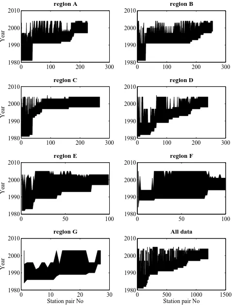
Fig. 1. Distribution of the time span for which the various station
pairs were sampled. The different panels shows the different geo-graphical areas (see Fig. 2). The time between the first and second repeat of a station are filled in, sorted by the time of the first cruise.
The Atlantic Ocean was divided into 7 areas in order to re-solve differences in the storage rate for different areas: (a) the western basin of the subpolar North Atlantic, (b) the eastern basin of the subpolar North Atlantic, (c) the western basin in the subtropical North Atlantic, (d) the eastern basin of the subtropical North Atlantic, (e) the tropical Atlantic between 15◦N/S, (f) the western basin of the South Atlantic, and (g) the eastern basin of the South Atlantic (e.g. Fig. 2). No dis-tinction was made between subpolar and subtropical South Atlantic due to limited number of data in the South Atlantic, but due regional differences in storage rates we sub-divided regions A and B into a northern and southern part. The station pairs that we have used for the calculation of storage rates are unevenly distributed through the regions, potentially causing spatial bias in estimates of average storage rates. In order to reduce the biasing effects, we divided the Atlantic in 2◦×2◦ bins (separated by odd latitudes and even longitudes), cal-culated the arithmetic mean of the storage rates in each bin, and finally averaged the bins in order to calculate the average storage rate for the regions. The mean storage rates for each bin were used to calculate the 95 % confidence interval (CI) of the mean (Table 1). Bins with no data were not included in
the calculation of average storage rates or confidence inter-vals, i.e. we did not attempt to interpolate our data to cover areas without any data, see Sect. 2.3 for a discussion on po-tential biases.
2.3 Sources of uncertainties
We now consider several sources of uncertainty in the storage rate estimates related to either: (1) the calculation of storage rates for a station pair, or (2) for calculating average storage rates (and their uncertainty) for a region; these will be dis-cussed separately below.
2.3.1 Uncertainty in storage rate for a station pair
Table 1. Averaged storage rates of DIC, DICabio, Oxygen and AOU for the 7 regions (see Figs. 2–5) and for the whole Atlantic as described in the text. The top row of each cell gives the average storage rates of the 2◦×2◦bins within each region; the bottom line in each cell gives the 95 % confidence interval. The number of samples (i.e. station pairs,N) for each area is indicated in the left column.
Region DIC DICabio Oxygen AOU
mol m−2yr−1 mol m−2yr−1 mol m−2yr−1 mol m−2yr−1
A – subpolar NW 0.97 0.63 −0.80 0.49
N=226 0.62–1.31 0.15–1.12 −1.36 –(−0.23) 0.13–0.85
A – north 0.57 −0.07 −1.67 0.96
N=201 0.15–0.99 −0.58–0.43 −2.20–(−1.15) 0.56–1.35
A – south 1.43 1.47 0.12 −0.05
N=25 0.95–1.91 0.89–2.05 −0.46–0.91 −0.57–0.45
B – subpolar NE 0.91 0.40 −0.94 0.78
N=256 0.63–1.19 0.06–0.73 −1.39–(−0.48) 0.45–1.12
B – North 0.44 −0.42 −1.96 1.29
N=166 −0.04–0.92 −0.84–0.00 −2.61–(−1.31) 0.73–1.85
B – South 1.12 0.77 −0.47 0.56
N=90 0.80–1.45 0.42–1.11 −0.96–0.01 0.15–0.97
C – subtropical NW 0.91 0.77 −0.12 0.19
N=267 0.63–1.20 0.46–1.08 −0.63–0.39 −0.15–0.53
D – subtropical NE 0.89 0.79 −0.08 0.07
N=240 0.66–1.12 0.54–1.04 −0.37–0.22 −0.26–0.39
E – tropics 0.35 0.56 0.30 −0.28
N=99 0.00–0.69 0.23–0.88 −0.08–0.68 −0.66–0.10
F – SW Atlantic 0.30 0.32 0.00 −0.02
N=100 −0.20–0.80 −0.07–0.70 −0.28–0.28 −0.36–0.32
G – SE Atlantic 1.98 2.04 −0.32 0.01
N=27 1.38–2.60 1.47–2.61 −0.70–0.06 −0.30–0.33
The whole Atlantic 0.86 0.73 −0.24 0.18
N=1204 0.72–1.00 0.59–0.87 −0.41–(−0.07) 0.04–0.32
0.8 mol m−2(assuming the samples above and below are ac-curate).
2.3.2 Uncertainty in the storage rate for a region
In this study, we are comparing pointwise changes in col-umn inventories which means that we are sensitive to ocean variability such as eddies, shifts in fronts and water masses in our analysis. If these shifts are happening on short time scales they can bias the analysis, but if they are more per-manent shifts in water mass distribution, etc. they represent changes that we do want to explore in this study. Our ap-proach involves two-point comparisons at many locations and for many different time intervals, and thereby involves both temporal and spatial averaging. In fact, one difficulty in presenting the storage rates is that the station pairs cover both different time spans and regions. The confidence inter-vals presented in this study are based solely on the storage rates for 2◦×2◦bins that have been sampled. However, large
areas of the Atlantic Ocean do not have any data (e.g. Fig. 2) so that there is a distinct possibility that our average values are biased in either direction. The samples are clearly not ran-domly distributed (both in time and space), making it difficult to assign rigorous confidence limits. The magnitude of these potential biases is difficult to assess, but it is safe to assume that the confidence intervals we present are lower limits. Fig-ures 2–6 and 11 present the storage rates for all station pairs and illustrate the spatial and temporal variability in storage rates.
3 Results
−2 −1.5 −1 −0.5 0 0.5 1 1.5 2 2.5 3
DIC storage rate [mol m−2 year−1] DIC storage rate
80oW 60o 40o 20o 0o 20oE 50oS
25o 0o 25o 50oN
A B
C D
E
F G
−20 0 2 50
100
whole Atlantic
[mol m−2 year−1] 0
2 4
Region A
0 2
4 0
2 4
Region B
0 5 10
0 10 20
Region C
0 10 20
Region D
0 5 10
Region E
0 5 10
Region F
−20 0 2 2
4 6
Region G
[image:7.595.129.469.65.344.2][mol m−2 year−1]
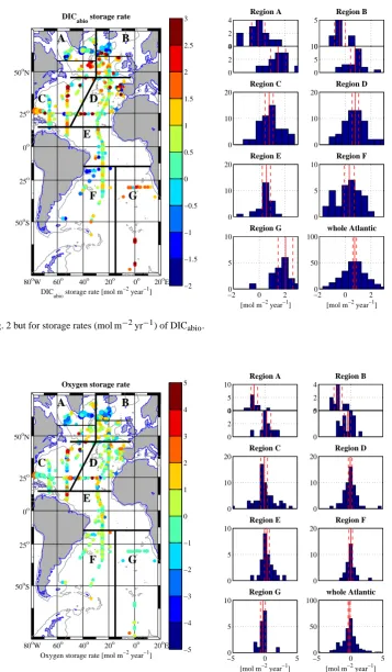
Fig. 2. Change in column inventory between two repeats of the same position, i.e. the storage rate (mol m−2yr−1) for DIC in the Atlantic Ocean. Left side panel: the average of storage rates for each location is shown with the color-coded marker; the sizes of the markers are made proportionally larger depending on the number of repeats at each position. The 2000 m isobath is marked with a gray thin line. Right hand panels: histograms of the distribution of storage rates in 2◦×2◦bins (see text) for the 7 regions and for the sum of all the regions; note that for regions A and B, we show the southern (lower panel) and northern (upper panel) sub-regions separately (thin black lines on the map). The average value and the 95 % confidence intervals are marked with red vertical lines.
vertical resolution to make meaningful vertical interpolation of the profiles. The insufficient vertical resolution for sev-eral of the profiles (particularly in the upper ocean) will most likely also affect attempts to interpolate any property over the entire basin for calculating inventories of, for instance, an-thropogenic carbon. The storage rates and CIs for all regions and variables are listed in Table 1 and graphical represen-tations of the spatial distribution of storage rates are shown in Figs. 2–5. In these figures all data that pass the criteria for a valid repeat measurement mentioned above are plotted; bluish colors for decreasing and green or reddish colors for increasing column inventories. Figure 6 represent the con-densed information from Figs. 2–5, also listed in Table 1. A different view of the distribution of the storage rates is pro-vided by the histograms in the right hand panel of Figs. 2–5, where the 95 % confidence interval and the mean are indi-cated with vertical red lines.
It is evident from the maps in Figs. 2–5 that a bipolar dis-tribution, i.e. non-Gaussian, of storage rates is present in sev-eral regions. Particularly, the northern parts of regions A and B in the SPNA (i.e. the Irminger, Labrador, and northern Ice-land Seas) are different from the southern parts of those re-gions. This is reflecting regional differences in storage rates,
and will be discussed in more detail below. We are therefore presenting the average storage rates and confidence intervals for the northern and southern parts of regions A and B sepa-rately.
3.1 DIC and DICabiostorage rates
−2 −1.5 −1 −0.5 0 0.5 1 1.5 2 2.5 3
DIC
abio storage rate [mol m −2 year−1] DIC
abio storage rate
80oW 60o 40o 20o 0o 20oE 50oS
25o 0o 25o 50oN
A B
C D
E
F G
−20 0 2 50
100
whole Atlantic
[mol m−2 year−1] 0
2 4
Region A
0 2
4 0
5
Region B
0 5 10
0 10 20
Region C
0 10 20
Region D
0 10 20
Region E
0 5 10
Region F
−20 0 2 5
10
Region G
[image:8.595.115.473.69.682.2][mol m−2 year−1]
Fig. 3. Same as Fig. 2 but for storage rates (mol m−2yr−1) of DICabio.
−5 −4 −3 −2 −1 0 1 2 3 4 5
Oxygen storage rate [mol m−2 year−1] Oxygen storage rate
80oW 60o 40o 20o 0o 20oE 50oS
25o 0o 25o 50oN
A B
C D
E
F G
−50 0 5 50
100
whole Atlantic
[mol m−2 year−1] 0
5 10
Region A
0 2
4 0
2 4
Region B
0 5
0 10 20
Region C
0 10 20
Region D
0 5 10
Region E
0 10 20
Region F
−50 0 5 5
10
Region G
[image:8.595.130.298.78.339.2][mol m−2 year−1]
−3 −2.5 −2 −1.5 −1 −0.5 0 0.5 1 1.5 2 2.5 3
AOU storage rate [mol m−2 year−1] AOU storage rate
80oW 60o 40o 20o 0o 20oE 50oS
25o 0o 25o 50oN
A B
C D
E
F G
−2 0 2 0
50 100
whole Atlantic
[mol m−2 year−1] 0
2 4
Region A
0
5 0
2 4
Region B
0 5 10
0 5 10 15
Region C
0 5 10 15
Region D
0 5 10
Region E
0 5 10 15
Region F
−2 0 2 0
5 10
Region G
[image:9.595.130.299.69.327.2][mol m−2 year−1]
Fig. 5. Same as Fig. 2 but for storage rates (mol m−2yr−1) of AOU.
A−n B−n A−s B−s C D E F G All −3
−2 −1 0 1 2 3
Regions
storage rate [mol m
−2 y −1]
Storage Rates
DIC DICabio oxygen −AOU
Fig. 6. Graphical representation of the storage rates for DIC,
DICabio, oxygen and AOU for the 9 regions (regions C–G and the northern and southern sub-regions for A and B) as well as the whole Atlantic Ocean. The vertical error bars represent the 95 % confi-dence interval of the data.
The averaged DIC and DICabiostorage rates for the north-ern North Atlantic (regions A and B) are generally some-what smaller (Table 1) than reported storage rates of anthro-pogenic carbon in this area (e.g. Sabine and Tanhua, 2010).
Perfect agreement is not expected, however, because other published methods tend to implicitly correct for changes DIC caused by biological activity and circulation in order to cal-culate the “anthropogenic carbon”, see Sect. 4, below. An-other obvious reason for these differences is that our method only evaluates the changes in the water column above 2000 m depth, whereas the published literature generally analyzes the whole water column. For the North Atlantic a significant amount of anthropogenic carbon has penetrated the water column deeper than 2000 m depth (e.g. Tanhua et al., 2007; Sabine and Tanhua, 2010; P´erez et al., 2010). This bias can probably be up to about 0.5 mol m−2yr−1, but must vary spa-tially depending on the presence of recently ventilated deep water. There are also significant differences in storage rates DIC and DICabiobetween the northern and southern parts of regions A and B (Figs. 2 and 3); the storage rates are gen-erally higher in the south and for stations pairs with a large time span (i.e. time between repeats). The DICabio storage rates are lower than the DIC storage rates for regions A and B, see Sect. 3.
[image:9.595.49.288.387.582.2]rates are found by Tanhua et al. (2007), see also Sabine and Tanhua (2010). The tropical region (region E) has relatively low storage rates of DIC and DICabio(Table 1), in agreement with the low inventory of Cant(e.g. Lee et al., 2003) in the tropical Atlantic, although significant spatial variability has been noted for the tropical Atlantic (Schneider et al., 2012).
In the southwest Atlantic (region F) we find stor-age rates of DIC and DICabio insignificantly larger than the “no change” condition, i.e. the storage rates are in-significantly different from zero, Table 1. However, (Wan-ninkhof et al., 2010) found find high storage rates of Cant (0.76 mol m−2yr−1) in the Southwest Atlantic along the WOCE section A16, i.e. in region F. Similarly, R´ıos et al. (2012) also finds high (0.92±0.13 mol m−2yr−1) stor-age rates of Cant for the southwest Atlantic Ocean. For the southeast Atlantic, region G in Fig. 1, we find the highest inventory rate of DIC and DICabioof all our areas in the At-lantic (Table 1). This is in contrast to the results presented by Murata et al. (2008) who found an inventory rate of only 0.43–0.49 mol m−2yr−1, (although for Cant) partly using the same data as in this study (i.e. the repeats of WOCE section A10 in 1993 and 2003). Note that the previously published results are assessing the change in Cant, so that a difference can be expected.
The well-known pattern of Cant column inventory, i.e. high values in the subpolar North Atlantic (SPNA), low in the tropics and intermediate values in the subtropics of both hemispheres, are not well reflected in our maps of DIC and DICabiostorage rates (Figs. 2 and 3). Interestingly, we find relatively low DICabiostorage rates in the subpolar North Atlantic, a region where large positive storage rates have been reported for Cant (e.g. Friis et al., 2005; P´erez et al., 2008, 2010). The difference between storage rates of DIC and DICabio in this region would be even large if we adopt the higher C/-O2 ratio of K¨ortzinger et al. (2001), i.e. the DICabio storage rate for region A-north would be
−0.15 mol m−2yr−1rather than−0.07 mol m−2yr−1. In this data set, there are signs of higher than average increase of DIC and DICabiooff the Iberian Peninsula, in the southeast Atlantic, off Florida and close to the Charlie-Gibbs Fracture Zone, and possibly in the northwest subtropical Atlantic.
4 Oxygen and AOU storage rates
For oxygen and AOU a somewhat different picture emerges (Figs. 4 and 5). For the Atlantic Ocean as a whole there is a negative storage rate of oxygen; the average of all our data is−0.24 (CI:−0.41–(−0.07)) mol m−2yr−1, and a positive storage rate of AOU; 0.18 (CI: 0.004–0.32) mol m−2yr−1. The storage rates of oxygen and AOU are significantly dif-ferent from zero for regions A and B only, as well for the average over all regions. Particularly, significant decrease in oxygen (and increase in AOU) column inventories are ob-served in the Labrador Sea, the Irminger Sea and in the
north-ern part of the Iceland Basin. The change in AOU, and the confidence interval of the change, is somewhat smaller than that for oxygen indicting that some of variability is tied to changes in solubility, mostly due to changes in temperature of the water. This solubility component of the O2 changes must be closely tied to the change in the inventory of heat. For instance, out-gassing of oxygen due to a warming ocean will not cause any direct changes in AOU, i.e. changes in AOU are indicative of air-sea O2fluxes driven by biology or circulation. For the regions outside of SPNA, no significant change in the column inventory of oxygen or AOU can be detected with this method.
4.1 Temporal variations
In order to identify any temporal trends in storage rates, the data on storage rates for three different time periods are evaluated. Station pairs where both repeats are conducted in the any of the time-periods 1980–1995, 1990–2000, or 1995–2005 were identified. This required discarding addi-tional pairs done more than 15 (or 10) yr apart, which further increases the uncertainty of the storage rates for each area (i.e. decreases the number of available samples). Since the resulting coverage is very sparse in most regions, we focus on the two northernmost regions (A – the western part of the SPNA, and B – the eastern portion of the SPNA) where more data is available, and where significant changes in deep wa-ter formation has occurred over time (e.g. Rhein et al., 2011). The data for the 3 time periods are displayed in Figs. 7 to 10 for DIC, DICabio, oxygen and AOU, respectively. In Fig. 11 the information for regions A and B is condensed.
It can be noted that, as expected, significant spatial vari-ations are present, even within each region, but that some interesting patterns can be recognized. For the first time slice (1980–1995) an increase in oxygen, DIC and DICabiocan be observed for both regions (i.e. positive storage rates), partic-ular for region B, although only a limited number of station pairs are available to confirm this trend. During the1990s the conditions are significantly different with negative storage rates of oxygen and close to neutral storage rates of DIC. During the last time slice (1995–2005) again a different pic-ture emerges with different patterns for the western and the eastern domain. For region A, the storage rate for oxygen is continuously negative whereas the DIC positive; region B show positive storage rates of DIC but neutral oxygen storage rates. It is clear that there are both temporal and spatial vari-ability in the storage rates of DIC and oxygen in the North Atlantic subpolar gyre, particularly for the northern part of the region.
5 Discussion
−2 −1.5 −1 −0.5 0 0.5 1 1.5 2 2.5 3
DIC [mol m−2 year−1] 1995 − 2005 repeats
75oW 60o 45o 30o 15o 0o 18oS
0o 18o 36o 54oN
A B
C D
E
DIC [mol m−2 year−1] 1990 − 2000 repeats
75oW 60o 45o 30o 15o 0o 18oS
0o 18o 36o 54oN
A B
C D
E
DIC [mol m−2 year−1] 1980 − 1995 repeats
75oW 60o 45o 30o 15o 0o 18oS
0o 18o 36o 54oN
A B
C D
[image:11.595.113.484.63.225.2]E
Fig. 7. Storage rates for DIC for three different time periods. Left panel – storage rates for repeats where both cruises were conducted between
1980 and 1995; middle panel – both repeats were conducted between 1990 and 2000; right panel – both repeats were conducted between 1995 and 2005. The 2000 m isobath is marked with a gray thin line.
DICabio [mol m−2 year−1] 1990 − 2000 repeats
75oW 60o 45o 30o 15o 0o 18oS
0o 18o 36o 54oN
A B
C D
E
DICabio [mol m−2 year−1] 1980 − 1995 repeats
75oW 60o 45o 30o 15o 0o 18oS
0o 18o 36o 54oN
A B
C D
E
−2 −1.5 −1 −0.5 0 0.5 1 1.5 2 2.5 3
DICabio [mol m−2 year−1] 1995 − 2005 repeats
75oW 60o 45o 30o 15o 0o 18oS
0o 18o 36o 54oN
A B
C D
E
Fig. 8. Same as Fig. 7 but for storage rates (mol m−2a−1) of DICabio.
Canthas been increasing from roughly 0.2 mol m−2yr−1 in 1960 to 0.6 mol m−2yr−1in 2007 (Khatiwala et al., 2009). The storage rate is expected to show significant regional variability assuming that the regional pattern of storage rate is similar to that of the total storage, see for instance the Atlantic Ocean map of Cant column inventory in Lee et al. (2003). However, there are a few important differences between this study and the calculation by Lee et al. (2003). Most importantly this study reports on the change in DIC and DICabiowhich is not equal to the change in Cantso that temporal changes in the storage rate of DIC which is not evi-dent by observing the total storage of Cantbecomes relevant. Changes in DICabioshould be largely conserved in the ocean interior as it compensates for respiration, but could change in surface water due to either air–sea exchange of CO2 or O2. Changes in column inventory of DICabiowill therefore largely reflect a combination of the effects of long-term CO2 and O2exchange with the atmosphere, with the CO2 effect presumably dominating as a result of the uptake of
anthro-pogenic CO2. The regional patterns of storage rate of DIC and DICabioin this analysis is significantly different than the well-known distribution of column inventory of Cantin the Atlantic Ocean. In general, a mixed pattern of positive and negative storage rates are found in each region. The picture generally gets somewhat less patchy when considering only shorter time-periods, Figs. 6–9. Since this method of calcu-lating storage rates does not account for small-scale temporal and spatial variability due to, for instance eddies and move-ments of oceanic fronts, larger variability in the storage rate is expected than from methods that do compensate for this, such as MLR based approaches. The larger scatter also reflect the additional difficulties in determining inventory changes for the total amount of DIC rather than the anthropogenic perturbation (Cant), see discussion below.
[image:11.595.114.481.283.448.2]−5 −4 −3 −2 −1 0 1 2 3 4 5
Oxygen [mol m−2 year−1] 1995 − 2005 repeats
75oW 60o 45o 30o 15o 0o 18oS
0o 18o 36o 54oN
A B
C D
E
Oxygen [mol m−2 year−1] 1990 − 2000 repeats
75oW 60o 45o 30o 15o 0o 18oS
0o 18o 36o 54oN
A B
C D
E
Oxygen [mol m−2 year−1] 1980 − 1995 repeats
75oW 60o 45o 30o 15o 0o 18oS
0o 18o 36o 54oN
A B
C D
[image:12.595.113.479.64.229.2]E
Fig. 9. Same as Fig. 7 but for storage rates (mol m−2a−1) of oxygen.
AOU [mol m−2 year−1] 1980 − 1995 repeats
75oW 60o 45o 30o 15o 0o 18oS
0o 18o 36o 54oN
A B
C D
E
AOU [mol m−2 year−1] 1990 − 2000 repeats
75oW 60o 45o 30o 15o 0o 18oS
0o 18o 36o 54oN
A B
C D
E
−3 −2.5 −2 −1.5 −1 −0.5 0 0.5 1 1.5 2 2.5 3
AOU [mol m−2 year−1] 1995 − 2005 repeats
75oW 60o 45o 30o 15o 0o 18oS
0o 18o 36o 54oN
A B
C D
E
Fig. 10. Same as Fig. 7 but for storage rates (mol m−2a−1) of AOU.
based on transient tracer observations. This is roughly the same time period (1995–2005) for which we find a signif-icant increase in the column inventory of DIC and DICabio storage rates in the same region. A water mass analysis sug-gest that the volume of the classic Labrador Sea Water (LSW) decreased due to decreasing deep water formation in the Labrador Sea, and as a consequence there is an increase of a lighter (i.e. less dense) version of the LSW (e.g. Rhein et al., 2011; Steinfeldt et al., 2009). Thus the deep version of the LSW only experience limited ventilation during this time, i.e. the LSW is getting “older”. This provides an expla-nation to the observation that the column inventory of Cant remains close to constant (restricted communication with the increasing atmospheric CO2concentrations) and why the DIC is increasing (remineralization of organic matter) more than DICabio and oxygen concentrations decreases during this time period. This analysis thus confirms the conclusion by Steinfeldt et al. (2009) that the northwest subpolar gyre of the Atlantic Ocean is a region that shows significant
devia-tion from the expected average uptake rate of anthropogenic carbon.
[image:12.595.114.480.260.427.2]1980−1995 1990−2000 1995−2005 −4
−3 −2 −1 0 1 2 3 4
storage rate [mol m
−2
y
−1]
Region A
DIC DIC abio oxygen −AOU
1980−1995 1990−2000 1995−2005 Region B
[image:13.595.52.286.65.183.2]DIC DIC abio oxygen −AOU
Fig. 11. Storage rates for DIC, DICabio, AOU and oxygen for re-gions A and B for three time periods (1980–1995, 1990–2000, and 1995–2005), see Figs. 6–9. Note that negative AOU is plotted and that the markers are slightly offset for clarity. The error-bars the 95 % confidence interval of the variation of storage rates within each area calculated from the values of the 2◦×2◦bins (see text).
correlate this to the North Atlantic Oscillation (NAO) and the formation rate of Labrador Sea Water. They find particularly high storage rates during the period 1991 to 1998 (i.e. during the time of intense formation of LSW) for the Irminger Sea and the Iceland Basin, whereas the East North Atlantic Basin seem to have a more linear increase of storage rate for Cant (0.77±0.03 mol m−2yr−1) (P´erez et al., 2008, 2010). This overlaps with the time period (1990–2000) where we find slightly negative storage rates for DIC and DICabio. However, since the analysis in this study is only covering the upper 2000 m of the water column, storage changes in the deeper part of the water column remains unaccounted for. For this region, with active deep water formation and significant ad-vection of overflow water, the deeper parts might indeed be important and is a source of error in this comparison. Signif-icant temporal variations inT,Sand dissolved O2occurred in the SPNA during the last∼60 yr are also reported by van Aken et al. (2011) who conclude that the long-term varia-tions of the intermediate water mass properties in the SPNA are related to meteorological forcing of the Labrador Sea. Significant changes in the SPNA salinity balance has been observed during the last half century (Curry and Mauritzen, 2005) which can be consistent with varying dominance of different water masses. Based on this analysis it seems that these long-term variations also affect the inventory of DIC in the SPNA.
The storage rates of DIC and DICabio in the southern parts of regions A and B are significantly higher than for the north-ern parts, and conform better to published estimates of Cant in the region. For instance, a recent study by McGrath et al. (2012) found storage rates of Cantin the Rockall Trough of 1.2 mol m−2a−1 for the layer between 200 and 2000 m. The oxygen and AOU storage rates are close to neutral in the southern parts of regions A and B, i.e. similar to other areas further south in the Atlantic.
A detailed study of the temporal evolution of the inorganic carbon content in the SPNA is out of scope for this study. It is, however, interesting to point out the diverging trends of Cantand DIC found in this region may relate to varying con-vection activity and water mass distribution. It seems that the inventory of DIC decreases at the same time as the inven-tory of Cant increases. An explanation for this can be pro-vided by changes in water mass distribution in the SPNA. For instance, the DIC concentration of LSW is in the order of 2160 µmol kg−1, whereas the DIC concentration of the Mediterranean Sea Overflow Water (in the Gulf of Cadiz) is in the order of 2200 µmol kg−1, even though both water masses have relatively high, and somewhat similar concen-tration of Cant. These two water masses are both present in the SPNA and variability in the relative presence of these two water masses will change the column inventory of DIC in a way that is not necessarily reflected in storage of Cant.
Recently, Stendardo and Gruber (2012) used a long-term data set for dissolved oxygen in the North Atlantic Ocean to assess any trends over the past 49 yr. She finds a complex pattern of temporal changes in oxygen concentrations; the upper water masses have generally lost oxygen, particularly in the eastern and northern Atlantic, whereas deeper layers have generally gained oxygen, particularly in the southwest-ern part of the North Atlantic. The results are based on ob-served changes in oxygen concentration for different density intervals (i.e. water masses). In a more detailed study focus-ing of repeats of the A2 sections (i.e. a zonal section across the Atlantic Ocean at∼47◦N), Stendardo (2011) concludes that the oxygen concentrations show strong inter-annual vari-ability with a tendency towards oxygen loss over time. The results presented in this study are, in general, supporting the results of Stendardo (2011) with particularly large losses of oxygen in the northern part of the North Atlantic. However, the results are difficult to compare direct as this study is fo-cusing on the changes in column inventory rather than the concentration in various water masses.
6 Concluding remarks
in the ocean. One important aspect of this analysis is that variations in water mass prevalence have a large influence on inventories of interior ocean properties so that the total DIC inventory can decrease in an area even if the inventory of Cantsignificantly increases. This has implications for bal-ancing the global carbon budget that do not distinguish be-tween “anthropogenic carbon” and “natural carbon”. From a global perspective it is the overall increasing or decreasing inventory of carbon in the ocean that matters to balance the budget.
Acknowledgements. The research leading to these results was supported through EU FP7 project CARBOCHANGE “Changes in carbon uptake and emissions by oceans in a changing climate” which received funding from the European Community’s Seventh Framework Programme under grant agreement no. 264879. We thank Mark Lenz for useful discussions on statistics. This work was carried out in part while RFK was on sabbatical leave at the Leibniz Institute of Marine Sciences in Kiel, supported by the Humboldt Foundation and the Cluster of Excellence “FutureOcean”.
Edited by: F. Joos
References
Anderson, L. A. and Sarmiento, J. L.: Redfield ratios of rem-ineralization determined by nutrient data analysis, Global Bio-geochem. Cy., 8, 65–80, 1994.
Cermeno, P., Dutkiewicz, S., Harris, R. P., Follows, M., Schofield, O., and Falkowski, P. G.: The role of nutricline depth in regulat-ing the ocean carbon cycle, P. Natl. Acad. Sci. USA, 105, 20344– 20349, doi:10.1073/pnas.0811302106, 2008.
Curry, R. and Mauritzen, C.: Dilution of the Northern North At-lantic Ocean in Recent Decades, Science, 308, 1772–1774, doi:10.1126/science.1109477, 2005.
Friis, K., K¨ortzinger, A., P¨atsch, J., and Wallace, D. W. R.: On the temporal increase of anthropogenic CO2 in the sub-polar North Atlantic, Deep-Sea Res. Part I, 52, 681–698, doi:10.1016/j.dsr.2004.11.017, 2005.
Gammon, R. H., Cline, J., and Wisegarver, D. P.: Chluorofluo-romethanes in the Northeast Pacific Ocean: Measured Verti-cal Distribution and Application as Transient Tracers of Upper Ocean Mixing, J. Geophys. Res., 87, 9441–9454, 1982. Helm, K. P., Bindoff, N. L., and Church, J. A.: Observed decreases
in oxygen content of the global ocean, Geophys. Res. Lett., 38, L23602, doi:10.1029/2011gl049513, 2011.
Keeling, R. F.: Comment on “The Ocean Sink for Anthropogenic CO2”, Science, 308, 1743c, 2005.
Keeling, R. F. and Garcia, H. E.: The change in oceanic O-2 inven-tory associated with recent global warming, P. Natl. Acad. Sci. USA, 99, 7848–7853, 2002.
Keeling, R. F., K¨ortzinger, A., and Gruber, N.: Ocean Deoxygena-tion in a Warming World, Annual Review of Marine Science, 2, 199–229, doi:10.1146/annurev.marine.010908.163855, 2010. Key, R. M., Kozyr, A., Sabine, C. L., Lee, K., Wanninkhof, R.,
Bullister, J. L., Feely, R. A., Millero, F. J., Mordy, C., and Peng, T. H.: A global ocean carbon climatology: Results from Global
Data Analysis Project (GLODAP), Global Biogeochem. Cy., 18, GB4031, doi:1029/2004GB002247, 2004.
Key, R. M., Tanhua, T., Olsen, A., Hoppema, M., Jutterstr¨om, S., Schirnick, C., van Heuven, S., Kozyr, A., Lin, X., Velo, A., Wal-lace, D. W. R., and Mintrop, L.: The CARINA data synthesis project: introduction and overview, Earth Syst. Sci. Data, 2, 105– 121, doi:10.5194/essd-2-105-2010, 2010.
Khatiwala, S., Primeau, F., and Hall, T.: Reconstruction of the his-tory of anthropogenic CO2concentrations in the ocean, Nature, 462, 346–349, doi:10.1038/nature08526, 2009.
K¨ortzinger, A., Hedges, J. I., and Quay, P. D.: Redfield ratios revis-ited: Removing the biasing effect of anthropogenic CO2, Limnol. Oceanogr., 46, 964–970, 2001.
Lee, K., Choi, S.-D., Park, G.-H., Wanninkhof, R., Peng, T. H., Key, R. M., Sabine, C. L., Feely, R. A., Bullister, J. L., Millero, F. J., and Kozyr, A.: An updated anthropogenic CO2 inven-tory in the Atlantic Ocean, Global Biogeochem. Cy., 17, 1116, doi:10.1029/2003GB002067, 2003.
Levine, N. M., Doney, S. C., Wanninkhof, R., Lindsay, K., and Fung, I. Y.: Impact of ocean carbon system variability on the de-tection of temporal increases in anthropogenic CO2, J. Geophys. Res., 113, C03019, doi:10.1029/2007JC004153, 2008.
Levitus, S., Antonov, J. I., Boyer, T. P., Baranova, O. K., Garcia, H. E., Locarnini, R. A., Mishonov, A. V., Reagan, J. R., Seidov, D., Yarosh, E. S., and Zweng, M. M.: World ocean heat content and thermosteric sea level change (0–2000 m), 1955–2010, Geophys. Res. Lett., 39, L10603, doi:10.1029/2012gl051106, 2012. McGrath, T., Kivim¨ae, C., Tanhua, T., Cave, R. R., and
Mc-Govern, E.: Inorganic carbon and pH levels in the Rock-all Trough 1991–2010, Deep-Sea Res. Part I, 68, 79–91, doi:10.1016/j.dsr.2012.05.011, 2012.
Murata, A., Kumamoto, Y., Sasaki, K., Watanabe, S., and Fuka-sawa, M.: Decadal increases of anthropogenic CO2in the sub-tropical South Atlantic Ocean along 30 degrees S, J. Geophys. Res., 113, C06007, doi:10.1029/2007JC004424, 2008.
Peng, T.-H. and Wanninkhof, R.: Increase in anthropogenic CO2in the Atlantic Ocean in the last two decades, Deep-Sea Res. Part I, 57, 755–770, doi:10.1016/j.dsr.2010.03.008, 2010.
P´erez, F. F., V´azquez-Rodr´ıguez, M., Louarn, E., Pad´ın, X. A., Mercier, H., and R´ıos, A. F.: Temporal variability of the an-thropogenic CO2storage in the Irminger Sea, Biogeosciences, 5, 1669–1679, doi:10.5194/bg-5-1669-2008, 2008.
P´erez, F. F., V´azquez-Rodr´ıguez, M., Mercier, H., Velo, A., Lher-minier, P., and R´ıos, A. F.: Trends of anthropogenic CO2storage in North Atlantic water masses, Biogeosciences, 7, 1789–1807, doi:10.5194/bg-7-1789-2010, 2010.
Pierrot, D., Brown, P., Van Heuven, S., Tanhua, T., Schuster, U., Wanninkhof, R., and Key, R. M.: CARINA TCO2 data in the Atlantic Ocean, Earth Syst. Sci. Data, 2, 177–187, doi:10.5194/essd-2-177-2010, 2010.
Rhein, M., Kieke, D., H¨uttl-Kabus, S., Roessler, A., Mertens, C., Meissner, R., Klein, B., B¨oning, C. W., and Yashayaev, I.: Deep water formation, the subpolar gyre, and the meridional overturn-ing circulation in the subpolar North Atlantic, Deep-Sea Res. Part II, 58, 1819–1832, doi:10.1016/j.dsr2.2010.10.061, 2011. Riebesell, U., Schulz, K. G., Bellerby, R. G. J., Botros, M.,
doi:10.1038/nature06267, 2007.
R´ıos, A. F., Velo, A., Pardo, P. C., Hoppema, M., and P´erez, F. F.: An update of anthropogenic CO2 storage rates in the western South Atlantic basin and the role of Antarctic Bottom Water, J. Mar. Systems, 94, 197–203, doi:10.1016/j.jmarsys.2011.11.023, 2012.
Sabine, C. L. and Tanhua, T.: Estimation of Anthropogenic CO2 Inventories in the Ocean, Annual Reviews of Marine Sciences, 2, 175–198, doi:10.1146/annurev-marine-120308-080947, 2010. Sabine, C. L., Key, R. M., Johnson, K. M., Millero, F. J., Pois-son, A., Sarmiento, J. L., Wallace, D. W. R., and Winn, C. D.: Anthropogenic CO2inventory of the Indian Ocean, Global Bio-geochem. Cy., 13, 179–198, 1999.
Sabine, C. L., Key, R. M., Kozyr, A., Feely, R. A., Wanninkhof, R., Millero, F., Peng, T. H., Bullister, J., and Lee, K.: Global Ocean data analysis project (GLODAP): Results and data, ORNL/CDIAC-145, NDP-083, 2005.
Schneider, A., Tanhua, T., K¨ortzinger, A., and Wallace, D. W. R.: An evaluation of tracer fields and anthropogenic car-bon in the equatorial and the tropical North Atlantic, Deep-Sea Res. Part I: Oceanographic Research Papers, 67, 85–97, doi:10.1016/j.dsr.2012.05.007, 2012.
Steinfeldt, R., Rhein, M., Bullister, J. L., and Tanhua, T.: Inven-tory changes in anthropogenic carbon from 1997–2003 in the At-lantic Ocean between 20 degrees S and 65 degrees N, Global Bio-geochem. Cy., 23, GB3010, doi:10.1029/2008GB003311, 2009. Stendardo, I.: Interannual to decadal variability and trends of the oceanic oxygen content in the North Atlantic, PhD, Institute of Biogeochemistry and Pollutant Dynamics, ETH, Z¨urich, 185 pp., 2011.
Stendardo, I., and Gruber, N.: Oxygen trends over five decades in the North Atlantic, J. Geophys. Res., 117, C11004, doi:10.1029/2012jc007909, 2012.
Stendardo, I., Gruber, N., and K¨ortzinger, A.: CARINA oxygen data in the Atlantic Ocean, Earth Syst. Sci. Data, 1, 87–100, doi:10.5194/essd-1-87-2009, 2009.
Tanhua, T. and Wallace, D. W. R.: Consistency of TTO-NAS Inor-ganic Carbon Data with modern measurements, Geophys. Res. Lett., 32, L14618, doi:10.1029/2005GL023248, 2005.
Tanhua, T., K¨ortzinger, A., Friis, K., Waugh, D. W., and Wallace, D. W. R.: An estimate of anthropogenic CO2inventory from decadal changes in ocean carbon content, P. Natl. Acad. Sci. USA., 104, 3037–3042, doi:10.1073/pnas.0606574104, 2007.
Tanhua, T., van Heuven, S., Key, R. M., Velo, A., Olsen, A., and Schirnick, C.: Quality control procedures and methods of the CARINA database, Earth Syst. Sci. Data, 2, 35–49, doi:10.5194/essd-2-35-2010, 2010.
Touratier, F. and Goyet, C.: Decadal evolution of anthropogenic CO2 in the northwestern Mediterranean Sea from the mid-1990s to the mid-2000s, Deep-Sea Res. Part I, 56, 1708–1716, doi:10.1016/j.dsr.2009.05.015, 2009.
Touratier, F., Azouzi, L., and Goyet, C.: CFC-11, Delta C-14 and H-3 tracers as a means to assess anthropogenic CO2concentrations in the ocean, Tellus B, 59, 318–325, 2007.
van Aken, H. M., Femke de Jong, M., and Yashayaev, I.: Decadal and multi-decadal variability of Labrador Sea Water in the north-western North Atlantic Ocean derived from tracer distributions: Heat budget, ventilation, and advection, Deep-Sea Res. Part I, 58, 505–523, doi:10.1016/j.dsr.2011.02.008, 2011.
Velo, A., Perez, F. F., Brown, P., Tanhua, T., Schuster, U., and Key, R. M.: CARINA alkalinity data in the Atlantic Ocean, Earth Syst. Sci. Data, 1, 45–61, doi:10.5194/essd-1-45-2009, 2009. Wakita, M., Watanabe, S., Murata, A., Tsurushima, N., and Honda,
M.: Decadal change of dissolved inorganic carbon in the sub-arctic western North Pacific Ocean, Tellus B, 62, 608–620, doi:10.1111/j.1600-0889.2010.00476.x, 2010.
Wanninkhof, R., Doney, S. C., Bullister, J. L., Levine, N. M., Warner, M., and Gruber, N.: Detecting anthropogenic CO2 changes in the interior Atlantic Ocean between 1989 and 2005, J. Geophys. Res., 115, C11028, doi:10.1029/2010JC006251, 2010. Weiss, R.: Solubility of Nitrogen, Oxygen and Argon in water and
seawater, Deep-Sea Res., 17, 721–735, 1970.