Geosci. Instrum. Method. Data Syst., 1, 103–109, 2012 www.geosci-instrum-method-data-syst.net/1/103/2012/ doi:10.5194/gi-1-103-2012
© Author(s) 2012. CC Attribution 3.0 License.
Geoscientific
InstrumentationMethods and
Data Systems
Discussions
Geoscientific
InstrumentationMethods and
Data Systems
Open
Access
Automatic parameterization for magnetometer zero offset
determination
M. A. Pudney1, C. M. Carr1, S. J. Schwartz1, and S. I. Howarth2
1The Blackett Laboratory, Imperial College London, London, SW7 2AZ, UK 2Astrium Ltd., Stevenage, SG1 2AS, UK
Correspondence to: M. A. Pudney ([email protected])
Received: 18 May 2012 – Published in Geosci. Instrum. Method. Data Syst. Discuss.: 13 June 2012 Revised: 10 August 2012 – Accepted: 21 August 2012 – Published: 30 August 2012
Abstract. In-situ magnetic field measurements are of crit-ical importance in understanding how the Sun creates and controls the heliosphere. To ensure the measurements are ac-curate, it is necessary to track the combined slowly varying spacecraft magnetic field and magnetometer zero offset – the systematic error in the sensor measurements. For a 3-axis sta-bilised spacecraft, in-flight correction of zero offsets primar-ily relies on the use of Alfv´enic rotations in the magnetic field. We present a method to automatically determine a key parameter related to the ambient compressional variance of the signal (which determines the selection criteria for identi-fying clear Alfv´enic rotations). We apply our method to dif-ferent solar wind conditions, performing a statistical analysis of the data periods required to achieve a 70 % chance of cal-culating an offset using Helios datasets. We find that 70 % of 40 min data periods in regions of fast solar wind possess sufficient rotational content to calculate an offset. To achieve the same 70 % calculation probability in regions of slow so-lar wind requires data periods of 2 h duration. We also find that 40 min data periods at perihelion compared to 1 h and 40 min data periods at aphelion are required to achieve the same 70 % calculation probability. We compare our method with previous work that uses a fixed parameter approach and demonstrate an improvement in the calculation probability of up to 10 % at aphelion and 5 % at perihelion.
1 Introduction
The magnetometer instrument is crucial to understanding coronal and solar wind acceleration, the heliospheric evo-lution over solar cycles, and the evoevo-lution of magnetic
structures, such as coronal mass ejections (Acu˜na, 2002). The instrument needs to be calibrated in order to obtain reli-able scientific data. Every magnetometer has a sensor offset, a systematic bias in a null field environment. Although this can be calibrated on the ground, after launch this bias will change (Balogh, 2010).
In addition to the sensor offset, there will be a magnetic field generated by the spacecraft (Acu˜na, 2002). The space-craft magnetic field consists of transient field jumps due to subsystem activities and a slowly varying residual field. The spacecraft induced transient fields, spacecraft induced resid-ual field and sensor offset need to be removed from the in-strument data in order to retrieve the ambient magnetic field for accurate scientific analysis (Acu˜na et al., 2008).
The dual magnetometer technique (first discussed by Ness et al., 1971) is designed to remove the transient spacecraft field jumps from the sensor data. This is achieved by mea-suring the magnetic field simultaneously using two spatially separated magnetometers, as used extensively on the Dou-ble Star (Carr et al., 2005) and Venus Express (Pope et al., 2011) missions. The ratio between the two sensor field read-ings will be unity for ambient field changes, and non-unity for spacecraft field changes, assuming that the ambient field is constant over the spatial distance between the two sensors (Pope et al., 2011).
This zero offset can be measured through a rotation of the spacecraft, assuming that the solar wind magnetic field mag-nitude and direction remain constant over the rotation period (Acu˜na et al., 2008). If a difference is detected in the mea-sured field magnitude between two or more samples of the same field, a vector zero offset is present and can be calcu-lated (Acu˜na, 2002). This method is effective for the spin-plane components of a permanently spinning spacecraft or for data taken during spacecraft roll manoeuvres (Kepko et al., 1996).
For a three-axis stabilised spacecraft, or the remaining axis of a spinning spacecraft (perpendicular to the spin plane), the most reliable way to regularly determine zero offsets is by us-ing pre-existus-ing Alfv´enic rotations in the solar wind – the so-lar wind variance method (Leinweber et al., 2008). The exis-tence of a zero offset along one field component will cause an artificial compression: a change in the measured field magni-tude correlated with a change in that component. Assuming the solar wind dataset is Alfv´enic, these artificial compres-sions can be attributed to a zero offset and removed, because Alfv´enic rotations are non-compressional – they do not affect the magnetic field magnitude (Kivelson, 1995). Therefore, ambient field component fluctuations should be uncorrelated with changes in the ambient field magnitude.
Davis and Smith (1968) were the first to take advantage of the Alfv´enic properties of the solar wind for zero offset calculation. They used a statistical technique that looks for the correlation between changes in a measured field compo-nent and changes in the square of the measured field magni-tude. The subsequent Belcher (1973) and Hedgecock (1975) methods are variants of the Davis-Smith method. However, all three methods are based on the same assumption that the solar wind fluctuations have a high Alfv´enicity – they are predominantly Alfv´enic – and therefore do not greatly affect the field magnitude.
However, the ambient magnetic field is never purely ro-tational. In reality, the ambient field contains both compres-sions and rotations, with relative contributions that depend on the heliospheric environment. It is therefore necessary to only select datasets in which the assumption of a high Alfv´enicity is sufficiently valid. This is achieved by a proce-dure developed by Leinweber et al. (2008) and summarised in Sect. 3. Leinweber et al. (2008) compared the three afore-mentioned solar wind variance methods and concluded that the optimum approach is to use the Davis and Smith (1968) method, with the addition of a number of checks to ensure that the dataset contains sufficient rotational content and min-imum compressional content. Such checks are referred to as “selection criteria” by Leinweber et al. (2008).
The Leinweber et al. (2008) procedure requires the speci-fication of multiple parameters, which they do on an empiri-cal basis for particular datasets. Leinweber et al. (2008) have chosen their selection criteria such that only one key param-eter needs to vary – the minimum compressional standard deviation (MCS). MCS is defined as the standard deviation
of the estimated ambient magnetic field magnitude over 1 h. MCS acts as a threshold, such that standard deviations over a lesser time period that are smaller than MCS can be assumed Alfv´enic. In order to track varying offsets systematically and with minimal human intervention, we extend the Leinweber et al. (2008) procedure by automatically determining MCS from the dataset.
The structure of this paper is as follows. First, we discuss the implementation of the solar wind variance method. Sec-ondly, we describe the algorithm used by Leinweber et al. (2008), including the use of selection criteria and the param-eter MCS. We then explain how our method automatically evaluates MCS from a given dataset. Using data from He-lios 2, we then go on to show what impact the solar wind conditions have on the probability at which offsets can be calculated using this new method. Finally, we compare our new method with previous work that keeps MCS constant.
2 The solar wind variance method
Assuming that the solar wind is purely Alfv´enic over a pe-riod of data, the existence of rotations in the ambient field can be used to find the zero offsets. The Davis and Smith (1968) method looks for the correlation between changes in a measured field component and changes in the square of the measured field magnitude. This is achieved by adding an unknown offset along each of the field components and then calculating the sample covariance between the measured field component variations and variations in the square of the measured field magnitude. Due to the assumption of pure Alfv´enicity, the covariance is set to equal zero, which allows the offsets to be calculated. Therefore, any correlation that is found to exist is attributed to a zero offset in this way. In order to solve offsets for all three axes, significant rotations around two or more axes are required.
However, the solar wind is never perfectly Alfv´enic – it contains ambient compressions and rotations – and it is im-possible to directly distinguish ambient field compressions from artificial compressions due to offsets. The best ap-proach is uses a subset of the original dataset where the as-sumption of high Alfv´enicity is close to being valid. By per-forming the Davis and Smith (1968) method on this subset, the resulting offset calculation will be much more reliable than if it were performed on the entire original dataset. This is the approach taken by Leinweber et al. (2008) in the next section, who use a windowing technique with selection crite-ria to choose the data subset.
3 The Leinweber et al. algorithm
3.1 Methodology
The Leinweber et al. (2008) algorithm uses variable win-dow sizes to identify non-compressive field rotations within a data period (see Fig. 1). The smallest window size (typically 5 min) is stepped forward by the step length (typically 8 s) until the end of the data period. This process is repeated with larger window sizes (increasing in length by 20 % each time) until the maximum window size has been reached, which is limited by the size of the data period. Each window passes or fails according to selection criteria, passing only those win-dows that contain sufficient rotational content and minimum levels of compression (see Sect. 3.2). A check is made to ensure that a sufficient number of windows are passed for use in the final offset calculation. The final offsets are then solved using the Davis and Smith (1968) method, now using the most rotational and least compressible content, namely the data from those windows that passed.
3.2 Selection criteria
For each individual data window, the Leinweber et al. (2008) algorithm performs the following steps:
1. The Davis and Smith (1968) method is performed to es-timate the offsets.
2. A first selection criterion is applied, which is designed to find magnetic field rotations. The criterion passes windows in which magnetic field fluctuations spanning at least a single plane are greater than the empirically chosen value MCS (see Sect. 3.3). Windows with fluc-tuations in only one component (i.e. linear) would indi-cate a compression and are therefore rejected.
3. The initial estimated offsets from step 1 are removed from the data to retrieve estimated ambient field com-ponents, from which the estimated ambient field magni-tude is calculated.
4. A second selection criterion is applied, which is de-signed to test whether the window has overall low lev-els of compression. The criterion compares the size of the component fluctuations to the field magnitude vari-ation and calculates the ratio between the two. Only ra-tios that stay above a fixed empirically determined value are passed.
5. A third selection criterion is applied, which only passes windows containing individual component variations that do not strongly correlate with variations in the recalculated magnitude – to within the MCS (see Sect. 3.3). This check is more rigorous than the first two, since it is applied to each individual field component in turn.
Fig. 1. An illustration of the time series nomenclature used in this
paper. The total data length is the complete set of data within a sin-gle data file, shown here to be 4 h. The data period is the dataset over which a final offset is calculated, shown here to be 1 h. Conse-quently, this total data length would provide four offset calculations. The data period is repeatedly sub-divided into the variable window sizes from a length of 5 min up to the maximum window size, which is equivalent to the data period.
3.3 The minimum compressional standard deviation
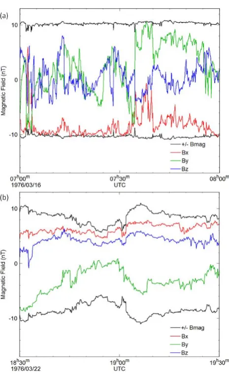
Fig. 2. (a) An example of an hour of incompressive rotation in the
solar wind (Helios 2). The black line, which remains relatively con-stant at 10nT, is the magnetic field magnitude and its negative. The components fluctuate strongly, indicating the presence of significant rotations. (b) An example of an hour of magnetic field variations that are naturally contaminated by compressions (Helios 2). Here the component variations are correlated with changes in the field magnitude, indicating strong compressional content.
4 Parameterizing the minimum compressional standard deviation
The choice of a value for MCS is a compromise between en-suring that a sufficient number of data windows are passed to allow an offset determination to be made and keeping the data in each window that passes the selection criteria as in-compressible as possible. Since the second selection crite-rion (which does not depend on MCS) rejects windows with high compressional content from the final offset calculation, it would seem to be better to ensure more data windows pass through the first selection criterion (Leinweber et al., 2008). If MCS is too large, windows will be less likely to pass the
first criterion, since the component variations will be consid-ered too small. However, if MCS is too small, windows will be less likely to pass the third criterion, since even small am-bient compressions will be considered unacceptable.
Since we do not know a priori what the correct value of MCS is, we use the standard deviation of the estimated field magnitude, as calculated in the procedure below, to parame-terize MCS. We find that this choice of MCS closely tracks the region of maximum passed windows. For a given data in-terval (the total data length) where magnetic field zero offsets need to be calculated, our procedure works as follows:
1. We choose the size of the data period and take a win-dow of data of that period from the start of the total data length.
2. We apply the Davis and Smith (1968) method to obtain an estimate for the offsets.
3. We subtract the estimated offsets from the field data to obtain an estimate of the field components. From these components we calculate an estimated field magnitude. 4. We apply the Leinweber et al. (2008) second selection criterion to this data period to test whether it has overall low levels of compression.
5. If the window passes – due to its low compressional content – we calculate the standard deviation of the es-timated field magnitude and choose this value to be the trial MCS for this data period.
6. We repeat this procedure for successive (non-overlapping) data periods over the total data length. We choose a final MCS value for the total data length to be the median value of such trial MCS values. The distribution of trial MCS values is skewed with a high tail, so the use of the median removes high outliers. It is possible that during the total data length there are no data periods that contain sufficiently low levels of compres-sion (and therefore fail the selection criterion in our method). However, this scenario was only encountered in 2 % of daily data files – during which there was only 2–3 h of data avail-able for analysis – and is therefore not expected to cause an issue with incomplete datasets.
5 Method implementation results
0.2 0.4 0.6 0.8 1.0 0.1
1.0 10.0
Heliospheric Distance (AU)
MCS (nT)
std(|B|) MCS
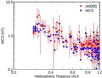
Fig. 3. Application of our procedure to data from Helios 2 (1976,
DOY 1 to 125). The blue markers represent deduced values for MCS for each day (the median of the hourly calculated MCS values), while the red markers represent the measured standard deviation of the magnetic field magnitude for each day (an average of the measured hourly values, with corresponding variation over each day shown by the error bars).
We compare these MCS values with the daily average of the hourly measured standard deviation of the ambient field magnitude (Fig. 3). Not surprisingly, the deduced values for MCS scale similarly to the variation in the magnetic field magnitude. However, inclusion of compressions in the mea-sured magnitude fluctuations often results in values higher than those our method produces for MCS. This is due to the fact that we only calculate MCS values for data periods with sufficiently low levels of compression.
6 Impact of heliospheric environment on calculation probability
We now apply our new method to obtain values for MCS and use them in the Leinweber et al. (2008) procedure to exam-ine the impact of our method on final offset calculation. In particular, we are interested in the probability of being able to deduce an offset, because it is still possible that a zero off-set cannot be calculated for a data period. For example, for data periods where the ambient field is consistently too com-pressional, the Leinweber et al. (2008) algorithm is unable to calculate the magnetic field offsets. Due to the strong depen-dence on Alfv´enicity, we examine the probability of being able to calculate an offset over a given data period at different solar wind speeds and heliospheric distances. As an example, if we are able to obtain an estimate of the offset in seven out of ten one-hour data periods in the dataset, that dataset has a calculation probability of 70 %.
We compare offset calculation probabilities for a range of data periods, solar wind speeds and heliocentric distances us-ing data from the Helios 2 spacecraft. Since fast flowus-ing solar wind is known to be more Alfv´enic than slow wind streams
Table 1. Heliospheric environment encountered by Helios 2 in
1976.
Heliospheric environment Day of year (DOY)
Fast solar wind 22–24, 32–33, 40–45, 49–52, 67–70,
75–78, 85, 94–98, 104–113
Slow solar wind 17–20, 26–31, 35–37, 46–47, 53–56,
72–73, 80–83, 88–91, 99–102, 123 125–126
Aphelion (0.90–1.00 AU) 1–47
Perihelion (0.29–0.40 AU) 95–120
(Mariani and Neubauer, 1990), and therefore less compres-sive, the algorithm should have a greater chance of calculat-ing an offset in fast wind streams. Days of fast and slow so-lar wind streams from 1976 are given in Table 1. As fast and slow solar wind streams collide, they merge and interact with one another, forming corotating interaction regions (CIRs) (Priest, 1995). Closer to the Sun, these CIRs are less promi-nent, but as they travel towards 1 AU the CIRs develop and become fully processed into a larger interaction region, re-sulting in a decreased Alfv´enicity (Kallenrode, 1998). There-fore, we anticipate higher calculation probabilities at peri-helion than apperi-helion. Days of apperi-helion and periperi-helion from 1976 are also given in Table 1.
We used our new method to calculate the MCS for each day of data during the heliospheric environments shown in Table 1. We then use these MCS values in the Leinweber et al. (2008) algorithm to calculate zero offsets for successive 10-min data periods over the total data length (a day of data). This process was then repeated for larger data periods, in-creasing by 10-min increments up to a data period of 2 h.
We also compared our new method with a fixed parameter approach that keeps MCS constant. For this fixed parame-ter comparison, at aphelion we chose MCS to have a value of 0.25 nT, which is consistent with the empirical values for MCS at these heliocentric distances used by Leinweber et al. (2008). At perihelion we deduced an appropriate fixed value of 1.5 nT for MCS, using an average of the calculated values for MCS shown in Fig. 3 between 0.29 and 0.40 AU.
Offset calculation probabilities for data periods between 10 min and 2 h are shown for fast and slow solar wind streams in Fig. 4. The probability of making an offset calculation is significantly higher for fast solar wind streams than slow so-lar wind streams. On average, a calculation probability of 70 % can be achieved by using a 40 min data period in fast solar wind and a 2 h data period in slow solar wind.
20m 40m 1h 1h 20m 1h 40m 2h 0
10 20 30 40 50 60 70 80 90 100
Data Period
Calculation Probability (%)
Fast Slow
Fig. 4. Offset calculation probabilities for fast and slow solar wind
from 1976, Helios 2 (specific dates in Table 1).
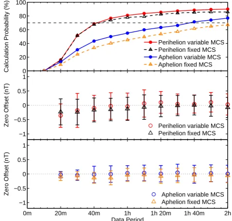
also find that our new method (using a variable MCS derived from the data itself) demonstrates an improvement in the cal-culation probability of 10 % at aphelion (beyond a time pe-riod of 40 min) and 4 % at perihelion (beyond a time pepe-riod of 1 h), when compared to the use of a fixed value for MCS.
The Helios 2 dataset for which we have calculated offsets has already been calibrated. Therefore we anticipate that the zero offsets we calculate should be close to zero. We find that there is no discernable difference in the calculated zero offsets using our automated method for determining MCS for offset correction compared to previous methods that used a fixed value for MCS. The values we find for the offsets are close to zero for both methods (Fig. 5b and c).
7 Conclusions
In order to improve the determination of magnetometer zero offsets, we have developed a new method that systematically deduces a key parameter related to the ambient compres-sional variance from the dataset without manual intervention. This parameter – namely the minimum compressional stan-dard deviation (MCS) – is used in the Leinweber et al. (2008) method in the selection criteria. These are checks that se-lect only data deemed sufficiently Alfv´enic and are critical to improving the accuracy of the offset calculated. We have compared our new method with previous work that uses a fixed parameter approach. Our new method demonstrates an improvement in the calculation probability of up to 10 % at aphelion and 5 % at perihelion. Equivalently, it reduces the typical data period required to achieve this calculation, e.g. a 70 % calculation probability by 16 % (20 min) at 1 AU.
Since the method favours incompressible magnetic field variations, and therefore strongly depends upon the Alfv´enicity of the solar wind, we have applied our method to different solar wind conditions observed by the Helios spacecraft. We have confirmed that we are more likely to
0 20 40 60 80 100
Calculation Probability (%
)
Perihelion variable MCS Perihelion fixed MCS Aphelion variable MCS Aphelion fixed MCS
−1 −0.5 0 0.5 1
Zero Offset (nT) Perihelion variable MCS
Perihelion fixed MCS
0m 20m 40m 1h 1h 20m 1h 40m 2h
−1 −0.5 0 0.5 1
Zero Offset (nT)
Data Period
Aphelion variable MCS Aphelion fixed MCS
Fig. 5. Top panel: offset calculation probabilities for aphelion and
perihelion 1976, Helios 2. Middle panel: average zero offsets cal-culated at perihelion. Bottom panel: average zero offsets calcal-culated at aphelion. The variable MCS points represent our new automated method and the fixed MCS points represent a comparison with pre-vious implementations of the Leinweber et al. (2008) algorithm.
be capable of calculating an offset during regions of fast so-lar wind compared to slow soso-lar wind, due to the increased Alfv´enicity and therefore reduced compressibility present in those faster streams. We also found that we are more likely to calculate offsets at perihelion than aphelion, due to fuller processing of CIRs towards aphelion, which results in a de-creasing of Alfv´enicity with heliospheric distance.
8 Further work
heliosphere – such as the Cassini magnetometer – due to the method’s sensitivity to heliocentric distance.
Acknowledgements. The authors would like to thank M. Delva for supplying Venus Express data for analysis, as well as providing an explanation of the calibration and correction procedure from raw data to offset measurement. We would also like to thank F. Neubauer for supplying additional high frequency Helios data. M. A. Pudney is grateful for the financial support from the STFC and Astrium Ltd.
Edited by: M. Rose
References
Acu˜na, M. H.: Space Based Magnetometers, Rev. Sci. Instrum., 73, 3717–3736, 2002.
Acu˜na, M., Curtis, D., Scheifele, J., Russell, C., Schroeder, P., Szabo, A., and Luhmann, J.: The STEREO/IMPACT Magnetic Field Experiment, Space Sci. Rev., 136, 203–226, 2008. Balogh, A.: Planetary Magnetic Field Measurements: Missions and
Instrumentation, Space Sci. Rev., 152, 23–97, 2010.
Belcher, J. W.: A Variation of the Davis-Smith Method for In-Flight Determination of Spacecraft Magnetic Fields, J. Geophys. Res., 78, 6480–6490, 1973.
Carr, C., Brown, P., Zhang, T. L., Gloag, J., Horbury, T., Lucek, E., Magnes, W., O’Brien, H., Oddy, T., Auster, U., Austin, P., Aydogar, O., Balogh, A., Baumjohann, W., Beek, T., Eichel-berger, H., Fornacon, K.-H., Georgescu, E., Glassmeier, K.-H., Ludlam, M., Nakamura, R., and Richter, I.: The Double Star magnetic field investigation: instrument design, performance and highlights of the first year’s observations, Ann. Geophys., 23, 2713–2732, doi:10.5194/angeo-23-2713-2005, 2005.
Davis, L. and Smith, E. J.: The in-flight determination of spacecraft magnetic field zeros, EOS Trans. AGU, 49, 257, 1968.
Hedgecock, P. C.: A correlation technique for magnetometer zero level determination, Space Sci. Instrum., 1, 83–90, 1975. Kallenrode, M.: Space Physics, Springer-Verlag, Berlin, 1998. Kepko, E. L., Khurana, K. K., Kivelson, M. G., Elphic, R. C., and
Russell, C. T.: Accurate determination of magnetic field gradi-ents from four point vector measuremgradi-ents: Use of natural con-straints on vector data obtained from a single spinning spacecraft, IEEE Trans. Magnet., 32, 377–385, 1996.
Kivelson, M. G.: Pulsations and Magnetohydrodynamic Waves, in: Introduction to Space Physics, edited by: Kivelson, M. G. and Russell, C. T., Cambridge University Press, 1995.
Leinweber, H. K., Russell, C. T., Torkar, K., Zhang, T. L., and An-gelopoulos, V.: An advanced approach to finding magnetometer zero levels in the interplanetary magnetic field, Meas. Sci. Tech-nol., 19, 055104, doi:10.1088/0957-0233/19/5/055104, 1998. Mariani, F. and Neubauer, F. M.: The Interplanetary Magnetic Field,
in: Physics of the Inner Heliosphere, edited by: Schwenn, I. R., Springer-Verlag, 1990.
Ness, N. F., Behannon, K. W., Lepping, R. P., and Schat-ten, K. H.: Use of Two Magnetometers for Magnetic Field Measurements on a Spacecraft, J. Geophys. Res., 76, 3564, doi:10.1029/JA076i016p03564, 1971.
Pope, S. A., Zhang, T. L., Balikhin, M. A., Delva, M., Hvizdos, L., Kudela, K., and Dimmock, A. P.: Exploring planetary magnetic environments using magnetically unclean spacecraft: a systems approach to VEX MAG data analysis, Ann. Geophys., 29, 639– 647, doi:10.5194/angeo-29-639-2011, 2011.