NUMERICAL AND ANALYTIC EXISTENCE OF PROPOSAL PROBLEM FORMULATION
Sameer Qasim
Department of Mathematics, College of Education, University of Al
ARTICLE INFO ABSTRACT
In this paper, we proved the convergence of the solution for the nonlinear fuzzy volterra integral classes equation over fuzzy interval with high computational and complexity t
analytical method, so we describable this solution by using Homotopy perturbation method, by using Banach fixed point theory for existence and uniqueness. That with explained numerical examples. Finally using the MAPLE program to so
Copyright©2016, Sameer QasimHasan and Alan Jalal
which permits unrestricted use, distribution, and reproduction in any medium, provided the original work is properly cited.
1. INTRODUCTION
In the last two decades with the rapid development of nonlinear science, there has appeared ever
and engineers in the analytical techniques for nonlinear problems. It is well known, that perturbation methods provide the mo versatile tools available in nonlinear analysis of engineering problems (Nguyen, 1978). The perturbation methods, like other nonlinear analytical techniques, have their own limitations. At first, almost all perturbation methods are based on the assum that a small parameter must exist in the equation. This so
perturbation techniques. As is well known, an overwhelming majority of nonlinear problems have no small parameters at all. Secondly, the determination of small parameters seems to be a special art requiring special techniques. An appropriate choice of small parameters leads to the ideal results, but an unsuitable choice may create serious problems. Furthermore, the approxima solutions solved by perturbation methods are valid, in most cases, only for the small values of the parameters. It is obvious that all these limitations come from the small parameter assumption. These facts have motivated to suggest alternate techniques, such variational iteration (He, 2000; Hillermeier, 2001), decomposition (Kaleva, 1987)
1997; Nayef, 1985) and iterative (Nguyen, 1978; Puri and Ralescu, 1983). In order to overcome these drawbacks, combining the standard homotopy and perturbation method, which is called the homotopy perturbation, modifies the homotopy method. problems in natural and engineering sciences are modeled by partial differential equations (PDEs). These equations arise in a number of scientific models such as the propagation of shallow water waves, long wave and chemical reaction
(Abbasbandy et al., 2007; Wu,1999). A substantial amount of work has been invested for solving such models. Several techniques including the method of characteristic, Riemann invariants, combination of waveform relaxation and multi
1990; Rajab et al., 2013; SushilaRathora et al
and Adomian’s decomposition (Rajab et al., 2013; SushilaRathora the solutions of such problems. Most of these techniques en
He (Klir et al., 1997; Park et al., 1995) developed the homotopy perturbation method for solving linear, nonlinear, initial and boundary value problems by merging two techniques, the standard homotopy and the perturbation technique. The homotopy
*Corresponding author: Alan jalalAbdulqader,
Department of Mathematics, College of Education, University of Al
ISSN: 0975-833X
Article History:
Received 15th May, 2016 Received in revised form 14th June, 2016
Accepted 10th July, 2016 Published online 31st July,2016
Citation: Sameer QasimHasan and Alan Jalal Abdulqader, International Journal of Current Research, 8, (07), 34829
Key words:
Fuzzy Number, Volterra nonlinear Integral equation, Operator of fuzzy number, fuzzy integral, fuzzy interval, Homotopy perturbation method.
RESEARCH ARTICLE
NUMERICAL AND ANALYTIC EXISTENCE OF PROPOSAL PROBLEM FORMULATION
OVER FUZZY INTERVAL
Sameer Qasim Hasan and *Alan Jalal Abdulqader
Department of Mathematics, College of Education, University of Al-Mustansiriyah, Baghdad Iraq
ABSTRACT
In this paper, we proved the convergence of the solution for the nonlinear fuzzy volterra integral classes equation over fuzzy interval with high computational and complexity t
analytical method, so we describable this solution by using Homotopy perturbation method, by using Banach fixed point theory for existence and uniqueness. That with explained numerical examples. Finally using the MAPLE program to solve our problem.
Jalal Abdulqader.This is an open access article distributed under the Creative Commons Att use, distribution, and reproduction in any medium, provided the original work is properly cited.
decades with the rapid development of nonlinear science, there has appeared
ever-and engineers in the analytical techniques for nonlinear problems. It is well known, that perturbation methods provide the mo ools available in nonlinear analysis of engineering problems (Nguyen, 1978). The perturbation methods, like other nonlinear analytical techniques, have their own limitations. At first, almost all perturbation methods are based on the assum
l parameter must exist in the equation. This so-called small parameter assumption greatly restricts applications of perturbation techniques. As is well known, an overwhelming majority of nonlinear problems have no small parameters at all. ermination of small parameters seems to be a special art requiring special techniques. An appropriate choice of small parameters leads to the ideal results, but an unsuitable choice may create serious problems. Furthermore, the approxima
by perturbation methods are valid, in most cases, only for the small values of the parameters. It is obvious that all these limitations come from the small parameter assumption. These facts have motivated to suggest alternate techniques, such
al iteration (He, 2000; Hillermeier, 2001), decomposition (Kaleva, 1987), expunction,
1997; Nayef, 1985) and iterative (Nguyen, 1978; Puri and Ralescu, 1983). In order to overcome these drawbacks, combining the topy and perturbation method, which is called the homotopy perturbation, modifies the homotopy method. problems in natural and engineering sciences are modeled by partial differential equations (PDEs). These equations arise in a
models such as the propagation of shallow water waves, long wave and chemical reaction
., 2007; Wu,1999). A substantial amount of work has been invested for solving such models. Several techniques characteristic, Riemann invariants, combination of waveform relaxation and multi
et al., 2012) periodic multi-grid wave form, variational iteration, homotopy perturbation ., 2013; SushilaRathora et al., 2012; Abbasbandy and Jafarian, 2006) have been used for the solutions of such problems. Most of these techniques en- counter the inbuilt deficiencies and involve huge computational work. ., 1995) developed the homotopy perturbation method for solving linear, nonlinear, initial and boundary value problems by merging two techniques, the standard homotopy and the perturbation technique. The homotopy
Department of Mathematics, College of Education, University of Al-Mustansiriyah, Baghdad Iraq.
International Journal of Current Research
Vol. 8, Issue, 07, pp.34829-34862, July, 2016
INTERNATIONAL
Abdulqader, 2016. “Numerical and analytic existence of proposal problem formulation over fuzzy interval, 34829-34862.
NUMERICAL AND ANALYTIC EXISTENCE OF PROPOSAL PROBLEM FORMULATION
Abdulqader
Mustansiriyah, Baghdad Iraq
In this paper, we proved the convergence of the solution for the nonlinear fuzzy volterra integral classes equation over fuzzy interval with high computational and complexity to find the solution in analytical method, so we describable this solution by using Homotopy perturbation method, by using Banach fixed point theory for existence and uniqueness. That with explained numerical examples.
open access article distributed under the Creative Commons Attribution License, use, distribution, and reproduction in any medium, provided the original work is properly cited.
- increasing interest of physicists and engineers in the analytical techniques for nonlinear problems. It is well known, that perturbation methods provide the most ools available in nonlinear analysis of engineering problems (Nguyen, 1978). The perturbation methods, like other nonlinear analytical techniques, have their own limitations. At first, almost all perturbation methods are based on the assumption called small parameter assumption greatly restricts applications of perturbation techniques. As is well known, an overwhelming majority of nonlinear problems have no small parameters at all. ermination of small parameters seems to be a special art requiring special techniques. An appropriate choice of small parameters leads to the ideal results, but an unsuitable choice may create serious problems. Furthermore, the approximate by perturbation methods are valid, in most cases, only for the small values of the parameters. It is obvious that all these limitations come from the small parameter assumption. These facts have motivated to suggest alternate techniques, such as , variation of parameters (Liao, 1997; Nayef, 1985) and iterative (Nguyen, 1978; Puri and Ralescu, 1983). In order to overcome these drawbacks, combining the
topy and perturbation method, which is called the homotopy perturbation, modifies the homotopy method. Many problems in natural and engineering sciences are modeled by partial differential equations (PDEs). These equations arise in a models such as the propagation of shallow water waves, long wave and chemical reaction-diffusion models ., 2007; Wu,1999). A substantial amount of work has been invested for solving such models. Several techniques characteristic, Riemann invariants, combination of waveform relaxation and multi-grid, (Wu and Ma, grid wave form, variational iteration, homotopy perturbation ., 2012; Abbasbandy and Jafarian, 2006) have been used for counter the inbuilt deficiencies and involve huge computational work. ., 1995) developed the homotopy perturbation method for solving linear, nonlinear, initial and boundary value problems by merging two techniques, the standard homotopy and the perturbation technique. The homotopy
INTERNATIONAL JOURNAL OF CURRENT RESEARCH
perturbation method was formulated by taking the full advantage of the standard homotopy and perturbation methods and has been applied to a wide class of functional equations. The basic motivation of the present paper is the implementation ofhis reliable technique for solving PDEs. In particular the proposed homotopy perturbation method (HPM) is tested on Helmholtz, Fisher’s, Boussinesq, singular fourth-order partial differential equations, systems of partial differential equations and higher-dimensional initial boundary value problems. The proposed iterative scheme finds the solution without any discretization, linearization or restrictive assumptions and is free from round off errors. The HPM gives the solution in the form of a convergent series with easily computable components. Unlike the method of separation of variables which requires both initial and boundary conditions, the HPM gives the solution by using the initial conditions only. The fact that the proposed HPM solves nonlinear problems without using Adomian’s polynomials can be considered as a clear advantage of this technique over the decomposition method.
2.Basic concepts
Basic definitions of fuzzy number are given in (1,2,10,15,17,20) as follows:
Definition 2.1.Fuzzy number.A fuzzy number is a map : → [ , ], which satisfying
(1)u is upper semi- continuous function, (2)u(x) = 0 outside some interval [a, d]
(3)There are real numbersb,c such a ≤ b ≤ c ≤ d
i)u(x)is a monotonic increasing function on [a, b]
ii)u(x) is a monotonic decreasing function on [c, d]
iii)u(x) = 1 for all x ∈ [b, c]
The set of all fuzzy numbers (as given by Definition 2.1) is denoted by E and is a convex cone. An alternative definition for parameter from of a fuzzy number is given by Kaleva (14).
Definition 2.2. A fuzzy number in parametric form is a pair ( , )of function ( ), ( ), ≤ ≤ , which satisfies the following requiremenst:
i) u(α)is a bounded left continuous non- decreasing function over (0, 1) ii) u(α)is a bounded left continuous non- increasing function over (0, 1) iii) u(α) ≤ u(α), 0 ≤ α ≤ 1
Definition 2.3. .For arbitrary fuzzy = ( ( ), ( )) , = ( ( ), ( )) , , ≤ ≤ and scalar , we define addition, subtraction, scalar product by and multiplication are respectively as following:
1 addition ∶ (u + v)(α)= (u(α)+v (α)), (u + v)(α) = (u(α)+v(α)),
2 subtraction ∶ (u v)(α)= (u(α)-v (α)), (u v)(α) = (u(α)-v(α)),
3 scalar product ∶
ku=
ku(α), ku(α) , k ≥ 0
ku(α), ku(α) , k < 0 ……….(1)
4- multiplication:
u v = uv(α) = max{u(α)v(α), u(α)v(α), u(α)v(α), u(α)v(α)}
uv(α) = min{u(α)v(α), u(α)v(α), u(α)v(α), u(α)v(α)} ………(2)
Defined 2.4.For arbitrary Fuzzy numbers u, v ∈ E
D(u, v) = max {sup ∈[ , ] u(α) v(α) , sup ∈[ , ] |u(α) v(α)|}, ………..(3)
In the distance between Theuandv, it is prove (E , D) is a complete metric space.
Definition 2.5. The integral of a fuzzy function was define in (14) by using the Riemann integral concept.
Let : [a, b]E . For Fuzzy function, for each partition p={t0, …, tn} of [a, b] and for arbitrary ξ ∈ [t , t ] , 1 ≤ i ≤ n, suppose
R =∑ f(ξ )(t t )
………...(4)
The define integral of f(t) over (a, b) is
∫ f(t)dt = lim → R , ………..(5)
If the fuzzy function f(t) is continuous in metric D,its definite the integral exists and also
(∫ f(t; α)dt ) =∫ f (t; α)dt, ( ∫ f(t; α)dt) = ∫ f (t; α)dt ………(6)
It should be noted that the fuzzy integral can be also defined using the Lebesgue – type approach. However, if f(t) is continuous, both approaches yield the same value .More details about the properties of the fuzzy integral
3.Proposal fuzzy nonlinear volterra integral classes equation
The fuzzy nonlinear integral equation with integral kernel which is discussed in this work is the fuzzy nonlinear Volterra integral equation (FNVIE2) as follows:
( ) = ( ) + ∫ , , , , ( ) ………(7)
where ≥ 0, ( )a fuzzy function of x : a ≤ x ≤ b, ( , ( , ( ) )) is analytic functions [ , ] , ( ) are nonlinear function on (a,b). For solving in parametric form of Eq. (7), consider ( ( , ), ( , )) and ( ( , ), ( , )) and, 0 ≤ ≤ 1 and t ,s∈(a,b) are parametric form of ( )and ( ), respectively. then, parametric form of Eq. (7) is as follows
( , ) = ( , ) + ∫ , , , , ( , ) ………...(8)
( , ) = ( , ) + , , , , ( , )
For each 0≤ ≤1 and a≤x≤b. We can see that Eq. (7) convert to a system of nonlinear Volterra integral equations in crisp case for each 0 ≤ ≤ 1 and a ≤ t ≤ b. Now, we explain analysis perturbation methods as approximating solution of this system of nonlinear integral equations in crisp case. then, we find approximate solutions for (x), a ≤ x ≤ b
We write the system (7) we obtain
( , ) = ( , ) + ∫ ( , , , , ( , ) + ∫ ( , , , , ( , ) ………(9)
( , ) = ( , ) + ( , , , , ( , ) + ( , , , , ( , )
where0 ≤ ≤ , ≤ ≤ , 0 ≤ ≤ 1
Now we will find the parameter for the Eq(7) , as follows
( , , , , ( , ) ) =
( , , , , ( , ) , ( , , , , ( , ) ≥ 0
( , , , , ( , ) , ( , , , , ( , ) < 0
, , ( , ) =
( , , ( , ) , , , ( , ) ≥ 0
( , , ( , ) , , , ( , ) < 0
, , ( , ) = ( , ( , ) , , , ( , ) ≥ 0
( , , ( , ) , , , ( , ) < 0
, , , , ( , ) =
( , , , , ( , ) , , , , , ( , ) ≥ 0
, , ( , ) = ( , ( , ) , , , ( , ) ≥ 0
( , , ( , ) , , , ( , ) < 0
, , ( , ) =
( , , ( , ) , , , ( , ) ≥ 0
( , , ( , ) , , , ( , ) < 0 … … … ….(10)
Than
( , ) = ( , ) + ( , , ( , , ( , ) + ( , , ( , ( , ) + ( , , ( , , ( , )
+ ( , , ( , , ( , )
( , ) = ( , ) + ∫ ( , , ( , ( , ) + ∫ ( , , ( , , ( , , ( , ) + ∫ ( , , ( , , ( , )
+∫ ( , , ( , , ( , ) ………(11)
where0 ≤ ≤ , ≤ ≤ , ≤ ≤ , ≤ ≤ , 0 ≤ ≤ 1
3.1 Homotopy Perturbation Method
Consider the fuzzy nonlinear volterra integral equation of the second kind
( ) = ( ) + , , , , ( )
Let
= ( , ) ( , ) ( , , ( , , ( , ) ( , , ( , ( , ) ( , , ( , , ( , )
( , , ( , , ( , ) = 0
( ) = ( , ) ( , ) ( , , ( , ( , ) ( , , ( , , ( , , ( , ) ( , , ( , , ( , )
∫ ( , , ( , , ( , ) = 0 ………..(12)
then we defined the homotopy
, , ( , )by
, 0 = , , 1 = ( )
( , 0) = ( ) , ( , 1) = ( )
where , ( ) are functional operators with solution say , which can be obtained easily. We choose a convex homotopy
, = (1 ) + = 0
( , ) = (1 ) ( ) + ( ) = 0 ……….……….(13)
and continuously trace an implicitly defined curve from a starting points , 0 , ( , 0) to a solution , 1 , ( , 1). The embedding parameter p monotonically increases from 0 to 1 as the trivial problem = 0 , ( ) = 0 continuously deformed to the original problem = 0,
( ) = 0. The parameter can be considered as an expanding parameter. In fact HPM uses the homotopy parameter p as an
expanding parameter to obtain
= + + + …
………..……..(14)
when → 1, (7) corresponding to (6) and gives an approximate as follows
= lim
→ + …
= lim → + ………(15)
The series (8) converges in most cases, and the rate of convergence depends on , ( )
Now we applied the HPM for solving system for fuzz volterra nonlinear integral equation
= ( , ) ( , )
( ) = ( , ) ( , )
, =
( , ) ( , ) ( , , ( , , ( , ) ( , , ( , ( , ) ( , , ( , , ( , )
( , , ( , , ( , ) = 0
( , ) =
( , ) ( , ) ( , , ( , ( , ) ( , , ( , , ( , , ( , ) ( , , ( , , ( , )
( , , ( , , ( , ) = 0
and equation the term with identical power of p , we obtain
: ( , ) ( , ) = 0 ( , ) = ( , )
: ( , ) ( , ) = 0 ( , ) = ( , )
: ( , ) ( , , ( , , ( , ) ( , , ( , ( , ) ( , , ( , , ( , )
( , , ( , , ( , ) = 0
( , ) = ( , , ( , , ( , ) + ( , , ( , ( , ) + ( , , ( , , ( , )
+ ( , , ( , , ( , )
: ( , ) ( , , ( , ( , ) ( , , ( , , ( , ) ( , , ( , , ( , )
( , , ( , , ( , ) = 0 ( , )
= ( , , ( , ( , ) + ( , , ( , , ( , ) + ( , , ( , , ( , )
+ ( , , ( , , ( , )
Now we will write the general formula for HPM to solve our system
( , ) = ∫ ( , , ( , , ( , ) + ∫ ( , , ( , ( , ) + ∫ ( , , ( , , ( , ) +
∫ ( , , ( , , ( , )
n=1,2,….
( , ) = ( , )
( , ) = ( , , ( , ( , ) + ( , , ( , , ( , ) + ( , , ( , , ( , )
+ ( , , ( , , ( , ) = 1,2, ….
Then if ( , ) is non negative and non positive we get
( , ) = ( , )
( , ) = ( , , ( , , ( , ) + ( , , ( , ( , ) + ( , , ( , , ( , )
+ ( , , ( , , ( , )
( , ) = ( , )
( , ) = ( , , ( , ( , ) + ( , , ( , , ( , ) + ( , , ( , , ( , )
+ ( , , ( , , ( , ) = 1,2, ….
3.1 Fuzzy integration of a crisp (real- valued) function over a fuzzy interval(Dubois, 1982a)
We shall consider a case for which Dubois and Prade(Dubois, 1982a) have proposed a fuzzy domain D of the real line R assumed to be delimited by two bounds in the following sense
( )
1
R 0 a0 bo
Fig. 1. Crisp valued function over a fuzzy interval
are fuzzy sets on R, whose membership function are and repectively , from R to (0,1).
∀ ∈ , ( )( ( )) evaluates to what extent x can be considered as a greatest lower bound ( respectively least
upper bound ) of D
are normalized fuzzy sets.
are convex fuzzy set
( , ), are assumed ordered in the sense that
= ≤ =
Definition 2 :Let ( ) be a real- valued mapping, and integerable on the interval
1 = , , f(u) over the domain de-limited is defined according to the extension principle by:
( , )( ) = , ∈ : ∫ ( ) min { ( ), ( )} ………..(12)
To develop an applicable numerical algorithm for computing fuzzy integration , it is very important to discuss the following useful remarks and propositions.
Remarks 1:
1-If one of he bounds is not fuzzy , we consider the integral of ( ) over [ , , and it’s membership function can be defined as (Dubois , 1980)
( , )( ) = : ∫ ( ) ( ) ………(13)
= : ( ) ( ) ( )
where F is an anti-derivative of f
2- If both bounds are fuzzy, then (2.1) can be rewritten as:
( , )( ) = ( ) ( )min{ ( ), ( )}
= ∈ min{ ( ), : ( ) ( ) ( )} ………..(14)
= ∈ min { ( ), ( , )( )}
The following are some of the useful properties
Proposition 1.(Dubois, 1982a)
Let ( ) be an anti-derivative function of f(x), i.e, ( ) = ∫ ( ) , for some ∈ ( the interval of integration) denoted is the image of the fuzzy set , defined by the extension principle ∀ ∈ ,
( )( ) = : ( ) ( ).
Moreover, denotes extended principle the following proposition holds:
∫ = ……….(15)
Proposition 2. (Dubois, 1982a)
Let be two real mapping integerable on interval I, ( : → , : → ) then :
∫ ( + ) ⊆ ∫ ⊕ ∫ ……….(16)
where⊆ denotes the usual fuzzy set inclusion , ⊕ denotes the extended additionproposition
3.(Dubois, 1982a)
If are both either positive or negative integerable real mapping
( : → , : → ) ( : → , : → ), then the equality holds , i.e
Proposition 4.(Dubois, 1982a)
Let be domains of R delimited by fuzzy bounds ( , ) and , respectively, then for any integerable mapping
∫ ⊆ ∫ ∫ ………(18)
where is delimited by ( , ), the equality holds if and only if is real number
Proof:
=
= ( ) ⊕ ( )
Not that ) ( = 0 if and only if is real number, otherwise
( ) = min { ( )( ), ( )( ), ( ̃)( ), ( )( )}}
≥ min ( )( ), ( )( ) = ( )
Since we add the constraint = , and we can drop ( ) which is normalized
Remarks 5.(Dubois, 1980)
, = ( ) ( ) is the value of the extended ( ) ( ) , =
Proof :
Let be the membership function of ,
( ) ( )
( ) = , : min { : ( ) ( ), : ( ) ( )}
= , : min { ( ), : ( ) ( )}
= , : ( ) ( ) min { ( ), ( )}
where
( ) ( ) = ( )
( , ) is the fuzzy value of the extended fuzzifying function :
= ( ) ( ), =
3.2. Numerical fuzzy integration of a crisp function over a fuzzy interval
We shall develop a computational algorithm for computing a numerical fuzzy integration of crisp function over a fuzzy interval. The basic principle of this technique for continuous fuzzy number. The continuous fuzzy number is discretized and then converted into discrete fuzzy number so that the numerical fuzzy integration over the discrete case can be easily implemented .
Mathematically, we can represent the fuzzy integration:
, = { ( ) | ( )
valued real function from R to R}
3.2.1 Fuzzy Integration for Discrete Fuzzy Numbers
general procedure for computing the fuzzy integration for discrete fuzzy numbers
A and B have been developed and as follows:
Let the universe set be , are discrete fuzzy numbers,
Then
= ( )/ , ∈
and
= ( )/ , ∈
Since are non empty fuzzy sets, then there are positive integer numbers, such that the support of the fuzzy sets can be given by :
= { , , … … . , } = { , , … … . , }
Let
= = ( )
Then define :
× = , ∈ , ∈ , = 1,2, … . . , = 1,2, … . . ,
Then let
× = ∫ × ( ) = ∫ ( ) ………..(19)
It should be noted that (19) is fuzzy set according to (2.1) where its membership function can be defined as:
× = , ∈ × min ( ), ( ) , = 1,2, … . . , , = 1,2, … . . ,
Let us define
, = ( )
If , = , , ≠ , ≠ . Then the supermum of this membership function of
, , , have been taken. Otherwise, no need for the supremum operation. Thus the fuzzy integration is:
, = {( × , × )| × = ( ) }
× Remark 2:
When , = ∫ ( ) = ∫ ( ) , fuzzy integrals are fuzzy sets with membership function
∫ ( ) ( ) = ∫ ( ) ( )
3.2.2. Fuzzy integration for continuous fuzzy numbers
= ∫ ( )\ , ∈
= ( )\ , ∈
Let us define the L.R type to represent the fuzzy numbers , where the membership function are defined as follows:
( ) =
, ≤
, ≥
……….(20)
( ) =
́
́ , ≤ ́
́
, ≥ ́
Then
= ( , , ) and
= ( ́ , ́ , )
Discretization of the above continuous fuzzy numbers can be done in two ways, and as follows:
3.2.2.1. Discretization of a abscissa ( )
Let ( ) be a continuous fuzzy number and ( ́ ) be the mean value of the fuzzy number ( ) with a membership value
( ) = 1, ( ( ́ ) = 1), ( ́ ) are left and right spreads of ( )( ( )), the membership function of the
continuous fuzzy number have unsharp boundaries. Furthermore , the reference function L (or R) for the fuzzy number is
decreasing on )0, +∞(, → ∞ , ( ) → 0
Step 1
Since the domain of the membership function which depending on LR-type , in general, it’s not bounded, so to find the lower limit and the upper limit for the reference function L and R respectively to find the boundaries of the membership function, then we have
If ≤ ( ≤ ́ ),
( ) = ( ) = ́
́
Since the membership function ( )( ( )) is continuous differentiable and decreasing function, therefore, there exists ∈ ( ∈ ), such that
| ( )| < and| ( )| <
, ( ) is called the lower bounds.
Similarly, if ≥ ( ≥ ́ ),
( ) = ( ) = ́
Since the membership function ( )( ( )) is continuous differentiable and decreasing function, therefore, there exists ∈ ( ∈ ), such that
, ( ) is called the upper bounds
Step 2:
A partition for the continuous fuzzy number centered at the mean v , m can be implemented and as follows:
Δ =| | (step length for left interval, where ≤ )
Δ =| | (step length for left interval, where ≥ )
Where
= lower limit of the membership function of of step 1 = upper limit of the membership function of of step 1 = mean value of the fuzzy number
, = l arge positive number
Similarly a partition for the continuous fuzzy number centered at the mean ́ divided into two partitions:
Δ =| ́ | (step length for left interval, where ≤ ́ )
Δ =| ́ | (step length for left interval, where ≥ ́ )
Where
= lower limit of the membership function of . = upper limit of the membership function of .
́= mean value of the fuzzy number
, = large positive number
Step 3:
Let = , then. For the left side discretized of membership function of the fuzzy number
, we have :
= , = 0,1,2, … . ,
with a membership function
( ) = ( )
For the right side discretized of membership function of the fuzzy number , we have :
= + , = 1,2, … . ,
with a membership function
( ) = ( )
Thus the approximate discrete fuzzy number for continuous fuzzy number can be rewritten as :
= { , ( ), … . . , ( , ( )), … . , ( , 1), ( , ( )), … . , ( ) , … . , , ( ) }
Similarly, let = ́ (mean value of the membership function of ), then. For the left side of membership function of the fuzzy number , we have :
with a membership function
( ) = (
́ )
For the right side discretized of membership function of the fuzzy number , we have :
= + , = 1,2, … . ,
with a membership function
( ) = ( )
the approximate discrete fuzzy number for continuous fuzzy number can be rewritten as :
= { , ( ), … . . , , ( ), … . , ( , 1), ( , ( )), … . ( , ( )), … . , , ( ) }
Step 4:
Take the support for the fuzzy number , then we have
= { , , … . , }
= { , , … . , ! }
= , = . ∶
× = {( , )| ∈ , ∈ , = 0,1, … . + , = 0,1,2, … , + }
Step 5:
For each ( , ) ∈ × ,calculate the integration
× = ( )
×
as has been discussed
× = ( , )∈ × min { , }
Step 6:
Check if , = , , ≠ , ≠ , then the supremum of this membership function of , , , have been take
Step 7:
Then the total fuzzy integration is :
, = {( , , ( , )| = 0,1, … . , , = 0,1, … . , }for some positive integers .
4. Solution of proposal fuzzy nonlinear integral classes equations
Our treatment of Crisp nonlinearvolterra integral equation classes mainly on illustrations of the known methods of finding exact, or numerical solution. In this work we present new techniques for solving crisp nonlinear volterra integral equations over the fuzzy interval. Re-writ equation (1)
( ) = ( ) + ∫ , , , , ( )
( , ) = ( , ) + ∫( )( ) ( , , , , ( , ) +∫( )( ) ( , , , , ( , )
( , ) = ( , ) + ( , , , , ( , )
( )
( )
+ ( , , , , ( , )
( )
( )
where (0) ≤ ≤ ( ) , ( ) ≤ ≤ ( ) , where (0) ≤ ≤ ( ) , ( ) ≤ ≤ ( )0 ≤ ≤ 1
than
( , ) = ( , ) + ( , , ( , , ( , ) + ( , , ( , ( , )
( )
( )
+
( )
( )
( , ,
( )
( )
( , , ( , )
+ ( , ,
( )
( )
( , , ( , )
( , ) = ( , ) + ∫( )( ) ( , , ( , ( , ) + ∫( )( ) ( , , ( , , ( , , ( , ) + ∫( )( ) ( , , ( , , ( , )
+∫( )( ) ( , , ( , , ( , )
………(21) where (0) ≤ ≤ ( ) , ( ) ≤ ≤ ( ), ( ) ≤ ≤ ( ), ( ) ≤ ≤ ( ),
(0) ≤ ≤ ( ), ( ) ≤ ≤ ( ), ( ) ≤ ≤ ( ), ( ) ≤ ≤ ( ), 0 ≤ ≤ 1
Remark1:
Let the = 0 ̃ = 1, = 0 = [ (0), (0)] = ( ( ), ( ))
̃ = [ ( ), ( )], = [ ( ), ( )], ̃ = [ ( ), ( )] (12)
Re-write the eq(12) with the fuzzy number formula
= 0 = [ (0), (0)] = 0 √1 , 0 + √1 = ( √1 , √1 )
= [ ( ), ( )] = √1 , + √1 = √1 , + √1
̃ = [ ( ), ( )] = √1 , + √1 = 0.5 √1 , 0.5 + √1
= [ ( ), ( )] = √1 , + √1 = 0.25 √1 , 0.25 + √1
̃ = [ ( ), ( )] = √1 , + √1 = 0.75 √1 , 0.75 + √1 …(21)
C=0.5 , d=0.25 , e=0.75
Substituting eq(21) in eq (1), we obtain
( , ) = ( , ) + ( , , ( , , ( , ) + ( , , ( , ( , )
( )
( )
+
( )
( )
( , ,
( )
( )
( , , ( , )
+ ( , ,
( )
( )
( , , ( , )
( , ) = ( , ) + ∫( )( ) ( , , ( , ( , ) + ∫( )( ) ( , , ( , , ( , , ( , ) + ∫( )( ) ( , , ( , , ( , )
We will use the all step in part 4 to find the solution of the system (2), . the numerical solution of the fuzzy function over the fuzzy interval using the LR-type representation of fuzzy interval. Some numerical examples are prepared to show the efficiency and accuracy of the methods
5. Numerical example
We will apply theHomotopy perturbation method to solve our problem and compared with the exact solution
Example 1
Consider the fuzzy nonlinear volterra integral equation
( ) = ( ) + , , , , ( )
Step 1
( , ) = ( , ) + ( , , , , ( , ) +
( )
( )
( , , , , ( , )
( )
( )
( , ) = ( , ) + ( , , , , ( , )
( )
( )
+ ( , , , , ( , )
( )
( )
where (0) ≤ ≤ ( ) , ( ) ≤ ≤ ( ) , where (0) ≤ ≤ ( ) , ( ) ≤ ≤ ( )0 ≤ ≤ 1
than
( , ) = ( , ) + ( , , ( , , ( , ) + ( , , ( , ( , )
( )
( )
+
( )
( )
( , ,
( )
( )
( , , ( , )
+ ( , ,
( )
( )
( , , ( , )
( , ) = ( , ) + ( , , ( , ( , )
( )
( )
+ ( , , ( , , ( , , ( , )
( )
( )
+ ( , ,
( )
( )
( , , ( , )
+∫( )( ) ( , , ( , , ( , )
where (0) ≤ ≤ ( ) , ( ) ≤ ≤ ( ), ( ) ≤ ≤ ( ), ( ) ≤ ≤ ( ), (0) ≤ ≤ ( ) , ( ) ≤ ≤ ( ),
( ) ≤ ≤ ( ), ( ) ≤ ≤ ( ), 0 ≤ ≤ 1
The exact solution
( , ) = , ( , ) = (2 )
The Kernal of our problem
( , , ( , , ( , ) = ^3( ( , ))^2
( , , ( , ( , ) = ^2( ( , ))^2
( , , ( , , ( , ) = ^3( ( , ))^2
( , , ( , , ( , ) = ^2( ( , ))^2
Remark1:
̃ = [ ( ), ( )], = [ ( ), ( )], ̃ = [ ( ), ( )] (12)
Re-write the eq(12) with the fuzzy number formula
= 0 = [ (0), (0)] = 0 √1 , 0 + √1 = [ √1 , √1 ]
= [ ( ), ( )] = √1 , + √1 = √1 , + √1
̃ = [ ( ), ( )] = √1 , + √1 = 0.5 √1 , 0.5 + √1
= [ ( ), ( )] = √1 , + √1 = 0.25 √1 , 0.25 + √1
̃ = [ ( ), ( )] = √1 , + √1 = 0.75 √1 , 0.75 + √1 ………(21)
C=0.5 , d=0.25 , e=0.75
Substituting eq(21) in eq (1), we obtain
( , ) = ( , ) + ( , , ( , , ( , ) + ( , , ( , ( , )
( )
( )
+
( )
( )
( , ,
( )
( )
( , , ( , )
+ ( , ,
( )
( )
( , , ( , )
( , ) = ( , ) + ∫( )( ) ( , , ( , ( , ) + ∫( )( ) ( , , ( , , ( , , ( , ) + ∫( )( ) ( , , ( , , ( , )
+∫( )( ) ( , , ( , , ( , )
We will use the all step in part 4 to find the solution of the system (2), . the numerical solution of the fuzzy function over the fuzzy interval using the LR-type representation of fuzzy interval. Some numerical examples are prepared to show the efficiency and accuracy of the methods
5. Numerical example
We will apply theHomotopy perturbation method to solve our problem and compared with the exact solution
Example 1
Consider the fuzzy nonlinear volterra integral equation
( ) = ( ) + ∫ , , , , ( )
Step 1
( , ) = ( , ) + ( , , , , ( , ) +
( )
( )
( , , , , ( , )
( )
( )
( , ) = ( , ) + ( , , , , ( , )
( )
( )
+ ( , , , , ( , )
( )
( )
where (0) ≤ ≤ ( ) , ( ) ≤ ≤ ( ) , where (0) ≤ ≤ ( ) , ( ) ≤ ≤ ( )0 ≤ ≤ 1
than
( , ) = ( , ) + ( , , ( , , ( , ) + ( , , ( , ( , )
( )
( )
+
( )
( )
( , ,
( )
( )
( , , ( , )
+ ( , ,
( )
( )
( , ) = ( , ) + ∫( )( ) ( , , ( , ( , ) + ∫( )( ) ( , , ( , , ( , , ( , ) + ∫( )( ) ( , , ( , , ( , )
+∫( )( ) ( , , ( , , ( , )
where
(0) ≤ ≤ ( ), ( ) ≤ ≤ ( ), ( ) ≤ ≤ ( ), ( ) ≤ ≤ ( ),
(0) ≤ ≤ ( ), ( ) ≤ ≤ ( ), ( ) ≤ ≤ ( ), ( ) ≤ ≤ ( ), 0 ≤ ≤ 1
The exact solution ( , ) = , ( , ) = (2 )
The Kernal of our problem
( , , ( , , ( , ) = ^3( ( , ))^2
( , , ( , ( , ) = ^2( ( , ))^2
( , , ( , , ( , ) = ^3( ( , ))^2
( , , ( , , ( , ) = ^2( ( , ))^2
Remark 1:
Let the = 0 ̃ = 1, = 0 = [ (0), (0)] = [ ( ), ( )]
̃ = [ ( ), ( )], = [ ( ), ( )], ̃ = [ ( ), ( )] (12)
Re-wirte the eq(12) with the fuzzy number formula
= 0 = [ (0), (0)] = 0 √1 , 0 + √1 = [ √1 , √1 ]
= [ ( ), ( )] = √1 , + √1 = √1 , + √1
̃ = [ ( ), ( )] = √1 , + √1 = 0.5 √1 , 0.5 + √1
= [ ( ), ( )] = √1 , + √1 = 0.25 √1 , 0.25 + √1
̃ = [ ( ), ( )] = √1 , + √1 = 0.75 √1 , 0.75 + √1
C=0.5 , d=0.25 , e=0.75
( , ) = ( , )
+ ( , , ( , , ( , ) + ( , , ( , ( , )
. √
. √
. √
√
+ ( , ,
. √
. √
( , , ( , ) + ( , ,
√
. √
( , , ( , )
( , ) = ( , ) + ∫
√. √( , ,
(
, ( , )
+ ∫
.. √√( , , ( , ,
( ,
, ( , )
+
∫
.. √√( , ,
( ,
, ( , )
+
∫
. √√( , ,
( ,
, ( , )
Now we will find the lift and right for ( )
( , )=
Step 2
( ) =
, ≤
, ≥
( ) =
́
́ , ≤ ́
́
, ≥ ́
Then
= ( , , )
and
= ( ́ , ́ , )
Discretization of the above continuous fuzzy numbers as follows:
Step 1 Let be continuous fuzzy number of the LR-type function and as follows, where
(0) = ( ( , )) = ( ) , ( ) = ( , ) = ( (2 ))^2
(0) = ( ) ( ) = ( (2 ))
Given the spread number = 2 , = 3 and m=0(mean value of the zero fuzzy number ). Then the membership function of he continuous zero fuzzy number can be represented as follows.
( ) =
L((0
2 ) )^2 ∈ [ 2/ , 0]
1 = 2/
( 30 ) ∈ [0,3/ ]
now we calculate , be a continuous fuzzy number of the LR-type function.
Given the spread number = 2 = 3 and ́=1(mean value of the one fuzzy number ) as follows:
( ) =
( 1
2 (2 ))^2, ∈ [ 1/(2 ),1]
1 = 1/(2 )
( 31 (2 )) ∈ [1,2 3 + 1]
Thus, the membership functions of the continuous zero fuzzy number ( ) and ( ) are bounded, where
= 2/ , = 3/
= 1/(2 ), = 3
2 + 1
step 3. A partition for the continuous zero fuzzy number can be as follows let = 0(mean value of zero fuzzy number ). For the left hand side,
=| |= 0.67
Also, for the right hand side, where ≤ , = 3
=| |= 1/
so, for the left side
= , = 0,1,2
with the membership function
( ) = ((
2 ) ) ^2
[image:18.595.160.432.402.447.2]where = 0 , = 2 = (( ) ) ^2. The following results of table 1 are obtained:
Table 1. Right speared of fuzzy number of lower bound
i ( )
0 0 0
1 -0.67 0.1122 ^4
2 -1.34 0.449 ^4
The right hand side
= , = 1,2,3,
with the membership function
( ) =
3 = (3)
where = 0 , = 3 = ( ) . The following results of table 2 are obtained:
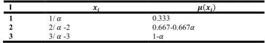
Table 2. left speared of fuzzy number of lower bound
I ( )
1 1/ 0.333
2 2/ -2 0.667-0.667
3 3/ -3 1-
Then, the approximate discrete fuzzy number for is
= {( , ( ))|i=0,1,2,3,4,5,6}
Similarly, a partition for the continuous one fuzzy number can be as follows = 1 (mean value of one fuzzy number ). For the left hand side, where
where ≥ , = 2,
=| |= 1/2 -1/2(2- )
Also, for the right hand side, where ≤ , = 3
=| |= 1/(2- )
so, for the left side
= , = 0,1,2
with the membership function
( ) = ((
where = 1 , = 2 = (( ) (2 )) ^2 . The following results of table 3 are obtained:
Table 3. Right speared of fuzzy number of upper bound
i ( )
0 1 O
1 1/2 1/4 2 1/4(1/2 + 1/4 2 )^2(2 )^2
2 2/4 2 1/4(1 2/4 2 )^2(2 )^2
The right hand side
= , = 1,2,3
with the membership function
( ) =
3 (2 ) = ( 3 )(2 )
where = 1 , = 3 = (2 ). The following results of table 4 are obtained:
Table 4. Left speared of fuzzy number of upper bound
i ( )
1 1-1/(2- ) 0.333
2 2-2/(2- ) 0.333(2- ) 0.667
3 3-3/(2- ) 0.667(2- ) 1
= {( , ( )| = 0,1, … . . ,6}
={(1,0),( 1/2-1/4-2α, 1/4(1/2+1/4-2α)^2(2-α)^2),( 2/4-2α, 1/4(1-2/4-2α)^2(2- α)^2),( 1+1/(2- ),0.333),( 2+2/(2- ),
0.333(2-) 0.667),( 3+3/(2- ), 0.667(2- ) 1)}
Step 2. Define approximately
× , ∈ , ∈ , = 0,1,2,3,4,5,6, , = 0,1,2,3,4,5,6, }
And then evaluate the integration on × , where
= ( )
= {( ( ), }
finally we use the HPM to find the solution
substitution or all = =
we have 36 values for lift sider and 36 for right side of the the equation with the Minimum membership function
( ) = {( ( )+I, , ( ( ( )+ , ))}
and finally we find the ( ) we have 36 values for lif and 36 for right of the equation with membership function
step 4. Check if , = , , 1 ≠ 2 , 2 ≠ 2, then
, = { , , , }
step 5. Finally, we have the total crisp nonlinear function over fuzzy integration
, = (0, 1)
= , , | = 0,1, … . , ∈ ; = 0,1, … . , ∈ }
The lower integral equation
, = 1.34 , 2
4 2 , 1.34 ,
1 2
1
4 2 , [ 1.34 , 1] ,
0.67 , 2
4 2 , 0.67 ,
1 2
1
4 2 , [ 0.67 , 1] ,
{ 0,2
4 2α ,
0,1 2
1
4 2α , [0,1]}
The upper integral equation and using the Remark 2
, = 1 1
2 ,
1
, 1 1
2 ,
2
2 , 1 1
2 , 3 3 , 2 2 2 , 1
, 2 2
2 ,
2
2 , 2 2
2 ,
3 3 ,
{ 3 3
2 ,
1
, 3 3
2 ,
2
2 , 3 3
2 ,
3 3 }
we will have 81 integral of the fuzzy intervals
Now we reduce the 9 integral for lower and 9 integral for upper
Now we will applied the HPM to solve our formula
( , ) = ( , ) = ( , ) = ( , ) = ( , ) = ( , , ( , , ( , ) + ( , , ( , ( , ) . √ . √ . √ √ + ( , , . √ . √ ( , , ( , ) + ( , , √ . √ ( , , ( , ) ( , ) = ∫( )( ) ( , , ( , ( , ) + ∫( )( ) ( , , ( , , ( , , ( , ) + ∫( )( ) ( , , ( , , ( , ) +∫( )( ) ( , , ( , , ( , )
And now we will find the value of the integration for the lower partition for interval by using HPM
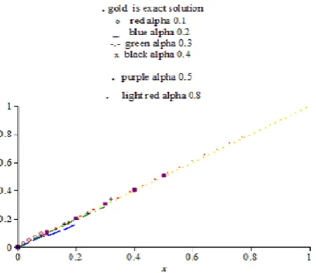
( , )in interval [ 1.34 , ]
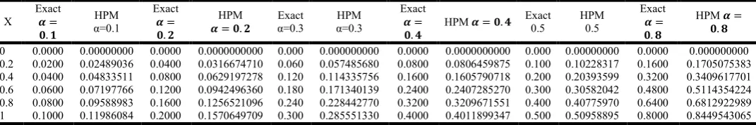
Table 1 . For lower bound interval(-1.34 ,2/4-2 ) for ( , )
X Exact = . HPM α=0.1 Exact = . HPM = . Exact α=0.3 HPM α=0.3 Exact = .
HPM = .
Exact = .
HPM = . Exact
= .
HPM = .
[image:21.595.47.553.199.492.2]0 0.0000 0.00000 0.0000 0.000000 0.000 0.000000000 0.0000 0.000000000 0.000 0.0000 0.0000 0.0000000000 0.2 0.0200 0.0249 0.0400 0.316674 0.060 0.057385673 0.0800 0.080645581 0.100 0.1015361920 0.1600 0.1634133051 0.4 0.0400 0.0483 0.0800 0.062919 0.120 0.114335743 0.1600 0.160571267 0.200 0.2024512711 0.3200 0.3267774894 0.6 0.0600 0.0719 0.1200 0.094249 0.180 0.171340120 0.2400 0.240727321 0.300 0.3035945575 0.4800 0.4901595691 0.8 0.0800 0.0958 0.1600 0.125652 0.240 0.228442746 0.3200 0.320965546 0.400 0.4047916926 0.6400 0.6529732694 1 0.1000 0.1198 0.2000 0.157064 0.300 0.285551307 0.4000 0.401187925 0.500 0.5058808041 0.8000 0.8100762465
Fig 1.Compared between the exact solution and HPM
( , , ( , , ( , ) + ( , , ( , ( , ) . √ . √ + . √ . ( , , . √ . √ ( , , ( , ) + ( , , . √ ( , , ( , )
Table 2. For lower bound interval [-1.34 ,1/2- 1/4-2 ] for ( , )
X Exact = . HPM α=0.1 Exact = . HPM = . Exact α=0.3 HPM α=0.3 Exact
= . HPM = .
Exact 0.5 HPM 0.5 Exact = . HPM = .
0 0.0000 0.0000 0.0000 0.000000 0.000 0.000000 0.0000 0.0000000 0.000 0.000 0.0000 0.00000 0.2 0.0200 0.024890 0.0400 0.03162591280 0.060 0.05727200217 0.0800 0.07995464738 0.100 0.100232548 0.1600 0.127734392 0.4 0.0400 0.048335 0.0800 0.06283785628 0.120 0.1139134510 0.1600 0.1592089707 0.200 0.199860092 0.3200 0.255440714 0.6 0.0600 0.071977 0.1200 0.09412721372 0.180 0.1707079694 0.2400 0.2386758324 0.300 0.299709918 0.4800 0.381572623 0.8 0.0800 0.095889 0.1600 0.1254889212 0.240 0.2275999625 0.3200 0.3182303024 0.400 0.399612396 0.6400 0.510548830 1 0.1000 0.119860 0.2000 0.1568609859 0.300 0.2844978439 0.4000 0.3977691990 0.500 0.499409237 0.8000 0.634664580
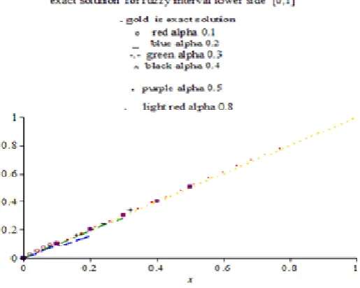
( , )in interval [ 1.34 , 1]
( , , ( , , ( , ) + ( , , ( , ( , ) . √ . √ + . √ . ( , , . √ . √ ( , , ( , ) + ( , , . √ ( , , ( , )
Fig. 2. Compared between the exact solution and HPM
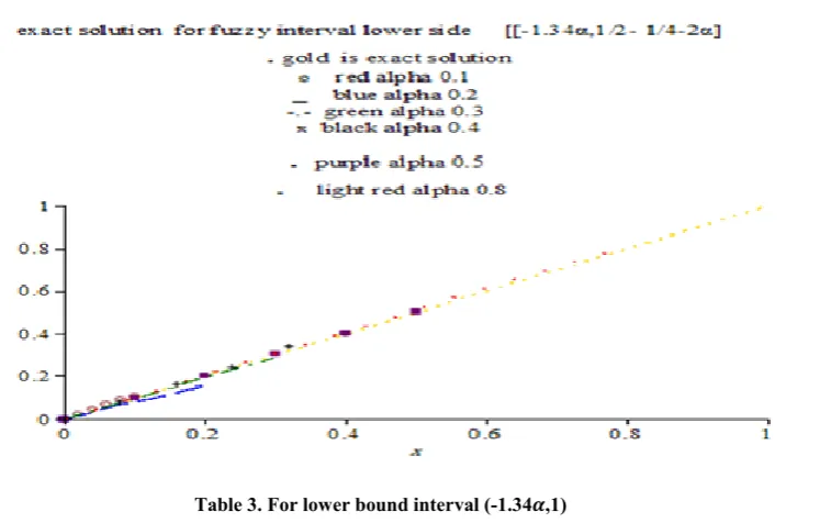
Table 3. For lower bound interval (-1.34 ,1)
x
Exact = .
HPM α=0.1
Exact = .
HPM = .
Exact α=0.3
HPM α=0.3
Exact = .
HPM = . Exact
0.5
HPM 0.5
Exact = .
HPM = .
0 0.0000 0.000000 0.0000 0.000000000 0.000 0.0000000000 0.0000 0.0000000000 0.000 0.0000000 0.0000 0.00000000 0.2 0.0200 0.024890 0.0400 0.032414231 0.060 0.0601750779 0.0800 0.0859703147 0.100 0.11014050 0.1600 0.15339961 0.4 0.0400 0.048336 0.0800 0.064390878 0.120 0.1196509785 0.1600 0.1711308488 0.200 0.21955355 0.3200 0.30675603 0.6 0.0600 0.071979 0.1200 0.096449444 0.180 0.1792967655 0.2400 0.2565372716 0.300 0.32923393 0.4800 0.46012815 0.8 0.0800 0.095892 0.1600 0.128584443 0.240 0.2390505471 0.3200 0.3426449136 0.400 0.43897758 0.6400 0.61300023 1 0.1000 0.119863 0.2000 0.160730379 0.300 0.2988108506 0.4000 0.4275345903 0.500 0.54859441 0.8000 0.76084497
Fig. 3. Compared between the exact solution and HPM
( , )in interval [ 0.67 ,
( )]
( , , ( , , ( , ) + ( , , ( , ( , )
. √
. √
+
. √
.
( , ,
. √
. √
( , , ( , )
+ ( ) ( , ,
. √
[image:22.595.36.542.449.751.2]Table 4. For lower bound interval (-0.67 ,2/4-2 ) X Exact = . HPM α=0.1 Exact = . HPM = . Exact α=0.3 HPM α=0.3 Exact = .
HPM = . Exact
0.5
HPM 0.5
Exact
= . HPM = .
0 0.0000 0.00000000 0.0000 0.0000000000 0.000 0.0000000000 0.0000 0.0000000000 0.000 0.00000000 0.0000 0.000000000
0.2 0.0200 0.02489036 0.0400 0.0316674671 0.060 0.0574855000 0.0800 0.0806441300 0.100 0.10227149 0.1600 0.1700003675
0.4 0.0400 0.04833511 0.0800 0.0629197203 0.120 0.1143354403 0.1600 0.1605753899 0.200 0.20912795 0.3200 0.3399477278
0.6 0.0600 0.71977659 0.1200 0.0942496248 0.180 0.1713396667 0.2400 0.2407230109 0.300 0.30578564 0.4800 0.5099143994
0.8 0.0800 0.09588984 0.1600 0.1256520946 0.240 0.2284421450 0.3200 0.3209598002 0.400 0.40771332 0.6400 0.6792677553
[image:23.595.28.545.175.507.2]1 0.1000 0.11986084 0.2000 0.1570649522 0.300 0.2855505512 0.4000 0.4011080742 0.500 0.50953101 0.8000 0.8424608540
Fig. 4. Compared between exact solution and HPM
( , )in interval [ 0.67 , ]
( , , ( , , ( , ) + ( , , ( , ( , ) . √ . √ + . √ . ( , , . √ . √ ( , , ( , ) + ( , , . √ ( , , ( , )
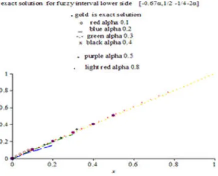
Table 5. For lower bound interval (-0.67 ,1/2 -1/4-2 )
X Exact = . HPM α=0.1 Exact = . HPM = . Exact α=0.3 HPM α=0.3 Exact = .
HPM = . Exact
0.5
HPM 0.5
Exact = .
HPM = .
0 0.0000 0.00000000 0.0000 0.0000000000 0.000 0.000000000 0.0000 0.000000000 0.000 0.00000000 0.0000 0.0000000000 0.2 0.0200 0.02489035 0.0400 0.3162615253 0.060 0.0572820565 0.0800 0.0800716923 0.100 0.10096785 0.1600 0.1596861526 0.4 0.0400 0.04833508 0.0800 0.0628383285 0.120 0.1139333220 0.1600 0.1594409309 0.200 0.20132161 0.3200 0.3193253834 0.6 0.0600 0.07197759 0.1200 0.0941279199 0.180 0.1707377154 0.2400 0.2390233567 0.300 0.30190100 0.4800 0.4789817086 0.8 0.0800 0.09588974 0.1600 0.1254898626 0.240 0.2276396199 0.3200 0.3186936556 0.400 0.40253383 0.6400 0.6380950806 1 0.1000 0.11986007 0.2000 0.1568621626 0.300 0.2845474149 0.4000 0.3983483347 0.500 0.50305945 0.8000 0.7917520887
[image:23.595.30.572.453.542.2] [image:23.595.195.414.577.753.2]∫ ( , , ( , , ( , ) + ∫.. √ ( , , ( , ( , ) √ + . √ . ∫ ( , , . √ . √ ( , , ( , ) + ∫. √ ( , , ( , , ( , )
Table 6. For lower bound interval (-0.67 ,1)
x Exact = . HPM α=0.1 Exact = . HPM = . Exact α=0.3 HPM α=0.3 Exact = .
HPM = . Exact
0.5 HPM 0.5 Exact = .
HPM = .
0 0.0000 0.00000000 0.0000 0.0000000000 0.000 00000000000 0.0000 0.0000000000 0.000 0.00000000 0.0000 0.0000000000
0.2 0.0200 0.02489056 0.0400 0.0324144705 0.060 0.0601851322 0.0800 0.0860873596 0.100 0.11087580 0.1600 0.1853513732
0.4 0.0400 0.04833603 0.0800 0.0643913516 0.120 0.1196708496 0.1600 0.1713628090 0.200 0.22101507 0.3200 0.3706406822
0.6 0.0600 0.07197926 0.1200 0.0964501500 0.180 0.1793265115 0.2400 0.2568847958 0.300 0.33142502 0.4800 0.5595260290
0.8 0.0800 0.09589200 0.1600 0.1285853843 0.240 0.2390920440 0.3200 0.3425082669 0.400 0.44189901 0.6400 0.7405464832
[image:24.595.31.552.247.693.2]1 0.1000 0.11986355 0.2000 0.1607315556 0.300 0.2988604215 0.4000 0.4281137260 0.500 0.55224462 0.8000 0.9179324782
Fig.6. Compared between exact solution and HPM
( , )in interval [0,2/(4 2 ) ]
( , , ( , , ( , ) + ( , , ( , ( , ) . √ . √ + . √ ( , , . √ . √ ( , , ( , ) + ( , , /( ) . √ ( , , ( , )
Table 7. For lower bound interval (0,2/4-2 )
X Exact = . HPM α=0.1 Exact = . HPM = . Exact α=0.3 HPM α=0.3 Exact = .
HPM = . Exact
0.5 HPM 0.5 Exact = .
HPM = .
[image:24.595.32.568.630.719.2]Fig. 7. Compared between exact and HPM
( , )in interval [0, ]
( , , ( , , ( , ) + ( , , ( , ( , )
. √
. √
+
. √
( , ,
. √
. √
( , , ( , )
+ ( , ,
. √
[image:25.595.30.572.420.507.2]( , , ( , )
Table 8. For lower bound interval (0,1/2-1/4-2 )
x
Exact = .
HPM α=0.1
Exact = .
HPM = .
Exact α=0.3
HPM α=0.3
Exact
= . HPM = .
Exact 0.5
HPM 0.5
Exact =
.
HPM = .
0 0.0000 0.00000000 0.0000 0.0000000000 0.000 0.0000000000 0.0000 0.0000000000 0.000 0.00000000 0.0000 0.0000000000 0.2 0.0200 0.02489035 0.0400 0.0316261563 0.060 0.0572822161 0.0800 0.0800735501 0.100 0.10097952 0.1600 0.1601933234 0.4 0.0400 0.04835081 0.0800 0.0628383360 0.120 0.1139336374 0.1600 0.1594446128 0.200 0.20134481 0.3200 0.3203394258 0.6 0.0600 0.07197759 0.1200 0.0941279312 0.180 0.1707381875 0.2400 0.2390288730 0.300 0.30193578 0.4800 0.4805027314 0.8 0.0800 0.09588974 0.1600 0.1254898775 0.240 0.2276402494 0.3200 0.3187010105 0.400 0.40258020 0.6400 0.6401196242 1 0.1000 0.11986072 0.2000 0.1568621813 0.300 0.2845482017 0.4000 0.3983575273 0.500 0.50311739 0.8000 0.7942455412
[image:25.595.193.419.557.752.2]( , )in interval [0,1]
( , , ( , , ( , ) + ( , , ( , ( , )
. √
. √
+
. √
( , ,
. √
. √
( , , ( , )
+ ( , ,
. √
[image:26.595.32.571.182.265.2]( , , ( , )
Table 9. For lower bound interval (0,1)
X
Exact
= .
HPM α=0.1
Exact
= .
HPM
= .
Exact α=0.3
HPM α=0.3
Exact
= .
HPM = . Exact
0.5
HPM 0.5
Exact =
. HPM = .
0 0.0000 0.0000000 0.0000 0.0000000000 0.000 0.0000000000 0.0000 0.000000000 0.000 0.00000000 0.0000 0.0000000000
0.2 0.0200 0.02490563 0.0400 0.0324144743 0.060 0.0601852918 0.0800 0.0860892175 0.100 0.11088748 0.1600 0.1858585440
0.4 0.0400 0.04833602 0.0800 0.0643913591 0.120 0.1196711650 0.1600 0.1713664909 0.200 0.22103827 0.3200 0.3716547246
0.6 0.0600 0.07197925 0.1200 0.0945016122 0.180 0.1793269837 0.2400 0.2568903121 0.300 0.33145979 0.4800 0.5574736254
0.8 0.0800 0.09589200 0.1600 0.1285853992 0.240 0.2390908334 0.3200 0.3425156217 0.400 0.44194539 0.6400 0.7425710269
[image:26.595.175.433.306.512.2]1 0.1000 0.11986354 0.2000 0.1067315743 0.300 0.2988612083 0.4000 0.4281229186 0.500 0.55230256 0.8000 0.9204259307
Fig.9. Compared between exact and HPM
Now we will find the upper side
( , ) = ∫( )( ) ( , , ( , ( , ) + ∫( )( ) ( , , ( , , ( , , ( , ) + ∫( )( ) ( , , ( , , ( , )
+∫( )( ) ( , , ( , , ( , )
And now we will find the value of the integration for the upper partition for interval by using HPM
( , ) =in interval 1 ,
∫ ./ √ ( , , ( , ( , ) + ∫ .. √ ( , , ( , , ( , , ( , )
√ + ∫ ( , ,
. √
. √ ( , , ( , )
+∫ ( , ,
. √ ( , , ( , )
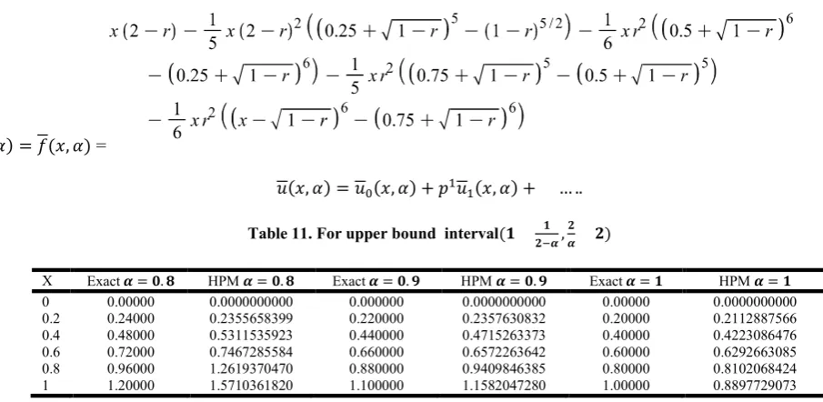
( , ) =
[image:27.595.46.481.245.489.2]( , ) = ( , ) + ( , ) + … ..
Table 10. For upper bound interval ( , )
x Exact = . HPM = . Exact = . HPM = . Exact = HPM =
0 0.00000 0.0000000000 0.000000 0.0000000000 0.00000 0.0000000000 0.2 0.24000 0.2411826921 0.220000 0.1832759126 0.20000 0.2370155469 0.4 0.48000 0.4823872965 0.440000 0.3665519962 0.40000 0.4737623581 0.6 0.72000 0.7235791148 0.660000 0.5947648550 0.60000 0.7063880020 0.8 0.96000 0.9644044580 0.880000 0.7810359563 0.80000 0.9131222690 1 1.20000 1.1991204420 1.100000 1.4260855860 1.00000 1.0184366070
Fig. 10.Compared between exact solution and HPM
( , ) =interval[1 , 2]
∫ . √ ( , , ( , ( , ) + ∫ .. √ ( , , ( , , ( , , ( , )
√ + ∫ ( , ,
. √
. √ ( , , ( , )
+∫ ( , ,
. √ ( , , ( , )
( , ) = ( , ) =
( , ) = ( , ) + ( , ) + … ..
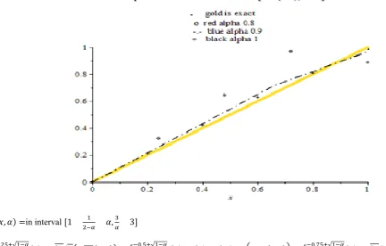
Table 11. For upper bound interval( , )
X Exact = . HPM = . Exact = . HPM = . Exact = HPM =
[image:27.595.62.515.540.761.2]Fig.11. Compared between exact and HPM
( , ) =in interval [1 , 3]
∫ ./ √ ( , , ( , ( , ) + ∫ .. √ ( , , ( , , ( , , ( , )
√ + ∫ ( , ,
. √
. √ ( , , ( , )
+∫ ( , ,
. √ ( , , ( , )
( , ) = ( , ) =
( , ) = ( , ) + ( , ) + … ..
Table 12. For upper bound interval ( , )
X Exact = . HPM = . Exact = . HPM = . Exact = HPM =
0 0.00000 0.0000000000 0.000000 0.0000000000 0.00000 0.0000000000 0.2 0.24000 0.3225929741 0.220000 0.2369682022 0.20000 0.2034439477 0.4 0.48000 0.6452078607 0.440000 0.4739365751 0.40000 0.4066196080 0.6 0.72000 0.9678099610 0.660000 0.7108417209 0.60000 0.6056734042 0.8 0.96000 1.2900455840 0.880000 0.9458051141 0.80000 0.7788359742 1 1.20000 1.6061718530 1.100000 1.1642303230 1.00000 0.8505786148
( , ) =in interval [2 , ]
∫ . √ ( , , ( , ( , ) + ∫ .. √ ( , , ( , , ( , , ( , )
√ + ∫ ( , ,
. √
. √ ( , , ( , )
+∫ . ( , ,
Fig.12. Compared between exact and HPM
( , ) = ( , ) =
Table 13. For upper bound interval( , )
X Exact = . HPM = . Exact = . HPM = . Exact = HPM =
[image:29.595.68.524.397.468.2]0 0.00000 0.0000000000 0.000000 0.0000000000 0.00000 0.0000000000 0.2 0.24000 0.2412112572 0.220000 0.1832768754 0.20000 0.1941272200 0.4 0.48000 0.4824450397 0.440000 0.3665539218 0.40000 0.4737623581 0.6 0.72000 0.7236657272 0.660000 0.5497677390 0.60000 0.7063882002 0.8 0.96000 0.9645197405 0.880000 0.7710397709 0.80000 0.9131223690 1 1.20000 1.1992624280 1.100000 0.8957734341 1.00000 1.0184366070
Fig. 13. Compared between exact and HPM
∫ . √ ( , , ( , ( , ) + ∫ .. √√ ( , , ( , , ( , , ( , ) + ∫ .. √√ ( , , ( , , ( , )
+∫ ( , ,
[image:29.595.139.467.515.703.2]( , ) = ( , ) =
Table 14. For upper bound interval( , )
6 Exact = . HPM = . Exact = . HPM = . Exact = HPM =
[image:30.595.44.486.260.512.2]0 0.00000 00.00000000 0.000000 0.0000000000 0.00000 0.0000000000 0.2 0.24000 0.3173362893 0.220000 0.2368530716 0.20000 0.2034439477 0.4 0.48000 0.6346944741 0.440000 0.4737663141 0.40000 0.4066191608 0.6 0.72000 0.9520398289 0.660000 0.7104963275 0.60000 0.6056734042 0.8 0.96000 1.269018609 0.880000 0.9453445555 0.80000 0.7788359742 1 1.20000 1.579880150 1.100000 1.1636544150 1.00000 0.8505786148
Fig.14. Compared between exact and HPM
( , ) =in interval [2 , 3]
∫ . √ ( , , ( , ( , ) + ∫ .. √√ ( , , ( , , ( , , ( , ) + ∫ .. √√ ( , , ( , , ( , )
+∫ ( , ,
. √ ( , , ( , )
[image:30.595.53.529.568.755.2]( , ) = ( , ) =
Table 15. For upper bound interval( , )
X Exact = . HPM = . Exact = . HPM = . Exact = HPM =
Fig.15. Compared between exact and HPM
( , ) =in interval [3 , ]
∫ . √ ( , , ( , ( , ) + ∫ . √ ( , , ( , , ( , , ( , )
. √ + ∫ ( , ,
. √
. √ ( , , ( , )
+∫ ( , ,
. √ ( , , ( , )
( , ) = ( , ) =
Table 16. For upper bound interval ( , )
X Exact = . HPM = . Exact = . HPM = . Exact = HPM =
0 0.00000 0.0000000000 0.000000 0.0000000000 0.00000 0.0000000000 0.2 0.24000 0.2415164175 0.220000 0.1833870386 0.20000 0.2370155464 0.4 0.48000 0.4805455060 0.440000 0.3665742478 0.40000 0.4894184899 0.6 0.72000 0.7245799693 0.660000 0.5947982028 0.60000 0.7298723978 0.8 0.96000 0.9657366339 0.880000 0.7831080036 0.80000 0.9444346324 1 1.20000 1.2007611690 1.100000 0.8958215553 1.00000 1.0575769370
( , ) =in interval [3 , 2]
∫ . √ ( , , ( , ( , ) + ∫ .. √ ( , , ( , , ( , , ( , )
√ + ∫ ( , ,
. √
. √ ( , , ( , )
+∫ ( , ,
. √ ( , , ( , )
Fig.16. Compared between exact and HPM
Table 17. For upper bound interval( , )
X Exact = . HPM = . Exact = . HPM = . Exact = HPM =
[image:32.595.47.499.459.713.2]0 0.00000 0.0000000000 0.000000 0.0000000000 0.00000 0.0000000000 0.2 0.24000 0.3158995633 0.220000 0.2357742090 0.20000 0.1829843206 0.4 0.48000 0.6318208463 0.440000 0.4715485889 0.40000 0.3659990600 0.6 0.72000 0.9477294128 0.660000 0.7077597195 0.60000 0.5442945229 0.8 0.96000 1.2632692250 0.880000 0.9410287187 0.80000 0.6969974660 1 1.20000 1.5726769090 1.100000 1.1582574080 1.00000 0.8897189433
Fig.17. Compared between exact and HPM
( , ) =in interval [3 , 3]
∫ . √ ( , , ( , ( , ) + ∫ .. √ ( , , ( , , ( , , ( , )
√ + ∫ ( , ,
. √
. √ ( , , ( , )
+∫ ( , ,
( , ) = ( , ) =
Table 18. For upper bound interval( , )
X Exact = . HPM = . Exact = . HPM = . Exact = HPM =
[image:33.595.141.462.263.478.2]0 0.00000 0.0000000000 0.000000 0.0000000000 0.00000 0.0000000000 0.2 0.24000 0.3229905027 0.220000 0.2375496642 0.20000 0.2112720136 0.4 0.48000 0.6460027211 0.440000 0.4750994989 0.40000 0.4222252925 0.6 0.72000 0.9690022249 0.660000 0.7175860846 0.60000 0.6291576019 0.8 0.96000 1.2916329750 0.880000 0.9481305388 0.80000 0.8101482378 1 1.20000 1.5081315960 1.100000 1.1671346830 1.00000 0.8897189433
Fig.18. Compared between exact and HPM
6- Conclusion
In this paper, the homotopy perturbation method has been successfully applied to find the solution of nonlinear fuzzy volterra integral classes equation over fuzzy interval. It is apparently seen that HPM is a very powerful and efficient technique in finding analytical solutions for complex classes of nonlinear problems. It is worth pointing out that this method presents a convergence for the solutions. The computations associated with the examples in this letter were performed using Maple 18.
REFERENCES
Abbasbandy S. and A. Jafarian, 2006.“Steepest descent method for solving fuzzy nonlinear equations,” Applied Mathematics and Computation, vol. 174, no. 1, pp. 669–675.
AbbasbandyS., E. Babolian, M. Alavi, 2007. Numerical method for solving linear Fredholm fuzzy integral equations of the second kind, Chaos Soliton and Fractals 31, 138146.
Chang, S. S. L.and Zadah, L. A. 1972.On fuzzy mapping and control. Trans. Systems, Man Cyberetics, SMC-2(1), 30-34. Chun. C. 2007. Integration using He’s homotopy perturbation method. Chaos, Solitons & Fractals, 34(4):1130–1134.
Cveticanin. L. 2006. Homotopy perturbation method for pure nonlinear differential equation. Chaos, Solitons & Fractals, 30:1221–1230.
Dubois D., H. Prade, 1978. Operation on fuzzy numbers, Int. J. System Science, 9, 613-626 http://dx.doi.org/10.1080/ 00207727808941724
Goestscel R. and W. Voxman, 1986. Elementary calculus. Fuzzy Sets and Systems, 18:31–34. Goetschel R. and Vaxman, 1986. Elementry fuzzy clculus, Fuzzy Sets and Systems, 18, 31-43
He. J. H. 1999. Homotopy perturbation technique. Comput. Methods Appl. Mech. Eng., 178(3-4):257–262.
He. J. H. 2000. A coupling method of homotopy technique and perturbation technique for nonlinear problems. Int. J. Nonlinear Mech., 35(3):37–43.
Hillermeier.C. 2001. Generalized homotopy approach to multiobjective optimization. Int. J. Optim. Theory Appl., 110(3):557– 583.
Kaleva. O. 1987. Fuzzy differential equations. Fuzzy Sets and Systems, 24:301–317.
KlirG. J., U. St. Clair, and B. Yuan, 1997.Fuzzy Set Theory: Foundations and Applications, Prentice-Hall, Eaglewood Cliffs, NJ, USA.
Liao. S. J. 1997. Boundary element method for general nonlinear differential operators. Eng. Anal. Boundary Element, 20(2):91– 99.
Liao. S. J. 1995. An approximate solution technique not depending on small parameters: a special example. Int. J. Non-Linear Mech., 30(3):371–380.
Nanda, S. 1989. On integration of fuzzy mappings. Fuzzy Sets and Systems, 32, 95-101. Nayef. A. H. 1985. Problem in perturbation. John Wiley, Stateplace, New York.
Nguyen. H. T. 1978. A note on the extension principle for fuzzy sets. J. Math. Anal. Appl., 64:369–380.
Ozis T. and A. Yildirim.2007. A note on He’s homotopy perturbation method for van der pol oscillator with very strong nonlinearity. Chaos, Solitons & Fractals, 34(3):989–991.
ParkJ.Y., Y.C. Kwan, J.V. Jeong, 1995. Existence of solutions of fuzzy integral equationsin Banach spaces, Fuzzy Sets and System, 72, 373-378
ParkJ.Y., Y.C.Kwan,J.V. Jeong, 1995. Existence of solution of fuzzy integral equations in Banach spaces, Fuzzy Sets and System, 72, 373- 378.
Puri M. L. and D. Ralescu. 1983. Differential for fuzzy function. J. Math. Anal. Appl., 91:552–558. Puri M. L. and D. Ralescu. 1986. Fuzzy random variables. J. Math. Anal. Appl., 114:409–422.
RajabN. A., A. M. Ahmad, O. M. Alfaour, 2013. Reduction Formula for Linear Fuzzy Equation, Applied Science Department, University of Technology Baghdad – Iraq.
SiddiquiA. M., R. Mahmood, and Q. K. Ghori. 2008. Homotopy perturbation method for thin film flow of a third grade fluid down an inclined plane. Chos, Solitons & Fractals, 35(1):140–147.
Sushila Rathora, Devendra Kumar, Jagdev Singh, SumitGapta, Homotopy, 2012. Analysis Method for Non Linear Equation, Department of Mathematics, Jagon Meth, University Village – Rampun Tehsil Chaksu, Jaipur – 303901, Ragashtan – India. Wu C. and M. Ma.1990. On the integrals, series and integral equations of fuzzy set-valued functions. J. Harbin Inst. Technol.,
21:11–19.
Wu, H.C. 1999. The improper fuzzy Riemann integral and its numerical integration, Information Science, 111, 109-137.