Toward a PV based algorithm for the dynamical core of hydrostatic global models

Toward a PV-Based Algorithm for the Dynamical Core of

Hydrostatic Global Models

ALIR. MOHEBALHOJEH

Institute of Geophysics, University of Tehran, Tehran, Iran

MOHAMMADJOGHATAEI

Institute of Geophysics, University of Tehran, Tehran, and Department of Physics, Yazd University, Yazd, Iran

DAVIDG. DRITSCHEL

School of Mathematics and Statistics, University of St. Andrews, St. Andrews, United Kingdom

(Manuscript received 25 October 2015, in final form 16 February 2016)

ABSTRACT

The diabatic contour-advective semi-Lagrangian (DCASL) algorithms previously constructed for the shallow-water and multilayer Boussinesq primitive equations are extended to multilayer non-Boussinesq equations on the sphere using a hybrid terrain-following–isentropic (s–u) vertical coordinate. It is shown that the DCASL algorithms face challenges beyond more conventional algorithms in that various types of damping, filtering, and regularization are required for computational stability, and the nonlinearity of the hydrostatic equation in thes–ucoordinate causes convergence problems with setting up a semi-implicit time-stepping scheme to reduce computational cost. The prognostic variables are an approximation to the Rossby– Ertel potential vorticityQ, a scaled pressure thickness, the horizontal divergence, and the surface potential temperature. Results from the DCASL algorithm in two formulations of thes–ucoordinate, differing only in the rate at which the vertical coordinate tends touwith increasing height, are assessed using the baroclinic instability test case introduced by Jablonowski and Williamson in 2006. The assessment is based on com-parisons with available reference solutions as well as results from two other algorithms derived from the DCASL algorithm: one with a semi-Lagrangian solution forQand another with an Eulerian grid-based solution procedure with relative vorticity replacingQas the prognostic variable. It is shown that at in-termediate resolutions, results comparable to the reference solutions can be obtained.

1. Introduction

Construction of potential vorticity (PV)-based models has been the subject of various individual studies (Charney 1962;Bates et al. 1995;Li et al. 2000;Mohebalhojeh and Dritschel 2004). The main objective of such models is to improve the representation of PV and thus simulate vortical flows with higher accuracy than conventional

models. This is important, as vortical flows comprise a significant part of the dynamical phenomena from large scales to mesoscales, including cyclones and fronts (Hoskins et al. 1985;Hsu and Arakawa 1990;Arakawa et al. 1992).

With regard to the material conservation of PV in the absence of diabatic and dissipative processes, it has been noted previously that one may gain higher numerical accuracy and/or computational efficiency by incorpo-rating Lagrangian information within the procedure for time integrating PV. Among these, the contour-advective semi-Lagrangian (CASL) algorithm and its extension to include sources and sinks of PV, that is, the diabatic contour-advective semi-Lagrangian (DCASL) algorithm, have repeatedly shown their potential to increase the ac-curacy of representing the vortical flow as well as the Corresponding author address: Ali R. Mohebalhojeh, Institute of

Geophysics, University of Tehran, P.O. Box 14155–6466, Tehran 1435944411, Iran.

E-mail: [email protected]

Denotes Open Access content.

DOI: 10.1175/MWR-D-15-0379.1

representation of imbalance (Mohebalhojeh and Dritschel 2007,2009). Within such numerical algorithms, PV as a defining variable for the vortical flow is given the highest priority in terms of accuracy. The sharp PV gradients generated horizontally by nonlinear advection are cap-tured by CASL/DCASL well beyond the capabilities of conventional grid-based algorithms. This brings with it the necessity of handling small horizontal scales associ-ated with sharp PV gradients. To address this issue, for thef-plane shallow-water (SW) equationsMohebalhojeh and Dritschel (2000)introduced the idea of implicitly using balance relations (Hoskins et al. 1985; McIntyre and Norton 2000;Mohebalhojeh and Dritschel 2001) through new sets of prognostic variables to represent unbalanced flow, alongside PV as the variable for vortical flow. Since then, the idea has been successfully applied to the SW equations on the sphere (Mohebalhojeh and Dritschel 2007, 2009; MirRokni et al. 2011) and the equatorial bplane (Mohebalhojeh and Theiss 2011), the many-layer isopycnal f-plane model (Mohebalhojeh and Dritschel 2004), and the two-layer isentropic Boussinesq model on the sphere (Mirzaei et al. 2012). It was also argued in

Mohebalhojeh and Dritschel (2004) that in problems involving a large number of layers, the issue with sharp PV gradients is compounded since large shearing motion in the vertical direction tends to generate substantial small-vertical-scale activity in both balanced and un-balanced flows. Associated with this, fictitious generation of imbalance in small vertical scales is inevitable. As a device to gain control on the small vertical scales of im-balance,Mohebalhojeh and Dritschel (2004)introduced and applied the idea of vertical-mode-dependent di-vergence damping.

Considering both accuracy and computational effi-ciency, the latter studies have pointed to the pair of horizontal velocity divergence dand horizontal accel-eration divergencegvariables, referred to as (d,g), as a viable candidate for extensions to more complicated sets of equations in our systematic exploration of models. While the non-Boussinesq extension of the two-layer isentropic model ofMirzaei et al. (2012)poses no great difficulty, the use of (d,g) variables has turned out to be hugely more difficult when a generalized vertical co-ordinate j is used, as discussed below. The problem becomes acute as the number of layers increases to that commonly used in the dynamical core of hydrostatic global models, which is the main objective of our current work. To raise the issues involved, and for continuity with our previous work, aspects of the DCASL algo-rithm based on the (d,g) variables are presented. However, the focus is on the DCASL algorithm that replaces horizontal acceleration divergence g with pressure thickness›p/›j.

The potential temperatureu is the other materially conserved quantity in the absence of diabatic and dis-sipative processes, and it has attracted considerable at-tention in numerical modeling (Bleck et al. 2010). The layer-wise two-dimensional structure of atmospheric– oceanic flows can be naturally modeled usinguas the vertical coordinate. Even though the resulting isentropic models have the potential to give a better representation of baroclinic waves, cyclones, and fronts, the issue of the intersection of isentropic surfaces within the ‘‘Under-world,’’ in the terminology ofHoskins (1991), with bottom topography has proved particularly difficult to resolve. The massless layer approach devised originally byBleck (1984)

gives poor results near the surface (Konor and Arakawa 1997), making it unsuitable for practical purposes when an accurate representation of surface features is needed. Another approach to the problem is to combine one of the terrain-following s coordinates with the isentropic coordinate in such a way that the resulting hybrid s–ucoordinate shares the benefits ofsat lower levels near the ground anduhigher up.

Using a hybrids–ucoordinate,Konor and Arakawa (1997)apply both mass continuity and thermodynamic energy equations at half-integer levels and find inter-polation relations for the pressurepandufields at full (integer) levels from the neighboring half-integer levels, in such a way as to satisfy energy conservation. The vertical mass flux is then obtained by the requirement that the time-discrete solutions forpandu remain on their defined coordinate surfaces. With the explicit re-lation defined for the hybrid coordinate, mathematically only the solution to one of the two fields ofpanduis required. The other field can be diagnosed from the definition of the coordinate surface. Here the pressure thickness of the layers is taken as the prognostic variable, and the u field is diagnosed. The vertical differencing remains the same as inKonor and Arakawa (1997), and the vertical mass flux is determined through a diagnostic relation obtained by setting the time derivative of the hybrid vertical coordinate to zero.

Williamson (2006a). This is a stringent test case for PV-based algorithms, as the instability is concentrated at low levels where the vertical coordinate substantially deviates fromuand thus there is a large source coming from vertical advection. Nevertheless, it is shown that the DCASL algorithms at intermediate resolutions can give solutions comparable to the reference solutions in

Jablonowski and Williamson (2006a,b)as well as those for a host of other dynamical cores inLauritzen et al. (2010).Section 5gives our concluding remarks.

2. Formulation

We consider the spherical hydrostatic primitive equations under the shallow-atmosphere approximation (Kasahara 1974; Thuburn 2011) and with continuous stratification represented by a generalized vertical co-ordinate. In their adiabatic, frictionless form, the gov-erning equations read

DV

Dt 1f​^k3V5 2=M1 P=u, (2.1a)

›M

›j 5 P ›u

›j, (2.1b)

› ›t

›p

›j

1=

V›p

›j

1 ›

›j

_ j›p

›j

50, and (2.1c)

Du

Dt50 , (2.1d)

whereD/Dt[›/›t1V=1j›_ /›jis the material deriv-ative,Vis the horizontal velocity vector,f52VEsinf

is the Coriolis parameter withVEbeing the rotation rate

of the sphere andfbeing the latitude,k is the unit vector^ in the local vertical direction, M is the Montgomery potential,uis potential temperature,jis the generalized vertical coordinate withj_its associated vertical velocity, andP [cp(p/p0)k is the Exner function withk5R/cp.

Here,R andcp are the gas constant and specific heat

capacity at constant pressure for dry air. In(2.1) and hereafter, the=and=are, respectively, the horizontal gradient and divergence operators.

To define vertical modes and construct a semi-implicit time integration scheme, a resting basic state in hydro-static balance is defined whose variables are denoted by an overbar. The basic state is considered a function of the vertical coordinate only. Any variable can be decomposed into a contribution from the basic state and a perturbation; thus, for example,P 5 P 1 P0. In this way, the right-hand side of(2.1a)can be written as

2=P01 P0=u0, where P5M2 Pu, P05M02 Pu05

F0_{1 P}0_{u, withFbeing the geopotential. For reference,}

hereafterP0is called ‘‘modified pressure.’’ By defining a nondimensional perturbation depth or pressure thickness

variableh~through›p/›j5›p/›j(11h~), it is convenient to rewrite the mass continuity equation [(2.1c)] as

›h~

›t1=[V(11h~)]1

1 ›p

›j › ›j

_ j›p

›j

50 , (2.2)

to bring it into the same form used in the SW equations with an apparent source due to vertical mass flux divergence.

a. Vertical modes

FollowingTemperton (1984), the primitive equations linearized around a basic state at rest are recast in the form of the SW equations by finding a matrixCsuch that

›P0

›t 5 2Cd, (2.3)

whereP0is the column vector (P0₁,P₂0,. . .,P0_L)T withL

being the number of layers and the T denoting trans-pose. The column vectordof the horizontal divergence is defined similarly. While it is possible to obtain the discrete analog of(2.3)for the vertical differencing of

Konor and Arakawa (1997)given later insection 3c, we will follow a different route. The reason is that, by fol-lowingKonor and Arakawa (1997), the resulting matrix

C is nonsymmetric, and the vertical modes are non-orthogonal for arbitrary stratification of the basic state. Here, instead, we first find the continuous equation for the time tendency ofP0and then vertically discretize it in such a way as to ensureCis symmetric. For our purpose the vertical modes serve as a set of basis functions with desirable properties that help control small-scale verti-cal structures, help solve the elliptic equation arising when the (Q,d,g) representation is used, and facilitate a semi-implicit solution procedure.

To obtain the matrix formulation, we write the verti-cal derivative of the tendency ofP0as

› ›j

›P0

›t 5H. (2.4)

To find the right-hand side functionH, the hydrostatic equation [(2.1b)] is first written as

›P0

›j 5 P

0›u

›j2u

0›P

›j, (2.5)

and then time differentiated, which after some manip-ulation leads to

H5

kP

p

›u ›j

›p0

›t 2

›P ›j

›u0 ›t 1 P

0›

›j ›u0

›t. (2.6)

v5›p

0

›t 1V=p1j_

›p

›j, (2.7)

v5V=p1v^, and (2.8)

^

v5 2

ðj

j_top =

V›p

›j

dj, (2.9)

withjtopthe value ofjat the top of the model andv^as an

auxiliary variable, are used to rewrite the thermody-namic energy equation [(2.1d)] as

›u0

›t5 2V=u 0₂ ›u ›j ›p ›j ^ v2›p

0

›t

. (2.10)

Noting thatkP/p5›P/›p, we can then writeHas

H5›P 0

›p

›u ›j

›p0

›t 1

›P ›p

›u ›jv^1

›P ›j V=u

0_{1 P}0›

›j ›u0

›t.

(2.11)

Then, we multiply(2.4)by›j/›pand vertically integrate the result from the middle of the layer with pressurepto the surface with pressureps

›P0

›t 5

›P0_s

›t 2

ðp_s

p

H›j

›pdp. (2.12)

In P0_s and similar terms, the subscript s refers to the surface value of the quantity. The surface term on the right-hand side of(2.12)can be written as

›P0_s

›t 5 2P 0

V_s=u01RTs

p_s

›p_s

›t

5 2P0_V

s=u

0₂RTs

p_s

ðj_s

j_top =

V›p

›j

dj. (2.13)

DefiningGandHas the column vectors of, respectively, ›P0/›tandH›j/›p,(2.12)can be written in matrix form as

G5G_s2AH, (2.14)

where A5 2 6 6 6 6 6 6 6 6 6 6 6 6 4

(Dp)₁

2 (Dp)2 . . . (Dp)L

0 (Dp)2

2 . . . (Dp)L

0 0 ⋱ ...

0 0 . . . (Dp)L

2 3 7 7 7 7 7 7 7 7 7 7 7 7 5

5Udiag[(Dp)] and

(2.15)

G_s5G_s(1, 1,. . ., 1)T, (2.16)

in which diag[(Dp)] is the diagonal matrix whose elements are (Dp)₁, (Dp)₂,. . ., (Dp)_L with (Dp)_l5p_l11/22p_l21/2. The vectorsG_sandHcan be decomposed into linear and nonlinear parts, that isG_s5G_s,l1G_s,nlandH5H_l1H_nl, where

G_s,l5 2RTs

p_s Ediag[(Dp)]d and (2.17)

H_l5 2diag

DP Dp

›u

›pLdiag[(Dp)]d, (2.18)

with (DP)_l5 Pl11/22 Pl21/2. Here, Gs,l and Hl result

from manipulating the second terms on the right-hand sides of, respectively,(2.13)and(2.11). The upper and lower triangular matricesUandLare defined by

U5 0 B B B B B B B B B B B @ 1

2 1 . . . 1

0 1

2 . . . 1

0 0 ⋱ ...

0 0 . . . 1 2 1 C C C C C C C C C C C A and (2.19) L5 0 B B B B B B B B B B B @ 1

2 0 . . . 0

1 1

2 . . . 0 ... 1 ⋱ 0

1 1 . . . 1 2 1 C C C C C C C C C C C A , (2.20)

and the matrixEhas 1 for every element. Using(2.14), one can obtain the matrixCas

C5

(

RT_s

p_s E2Udiag

›P

›p(Dp)

›u ›p

L

)

diag[(Dp)] ,

(2.21) which is the generalization of the matrix (2.34) of

matrix formulation, the vertical discretization only comes into play in approximating the integrals in-volved in(2.12)and in the linearized form of(2.9), for which the midpoint rule is used together with the ap-proximationp_l5(p_l11/21p_l21/2)/2 to reach a symmetric matrix. It should be stressed that there is no conflict in making the above choice for the full-level basic-state pressurepand using the pressurepcoming from the re-lation(3.16b)introduced later for the actual vertical dif-ferencing of the model.

Any matrix of the form UDL with D as a diagonal matrix is symmetric. This property and symmetry of

E make C symmetric. The eigenvectors and eigen-values of the matrixCare used to define the vertical modes and vertical-mode decomposition. To this end, the decomposition C5WLW21 is employed, where W and L are, respectively, the matrix of ei-genvectors and the diagonal matrix of eigenvalues of

C. For a general column vectorXin physical space, its projection onto the vertical mode space is defined byX5W21X.

Let us define a column vectorh, not to be confused with the perturbation depth variableh~, by h5C21P0. Now note that h5W21(WL21W21)P0 and thus

hm5l2m1P0mfor the vertical modemwith the eigenvalue

lm. The momentum equation [(2.1a)] linearized around

the resting basic state together with(2.3)then become equivalent to the linearized SW equations upon pro-jection to vertical modes:

›V0

›t 1f^k3

V05 2L=h and (2.22a) ›h

›t5 2d. (2.22b)

It is now evident from(2.22)that we can identify the eigenvalues with the squared gravity wave speeds in the shortwave limit, namely,lm5c2m.

b. Vertical velocity

To evaluate the time tendency of modified pressure from(2.4)and(2.6), the generalized vertical velocityj_is required. Taking the local time derivative ofj5F(s,u), withsdefined according to

s5 ps2p

p_s2p_top, (2.23)

the following diagnostic equation can be obtained

_

j5 2 1

p_s2p_top

^

v2(12s)›ps

›t

›F

›s

2›F

›uV=u. (2.24)

In(2.23),psis the surface pressure,ptopis the pressure at

the top of the model, and ›ps/›t5v^(js) is computed

diagnostically from(2.9). For conservation of total en-ergy, in deriving(2.24)ptophas taken to be constant (see

Konor and Arakawa 1997). One may also take the total derivative ofj5F(s,u) and come up with the alterna-tive form j_5(›F/›s)s_ for vertical velocity. Using the identity=j50, which holds onjsurfaces, it is not dif-ficult to show that the latter form and(2.24)are equiv-alent in the continuous limit. The time tendency of modified pressure also requires the time tendency of pressure, which is evaluated using

›p0

›t 5v^2j_

›p

›j. (2.25)

One potential problem with the use of the diagnostic estimate forj_is that an independent estimate for›p/›j is then required at half-integer levels wherej_resides. Alternatively, the same procedure leading to(2.24)can be modified to give us directly a diagnostic estimate for the vertical mass flux j›_ p/›j. The resulting diagnostic estimate for the vertical mass flux, which will be pre-sented as part of the vertical differencing, constitutes an essential part of the algorithms described next.

3. Numerical algorithms

For the primitive equations using the hybrid s–u vertical coordinatej, the multilayer counterpart of the type-I DCASL algorithms described inMohebalhojeh and Dritschel (2009)have been developed. The algo-rithms use the prognostic variableQ[(f1z)/(11h~) alongside either the variables h~and horizontal di-vergenced, leading to what is called here CAh~,d, or the variablesd andg[fz2=2P2buleading to the algo-rithm CAd,g. In the definition ofg,zis the relative vor-ticity, b is the northward gradient of f, and u is the velocity component in the longitudinal (l) direction. Wheneverjtends tou, the PV-like variableQtends to the Rossby–Ertel PV, and the variablegtends to hori-zontal acceleration divergence, exactly as in the SW equations and in the primitive equations withu as the vertical coordinate. For CAd,g, the prognostic equations read

D_hQ Dt 5Q

(

1 ›p

›j › ›j

_ j›p

›j

2 1 f1z

^

k=

3

_ j›u

›j2 p0 cosf

›u0 ›l,j_

›v

›j2p

0›u0

›f

)

›d ›t5g22

›u a›f

›u a›f1z

1 ›y a›f

›y

a›f2d

2=(dV)2jVj

2

a2 1

=

p0=u02j_›V ›j

1D(d), and (3.2)

›g ›t5c

2

m=

2

d

2=2_N12VE

a2

›B

›l2=(ZV)

zfflfflfflfflfflfflfflfflfflfflfflfflfflfflfflfflfflfflfflfflfflfflfflfflffl}|fflfflfflfflfflfflfflfflfflfflfflfflfflfflfflfflfflfflfflfflfflfflfflfflffl{

2f

^

k=3

_ j›u

›j2 p0 cosf

›u0 ›l,j_

›v

›j2p

0›u0

›f

1b

_ j›u

›j2 p0 cosf ›u0 ›l zfflfflfflfflfflfflfflfflfflfflfflfflfflfflfflfflfflfflfflfflfflfflfflfflfflfflfflfflfflfflfflfflfflfflfflfflfflfflfflfflfflfflfflfflfflfflfflfflfflfflfflfflfflfflfflfflfflfflfflfflfflfflfflfflfflfflfflfflffl}|fflfflfflfflfflfflfflfflfflfflfflfflfflfflfflfflfflfflfflfflfflfflfflfflfflfflfflfflfflfflfflfflfflfflfflfflfflfflfflfflfflfflfflfflfflfflfflfflfflfflfflfflfflfflfflfflfflfflfflfflfflfflfflfflfflfflfflfflffl{ , (3.3)

where Dh/Dt[›/›t1V= is the material derivative

following two-dimensional motion onjsurfaces,yis the velocity component in the latitudinal (f) direction,

Z5f(f1z), B[P01(1/2)jVj2 is the Bernoulli pres-sure, andais the Earth’s radius. To make it as similar as possible to the SW equations,(3.3)has been written in vertical-mode space in whichmis the mode number and

Ndenotes the sum of nonlinear terms in the time ten-dency of modified pressureP0:

›P0

›t 5 2Cd1N. (3.4)

Note that upon projection to vertical modes, Cd be-comesLdwhereL5diag(c2

m). Further, the terms

aris-ing from the deviation ofj fromuhave been grouped together in the curly bracket on the right-hand sides of

(3.1)–(3.3). The damping operatorD included in the last term on the right-hand side of (3.2)will be explained later in this section. Using the earth’s radius m as the horizontal length scale and one day Tday52p/VEwith

s21 as the time scale, a proper nondimensionalization of the equations is obtained from which we can set

a51, V 52p, f54psinf, and b54pcosf in (3.2)

and (3.3)as well as in the definition of the variables (Q,d,g).

In the DCASL algorithms, theQfield is partitioned into an adiabatic part Qa and a diabatic part Qd by

writingQ5Qa1Qdand setting

D_hQ_a

Dt 50 and

D_hQ_d

Dt 5SQ, (3.5)

whereSQdenotes the right-hand side of(3.1). Note that

in the adiabatic form of the primitive equations, there is no true diabatic source forQd. However, for consistency

with the general use of DCASL, it is preferable to call

Qd the diabatic part. TheQa field is solved using the

spherical extension of the CASL algorithm (Dritschel and Ambaum 1997), which simply combines a contour representation with contour advection, facilitated by a novel, fast contour-to-grid conversion. Critical to this conversion is the assumption of a piecewise uniform

distribution forQa, where the contours define the level

sets or jumps ofQa. In this sense, a contour

represen-tation is distinct from using contours to illustrate a field (for a full description, seeDritschel and Ambaum 1997;

Mohebalhojeh and Dritschel 2009). The forced advec-tion equaadvec-tion for Qd given in (3.5) is solved using a

standard semi-Lagrangian method, the most important feature of which is a piecewise bicubic Lagrange in-terpolation to compute Qd and SQ at the departure

points of the back trajectories involved.

The equations for the variables (d,g) and (h~,d) used alongside Q are solved using spectral transforms in longitude, fourth-order compact differencing in latitude (Mohebalhojeh and Dritschel 2007), and a three-time-level time-stepping scheme. For (d,g), a semi-implicit scheme is implemented that followsMohebalhojeh and Dritschel (2004). The (d,g) algorithm involves an in-version procedure to find h~ and the thermodynamic variables from (Q,d,g), details of which are given in

appendix A. The inversion procedure has been suc-cessfully applied in the two-layer non-Boussinesq counterpart of experiments similar to those carried out in Mirzaei et al. (2012)to examine the degree of im-balance generated during the evolution of vortical flows. It turns out, however, that the solution procedure fails to converge when the number of layers increases. What impedes convergence is the nonlinearity of the hydro-static equation [(2.1b)] when use is made of the hybrid coordinatej. An algorithm intermediate between CAh~,d and CAd,g, using the variables (P,d) has also been constructed for which the same semi-implicit time-stepping scheme of CAd,g is applicable. This algorithm requires a fast inversion of modified pressure at each gridpoint column to recover the thermodynamic vari-ables. The iterative algorithm described inappendix A

To provide a basis for comparison, two other algo-rithms are derived from the CA algorithm thus de-scribed. The first, called SL for reference, differs from the CA only in that it solves(3.1)forQusing the same semi-Lagrangian method employed in CA forQd. The

second, called PS for reference, is a vorticity–divergence-based algorithm. The solution procedure forh~andd is exactly as in the CA and SL algorithms, but instead ofQ, the prognostic equation forz (not shown for brevity) is solved like that fordin a pseudospectral manner.

a. Computational damping

To deal with the grid-scale structures generated as a result of both the inevitable direct cascade to smaller scales and computational errors, one has to equip the algorithms with suitable forms of damping, or more generally, regularization techniques. Here, an account of the damping techniques employed is given.

1) The application of the sixth-order filter (C.2.8) of

Lele (1992)todandj›_ p/›jand the eighth-order filter byCook and Cabot (2005)toh~in both the zonal and meridional directions. In PS, for long-term numerical stability the sixth-order filter is applied to all of the prognostic variables as well as to the mass flux. Details of the filters will be presented later where it will be shown that they are effective in suppressing the two-grid-interval noise generated by the compact meridional differencing (for which, see the analysis and results in section 3.3.4 ofDurran 2010).

2) The application of a steep spectral filter due to Broutman (Smith and Dritschel 2006) in the zonal direction to the time tendencies ofdandh~as well as to the mass fluxj›_ p/›jas a form of de-aliasing. 3) A vertical-mode-dependent divergence damping by

application of the diffusion operator to the horizontal divergence. Following Mohebalhojeh and Dritschel (2004), this is carried out to control fictitious generation of imbalance that can lead to numerical instability. 4) A Robert–Asselin (RA) filter or its modification

called RAW (Williams 2009, 2011) to damp the computational mode of the leapfrog scheme. The filter is applied todin CA and SL and tozanddin PS. The results presented in this work are using the RA filter.

5) The pole problem is dealt with by application of the ideal second-order Shapiro filter (see Jablonowski and Williamson 2011for details) to the horizontal divergence and vertical mass flux at the grid circle nearest to each pole.

6) Application of convective adjustment to regularize the vertical velocity field and thus coordinate sur-faces by removing regions of static instability. There

are two procedures implemented for convective adjustment: (i) a fixed number of iterations of the procedure presented byKonor and Arakawa (1997)

and (ii) a convergent algorithm introduced byAkmaev (1991). With an eye on the extension to nonhydrostatic global models, work is also under way to meet the requirement for regularization of the coordinate sur-faces by replacing the convective adjustment with the implementation of an adaptive vertical grid following the ‘‘arbitrary Lagrangian–Eulerian’’ method (Toy and Randall 2009;Bleck et al. 2010).

7) An adjustment of the vertical mass flux to ensure the layer pressure thickness remains above a predefined level equal to 0:02Dp. The combined spectral in longitude and compact in latitude algorithm used to solve the mass continuity equation can lead to un-dershoots and overshoots in the presence of sharp gradients. Numerical experiments show that the fictitious extrema of the depth field thus generated can also lead to localized excessively large values of the source term forQ, that is,SQ, in both CA and SL.

Therefore, further control is provided by the appli-cation of Rayleigh damping to the depth andQfields at those points where h~and/or SQ go outside the

intervals [20:9, 4] and [2500, 500] in nondimen-sional units, respectively. It is worth mentioning that the latter choices for the intervals are rather conser-vative and wider intervals are also possible. In the PS algorithm, in cases whereh~goes outside the interval [20:9, 4], the local damping is applied to the depth and vorticity fields. Such measures are analogous to the local vertical momentum diffusion employed by

Konor and Arakawa (1997).

8) In CA,Qis regularized by contour surgery (Dritschel 1988, 1989; Dritschel and Ambaum 1997) applied to the contour representation of Qa. There is

also inherent damping ofQd arising from the

semi-Lagrangian method employed. The latter is the sole damping ofQin the SL algorithm.

b. Filter properties

When the leapfrog scheme is used for the time dis-cretization of the undamped divergence equation, linear stability can be maintained irrespective of the strength of damping if the damping term on the right-hand side of

(3.2)is solved using a backward scheme (Durran 2010),

dn115d*n11_12DtD(dn11_{) , (3.6)}

dn115ð122DtDÞ21d*n11. (3.7) For the implicit operatorð122DtDÞ21, what we have at our disposal is nothing but a filtering operation. More generally, we can write

dn115F d*n11_{, (3.8)}

where F represents a spatial filter with desirable properties.

In this work, we have examined two kinds of spatial filter. The first kind corresponds to the class of contin-uous filters coming from differential operators D of diffusion type. A well-known example is Dm5nm=2,

wherenmis the diffusion coefficient for themth vertical

mode. By inclusion of the index minn, allowance has been made for a vertical-mode-dependent damping. The diffusion coefficient is set to

n_m51 t

1

l_max Df

L_R,m

!2

, (3.9)

where LR,m5cm/(2V) is the Rossby radius of vertical

mode mbased on the polar value of the Coriolis pa-rameter, lmax is the maximum wavenumber in the me-ridional direction, and t is the damping time of the shortest resolvable wave of the vertical mode with

LR,m5 Df in nondimensional units. The underlying

reason for the use of harmonic diffusion ondis that the fictitious generation of imbalance due to large vertical shear induced by horizontal advection of Q is spread across scales (Mohebalhojeh and Dritschel 2004). In the PS algorithm, independent of vertical mode, the diffu-sion coefficient is set ton51/(tl2

max).

The second kind of spatial filter consists of the class of discrete filters with no immediate relation with a dif-ferential operator. As shown byLele (1992), the com-pact schemes can be used to construct suitable low-pass filters of various orders. Here, order of a filter has its usual meaning of the rate by which the transfer function tends to one as wavenumber tends to zero (see Lele 1992;Durran 2010). The order of the filter can be se-lected by the requirements that 1) dissipation is kept minimal for accurate, stable solutions and 2) the desired order of accuracy is not degraded by the action of the filter. Here an eighth-order compact filter (Cook and Cabot 2005), which has been of choice in three-dimensional turbulence simulations, and a sixth-order filter among the family of filters introduced by Lele (1992)have been selected for the present computations. A preliminary assessment of the two filters was carried out for the problem of inertia–gravity wave generation in the two-layer experiments of Mirzaei et al. (2012).

Both qualitative and quantitative results showed that the application of the sixth-order filter to the divergence field provides more reliable estimates of imbalance near the grid scale.

For a discrete fieldFwith valuesFjin either direction,

zonal or meridional, the stencil of the filters has the form

å

i52

i50

b_i(F^_j2i1F^_j1i)5

å

i54

i50

a_i(F_j2i1F_j1i) , (3.10)

where F^j is the filteredF at pointj and the filter

co-efficients are

b₀50:5, 0:5, b₁50:666 24, 0, b₂50:166 88, 0:3,

2a₀50:999 65, 0:5, a₁50:666 52,3

8, a250:166 74,

3 20,

a₃5431025, 1

40, and a45 25310

26_{, 0 ,}

where for eachaandb, the two numbers given refer to, respectively, the values for the eighth- and sixth-order filters.

A preliminary assessment of the impact of the filters can be provided by looking at their transfer functions as applied in planar geometry with doubly periodic boundary conditions. According to(3.7), the diffusion operator discretized in time using a backward scheme transforms a two dimensional field h to a field h~ ac-cording to h~5(122nmDt=2)21h. Analyzing the effect

on harmonic solutionsh5ei(kx1ly)_gives

T_D(k,l)5f122n_mDt[T₂(k)1T₂(l)]g21, (3.11)

whereTD is the transfer function defined byh~5TDh,

i5pffiffiffiffiffiffiffi21,k andl are the wavenumbers inx and y

di-rections, andT2is the transfer function for the second

derivative (seeEsfahanian et al. 2005). For the compact spatial filters(3.10), the transfer function becomes

T_F(k,l)5

å

i54

i50

a_icos(kid)

å

i52

i50

b_icos(kid)

å

j54

j50

a_jcos(ljd)

å

j52

j50

b_jcos(ljd)

. (3.12)

It can be seen thatTF(kmax,l)5TF(k,lmax)50, where kmax5lmax5p/d. That is, the filters remove the

two-grid-interval wave in each direction for arbitrary wave-numbers in the other direction. This property is not shared by the two-dimensional diffusion operator. Note that whileTDis explicitly dependent on the time stepDt,

TF is independent of Dt. Therefore, to make a

k5(k2_1l2₎1/2

, we have computed the two-dimensional function T0:1/Dt _{for wavenumbers (k,l)d5([2p,p],}

[2p,p]) for a discrete grid withkmax5lmax5256 and averaged it in circular bands of widthDk51 to obtain a one-dimensional distribution. To complete the pre-sentation of our filters and provide a point of compari-son, also computed are the transfer functions of the Broutman spectral filter used here for dealiasing, and the biharmonic diffusion nh=4 used in the spectral

Eulerian (EUL) dynamical core of the Community Atmosphere Model, version 3 (CAM3), with nh5

1:031015 _{for T85 resolution (Jablonowski and} Williamson 2006a) that has 256 grid points in the zonal direction.

Plots of the resulting one-dimensional distributions of the transfer functions are given in Fig. 1. The figure shows that 1) the eighth-order filter is highly scale se-lective and sharper than the hyperdiffusion of EUL, even after 100 applications; 2) the first baroclinic mode remains intact with the action of the diffusion operator; 3) the sixth-order filter provides higher-scale selectivity than the diffusion acting on the tenth vertical mode; 4) the highest vertical mode is almost entirely eliminated after 100 applications of the diffusion operator. From the figure it is also clear that the dealiasing Broutman and the sixth-order filters share almost the same prop-erties. They act quite close tok586, that is, the cutoff wavenumber of standard de-aliasing in EUL. When compared with EUL, it can be said that the combined effects of the sixth-order and Broutman filters take the place of standard dealiasing and the eighth-order filter takes the place of hyperdiffusion.

c. Vertical differencing

For the hybrids–ucoordinate,Konor and Arakawa (1997)introduced an energy-conserving vertical differ-encing scheme using the Charney–Phillips grid, which is adopted here. To use this scheme in our algorithms, we need the vertically discrete form of the hydrostatic equation, the thermodynamic equation, and the vertical mass flux divergence in (2.2) and (3.1). The latter is naturally approximated by2[(mj_)_l11/22(mj_)_l21/2]/(dj)_l where (dj)_l5jl11/22jl21/2 and the mass density m is

equal to 2(pl11/22pl21/2)/(dj)l. For the hydrostatic

equation, as discussed in Konor and Arakawa (1997), one has the option to use any suitable discretization of either›M/›u5 Por›F/›P 5 2u. It is also possible to use

(2.5). For consistency with energy conservation, we use

F_l5 F_l111u_l(P_l11/22 P_l)

1u_l11(P_l112 P_l11/2) (l51, 2,. . .,L21) and (3.13a)

F_L5 F_L11/21u_L(P_L11/22 P_L) , (3.13b)

where PL11/25 Ps. The thermodynamic equation is

written as

›u ›t

l11/2

5 2a_l11/2=u_l11/22b_l11/2(mj_)_l11/2, (3.14)

where

a_l11/25ml11Pl11Vl11(dj)l111mlPlVl(dj)l m_l11P_l11(dj)_l111m_lP_l(dj)_l and

b_l11/25 Pl11/2(ul112ul)

1

2[ml11Pl11(dj)l111mlPl(dj)l]

(3.15)

The full-integer level values of the thermodynamic variables u_l and P_l are determined from the corre-sponding half-integer level values by

u_l51

2(ul11/21ul21/2) and (3.16a) P_l5 1

11k

P_l11/2pl11/22 Pl21/2pl21/2

p_l11/22p_l21/2 . (3.16b)

Note that(3.16b)is the finite-difference approximation to the exact relationP 5[1/(11k)]›(pP)/›p. To close the equations, one needs the diagnostic equation for the vertical mass flux mj_. Taking the time derivative of j5F(s,u), the following equation is obtained:

›p

›t5

p_s2p_top

›F/›s ›F

›u ›u

›t1(12s)

›p_s

›t (3.17)

Substituting the time tendencies ofpandpsfrom(2.25)and

that ofufrom(3.14)into(3.17), one arrives at the relation

11b

_p

s2ptop

›F/›s

›F

›u

(mj_)

5 2v^1(12s)›ps

›t 2

_p

s2ptop

›F/›s

›F

›ua=u, (3.18) which is used to determine the vertical mass flux at each time step. It is then possible to time step (2.2) at all layers, findpat all half levels includingpsusing the top

boundary condition ofp050, and recoveruat each half-integer level using the definition of the vertical co-ordinate j5F(s,u). In the algorithms developed, in this way no independent time stepping of u is un-dertaken. The time stepping ofuis in fact implicit in the construction of (3.18). At the lower boundary, since j5f(s) the procedure outlined above fails to determine u. Therefore,us is taken as a prognostic variable and

solved by the same semi-Lagrangian advection method used forQdin CA andQin SL.

Finally, for energy conservation, the vertical advection of the velocity componentsuandy at full-integer levels required in(3.1)–(3.3)is evaluated using the scheme pro-posed bySimmons and Burridge (1981), that is, foru:

_ j›u

›j l 5 _ j›p

›j

l11/2

(u_l112u_l)1

_ j›p

›j

l21/2

(u_l2u_l21) 2(p_l11/22p_l21/2) ,

(3.19) with a similar expression fory.

d. Total energy and angular momentum

In the absence of forcing and dissipation, the total energy (Kasahara 1974)

E5

ð

A

1

g

" ðj_s

jtop

VV

2 1cpT

›p

›jdj1 Fsps

#

dA (3.20)

and the angular momentum

J5

ð

A

ðjs

j_top

u›p

›j1 VEcosf

›p0

›j

acosfdjdA (3.21)

are conserved. The flow-independent contribution to an-gular momentum involving the integral ofaVEcos2f›p/›j

has not been included inJ. The integral invariantsEand

J of the primitive equations in the continuous, conser-vative limit are used here to monitor the working of the algorithms developed. It should be noted that while the vertical differencing is energy conserving, the other as-pects of the algorithms constructed, including spatial discretization and damping procedures, violate conser-vation ofE. No energy fixer has been applied in the re-sults reported below.

4. Results

The setup of the experiments is the test case of

task for the same reasons adumbrated before in the description of the PV-based algorithms usinggorP0as a prognostic variable. A simpler way is to use a mass in-version, that is, take the thermodynamic fields ofp,p, anduand determine the vorticity field using the balance relation coming from(3.2)for the zonally symmetric jet,

fz5bu1u 2

a21

1

a2_cosf d df

cosf

dP0 df2p

0du0 df

. (4.1)

A similar procedure has been adopted bySkamarock et al. (2012)to reduce small but significant imbalances arising when the analytic expression for the vorticity field is used. Notwithstanding the potential adverse ef-fects of the initial imbalance between the mass and wind fields, in what follows we take the analytic vorticity field to construct the initial state. As it will be shown, with little effects on the baroclinic instability, the initial im-balance mainly impacts the Rossby adjustment process. For the test case, a selection of results are presented to demonstrate the working and basic properties of the algorithms, which are identified by the parameterain

(B1)used in the definition ofg, and the parametertused in (3.9) to determine the strength of vertical-mode-dependent divergence damping. The parameterais set to 1 for the slow and 10 for the fast transition from the dominantlysto the dominantlyu vertical coordinate. Results for 26 vertical layers with horizontal resolutions of 1283128 and 2563256 grid points in longitudinal and latitudinal directions are presented, which are re-ferred to asng5128, 256, respectively. For numerical

stability of the leapfrog time-stepping scheme, the time steps of Dt5270, 135 s are used for, respectively,

ng5128, 256. To see this, note that the CFL criterion for

the gravity wave equation using the fourth-order com-pact scheme in the meridional direction demands

Dt#(1:732cg,max)21aDf[for the stability analysis of the

compact scheme, see Lele (1992)], where cg,max’

312 m s21 is the maximum gravity wave speed corre-sponding to the barotropic mode. From this, the upper limits for the time steps become 289:3, 144:6 s for, re-spectively,ng5128, 256. The resting basic state is

de-fined based on the global, horizontal mean fields of the zonally symmetric initial state, for which the half-integer values ofpare taken from Table B.1 inJablonowski and Williamson (2006a).

Let us start with the steady-state test case of

Jablonowski and Williamson (2006a), which has been designed to test the performance of numerical algo-rithms in maintaining zonal symmetry. Before present-ing the results, a remark on contour representation in spherical coordinates is helpful in understanding the steady-state results. The contour operations involved in

DCASL can be carried out either using the spherical geodesics or the Cartesian longitude–latitude co-ordinates obtained by a Mercator projection of the sphere. Other transformations can also be envisaged, but these are the two obvious options currently im-plemented within the codes. Of these two, it is the Cartesian longitude–latitude coordinates that can maintain zonal symmetry. However, in spite of this ad-vantage, numerical experiments show some erroneous distortion of contours during the mature phase of baro-clinic instability and appearance of strongly nonzonal flows, apparently coming from an extra degree of smoothing around the contours. For this reason, only results for DCASL with contour operations using spherical geodesics are presented. The consequence is an inevitable breakdown of zonal symmetry and the triggering of baroclinic instability by meridionally propagating inertia–gravity waves generated by the initial imbalance. This is reflected in the results for the norml2f[u(t)]2[u(0)]g, defined by

k[u(t)]2[u(0)]k₂

5

0 B

@

å

å

f[u(t)]2u[(0)]g2cosu_i,jDp_k

å

k

å

cosu_i,jDp_k

1 C A

1/2

, (4.2)

and shown inFig. 2. As can be clearly seen, the initial imbalance leads to a rapid deviation of the zonal mean zonal velocity [u(t)] from its initial value [u(0)]. This part of the solution up to around timet515 is shared by the PS, SL, and CA algorithms used here as well as the CAM Eulerian and finite volume results shown in Fig. 4 of

Jablonowski and Williamson (2006a). As expected, at both ng5128, 256 resolutions, the initial imbalance is

higher fora510. Further, there is a nonconvergence of the l2f[u(t)]2[u(0)]g with resolution as in the CAM Eulerian results. To explain the nonconvergence, one can note that a significant part of the breakdown of the balance relation(4.1)is due to vertical differencing and thus insensitive to horizontal resolution. The earlier trigger of baroclinic instability of the southern hemi-spheric jet in the CA solutions, for which evidence will be presented later, is manifest in the slow rise of the error norm during the second part of the simulations. As thel2f[u(t)]2[u(0)]g measure suffices to demonstrate

the general behavior of the DCASL solutions of the steady-state case, the rest of this section examines the baroclinic-wave test case.

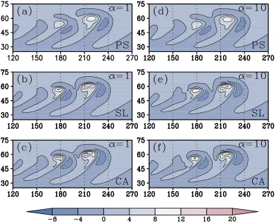
To begin with,Fig. 3presents the surface pressure at day 9 andng5128 resolution for the PS, SL, and CA

parametertis set to 2, 1 days for, respectively,a51, 10. For the PS algorithm, the diffusion coefficient is set in-dependent of vertical mode and so that the damping time for the shortest resolvable wave is 100 days, making the divergence damping virtually ineffective. The ref-erence solutions are given in Figs. 6 and 7 ofJablonowski

and Williamson (2006a). For the main body of the baro-clinic wave, that is, the two low–high pairs in the surface pressure with the corresponding feature in the 850-hPa temperature field (not shown), the solutions generally lie between the CAM finite volume solutions at 2:08 32:58

and 1:08 31:258resolutions. This is particularly the case

FIG. 2. Thel2([u]2[u0]) measure for the (a) PS, (b) SL, and (c) CA algorithms witha51,ng5128 (solid) anda51,ng5256 (dashed),

a510,ng5128 (dotted) anda510,ng5256 (dash–dotted).

FIG. 3. The surface pressure at day 9 withng5128 for the (a),(d) PS; (b),(e) SL; and (c),(f) CA algorithms for (left)

for the CA and SL solutions with a51, which have a stronger surface pressure disturbance than the solution witha510. The main deviation from the reference solu-tions is in the trailing and leading parts of the wave packet exhibited in the surface pressure field, precisely where there is also a degree of uncertainty in the four reference solutions shown in Fig. 7 ofJablonowski and Williamson (2006a). Compared with the reference solutions, there is also a reverse equator-to-pole pressure gradient that re-sults from the barotropic Rossby adjustment process tak-ing place because of the projection of small imbalance onto the barotropic mode.

The corresponding results for surface pressure at the higher resolution ofng5256 are shown inFig. 4. For the

SL and CA algorithms, the vertical-mode-dependent parameter t is set to 0:2, 0:1 days for, respectively, a51, 10. For the PS, the vertically uniform diffusion coefficient is set so that the damping time for the shortest resolvable wave is 10 days. What is most striking is the increase in amplitude of the baroclinic waves, making them closely comparable to the reference so-lutions. The main differences are again in the trailing and leading parts of the solutions and in the reverse equator-to-pole pressure gradient. To see that the

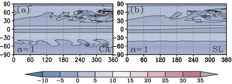
reverse pressure gradient is indeed a product of the initial imbalance, the corresponding results for the CA algorithms have been presented inFig. 5by initializing the zonally symmetric vorticity field using the balance relation(4.1). In this construction, for simplicity, in the right-hand side of(4.1)the analytic zonal velocity has been used, and the smaller nonlinear term due to vari-ation ofuonjsurfaces has been ignored.

To better understand how the surface pressure am-plitude varies with algorithm and resolution, the surface pressure minima and maxima over the domain att59 are given inTable 1. Fora51, the picture is clear. The smallest difference between the 1283128 and 2563256 solutions, the largest maximum, and the smallest mini-mum all come from the CA algorithm for which the extrema of (942:75, 1018:23) are closely comparable to the CAM Eulerian at T170 resolution, for which the corresponding extrema are (942:62, 1019:33) hPa. For a510, however, the picture is more complex. While the largest maximum comes from the CA algorithm at both resolutions (though with a small margin), the lowest minimum comes from the PS solution. The data for the reference solution of the CAM Eulerian were taken from the Atmospheric Dynamics Modeling Group at the

University of Michigan (http://clasp-research.engin.umich. edu/groups/admg/ASP_Colloquium.php).

Next we turn our attention to the 850-hPa relative-vorticity field at day 9 for which reference solutions have been given in Fig. 8 of Jablonowski and Williamson (2006a). It should be noted that unlike the smoother surface pressure field, there are substantial differences in the finescale structure of the waves among the refer-ence solutions at the peak of instability att59. Let us see how our algorithms perform atng5128 resolution

first (Fig. 6). The increase in amplitude by going from the PS to the SL and to the CA algorithms is evident. The PS solutions are also slightly ahead in phase with respect to the other solutions. Numerical experiments show that this phase shift comes from the action of the larger Robert–Asselin filter in the PS algorithm. Com-paring thea51 anda510 solutions, while there is little effect of the vertical coordinate in the PS algorithm, the higher amplitudes of thea51 solutions of the SL and CA algorithms are discernible. Further, the a510 so-lution has a phase lead of a few degrees with respect to the a51 solution. Together with the associated duction in amplitude, the above phase errors are re-sponsible for the higher deviation of thea510 solution from the reference solutions. Focusing on the CA solu-tions, the smaller amplitude of the baroclinic wave in the a510 solution is apparent in the two strong positive relative vorticity centers in thea51 solution, which it-self is generally comparable to the T85 spectral and the 1:08 31:258 finite-volume solutions presented in

Jablonowski and Williamson (2006b).

The corresponding solutions obtained usingng5256

resolution are shown inFig. 7. The remarks made on the comparison of thea51 anda510 solutions atng5128

remain valid. The near doubling of the positive relative vorticity centers make thea51 CA solution compara-ble to the T170 spectral and the 0:58 30:6258 finite-volume solutions presented in Jablonowski and Williamson (2006b). To better appreciate the impact of the algorithms, the domain values of minimum and maximum relative vorticity,z_minandz_max, respectively, are given inTable 2. Although not so evident att59, the impact of using contour representation in the CA emerges more clearly where the flow becomes more complex at later times. To demonstrate that, shown in

Fig. 8are the 850-hPa relative-vorticity fields at day 15 fora51 CA and SL algorithms. One can also see the earlier trigger of the Southern Hemispheric jet in-stability in the CA solution, which is a consequence of using the spherical geodesics in contour operations as remarked earlier.

With the visual inspection made inFigs. 3–8in mind, let us turn to some quantitative measures of the working of the PS, SL, and CA algorithms. The first measure is thel2norm of the difference between the solutions

ob-tained by these algorithms and the reference solutions for the surface pressure defined by

kp_s2p_s,refk₂5

2 6 6 4

å

i

å

(p_s2p_s,ref)2cosu_i,j

å

i

å

cosu_i,j 3 7 7 5

1/2

, (4.3)

FIG. 5. The surface pressure at day 9 withng5256 for the CA algorithm with (a)a51 and (b)a510. The balance relation(4.1)has been used to construct the initial vorticity field.

TABLE1. The extrema of surface pressure (hPa) att59. In each column, the first and second numbers are, respectively, for minimum and maximum values of surface pressure over the sphere.

Resolution PS21 PS210 SL21 SL210 CA21 CA210

where the sums are taken over all points of the half-grid used in the algorithms designed. The half-grid refers to a grid shifted by a half-grid interval in the meridional di-rection with respect to the poles. To determine(4.3), the reference solution is first interpolated to the half-grid using a fourth-order cubic Hermite interpolation. Using

(4.3), kp*s2p*_s,refk2 has also been computed, where p*s

denotes the deviation of the surface pressure from the zonal average. This is useful, askps2ps,refk2is largely

contaminated by the meridional noise arising from ini-tialization errors. The results of the PS, SL, and CA al-gorithms atng5256 resolution are presented inFig. 9,

where the reference solution is the spectral Eulerian solution at T170 resolution. When compared with the model intercomparison shown in Fig. 10 ofJablonowski and Williamson (2006a), until the buildup of baroclinic instability, the pressure difference between the solutions obtained and the reference solutions is more than an order of magnitude larger than the cross-model differ-ences inJablonowski and Williamson (2006a). However, when the contribution of the zonally averaged part of the solution is removed inkp*s2p*_s,refk2, the difference

field shown inFig. 9bbecomes close to the cross-model differences. Among the solutions shown, during the first 15 days of the simulation, the closest and furthest results to the reference solution come from, respectively, the CA algorithm with a51 and the PS algorithm with a510. For each of the PS, SL, and CA algorithms, the pressure differences are larger for a510. This obser-vation is related to the fact that the use ofa510 leads to a larger initial imbalance.

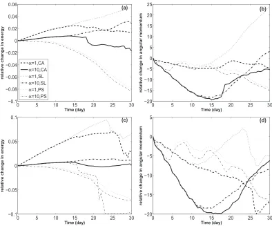
An examination of total energy [(3.20)] and angular momentum [(3.21)] gives us further information on the global conservation properties of the algorithms.

Figure 10shows the percentage relative changes in total energy, f[E(t)2E(0)]/E(0)g3100 and angular mo-mentum at ng5128, 256 resolutions. Overall, a wide

range of behavior is exhibited by the algorithms for the time variation in energy and angular momentum. At both resolutions, the two PS algorithms dissipate energy and angular momentum with a slightly higher rate for a510. For the SL algorithms, the buildup of energy during the 30-day integrations is considerably lower at

ng5256 resolution. Regarding angular momentum, except

for the generally increasing behavior seen fora51 at

ng5128 resolution, the remaining SL algorithms

ex-hibit oscillatory results. At both resolutions and for both vertical coordinates, the CA results are indistin-guishable from the corresponding SL results over the first 12–14 days of integration, that is, within the range of predictability of the flow (see Jablonowski and Williamson 2006a). Beyond around timet514, the CA results diverge strongly from the corresponding SL results, particularly so for energy ata510 and angular momentum ata51. It should be noted that atng5256

resolution, for a510 the application of the eighth-order filter in the zonal direction results in a substantial buildup of small-scale noise around the equator, lead-ing to numerical instability durlead-ing the second-half of the simulations. For this reason, the SL and CA results

fora510 shown here have been obtained by applying the eighth-order filter only in meridional direction to theh~field.

The relative changes in energy seen inFig. 10 may seem excessive. In the absence of results to compare to in the literature, we resort to indirect comparisons. First, a basic comparison can be made with the results presented in Fig. 4 of Mohebalhojeh and Dritschel (2007)documenting the variations in energy for various CASL algorithms applied to the test case ofGalewsky et al. (2004)for the spherical SW equations. The relative changes are well within the range of values seen in that test case. Second, another possible point of comparison is the 0:6 W m22_{estimate given inTaylor (2011)for the}

dissipation rate of kinetic energy, which is the main contributing factor to energy dissipation in aquaplanet

FIG. 7. As inFig. 6, but forng5256.

TABLE2. The extrema of relative vorticity (day21_{) att59. In each column, the first and second numbers are, respectively, for minimum}

and maximum values ofzover the sphere.

Resolution PS21 PS210 SL21 SL210 CA21 CA210

simulations by the CAM–High-Order Method Model-ing Environment (HOMME) model (Neale et al. 2012). To demonstrate the effect of overusing divergence damping (an extreme case of energy dissipation), also shown in

Fig. 10cis the result for the CA algorithm witha510 with a doubling of the vertical-mode-dependent damping. In this strongly dissipative case, we have E(t50)5 1:31273109_{J m}22_{,E(t530)51:3114310}9_{J m}22_{, and}

[E(t530)2E(t50)]/(30 days)5 20:5 W m22as a rough estimate for the average energy dissipation rate over the 30 days of integration. It is true that the instantaneous picture is much more complex, where bursts of dissipa-tion may be followed by larger periods of conservadissipa-tion. But overall, the average dissipation rate over sufficiently large time intervals can be expected to fall not far from the 0:6 W m22estimate ofTaylor (2011).

A further comparison can be made by quantifying the relative strength of the vortical flow in the CA solution with that in the PS and SL solutions. To this end, first the quantitiesC2andDdefined per unit area as

C₂51

2h(11h~)z

2_{i and (4.4a)}

D51

2h(11h~)j=zji (4.4b)

are computed for each 30-day integration. Hereh i de-notes the domain-area average over the Northern Hemisphere. Because of the earlier trigger of the southern hemispheric jet instability in the CA solution (Fig. 8), for a better assessment, the Southern Hemi-sphere has been excluded from the averaging. Taking the CA results at each resolution as the reference, the relative differences, like [C2(SL)2C2(CA)]/C2(CA) for

C2and SL, are then computed. The results witha51 are shown in Fig. 11. In both the C2andDmeasures, the

substantial reduction seen for the PS algorithm points to a dramatic underestimation of vortical activity with respect to CA. The overshoot in Dseen over the first 5 days of integration comes from a stronger generation of meridional imbalance in the PS solution. The SL

FIG. 8. The relative vorticity field at day 15 withng5256 anda51 for (a) the CA and (b) the SL algorithms.

FIG. 9. The quantitative measures of departure from the reference solution, taken to be that of the T170 Eulerian spectral model, forng5256: (a)kps2ps,refk2and (b)kp*s2ps*,refk2for the PS algorithm witha51 (red) anda510 (yellow), the

solution also suffers from a reduction of vortical activity, which is weaker than in the PS solution. There seems to be an exception to this statement because of the peak seen atng5256 around timet524. However, this arises

from the fact that vanishing layer thickness with a con-sequent generation of localized, large values of vorticity occur earlier in the SL solution.

Let us finally examine how the algorithms behave in terms of their kinetic energy spectrum at 700 hPa and

t530, for which results are available for the CAM finite volume dynamical core inJablonowski and Williamson (2011). Forng5256 resolution, spectra for the various

algorithms are presented inFig. 12. The main objective here is to highlight the effects of the varying damping procedures employed by the algorithms. The spectral slope between the total wavenumbers 10 and 100 is particularly sensitive to the degree of damping used for regularization of the flow and for numerical stability. The slope in the latter part of the spectrum can be compared with the referencen23_{distribution (Skamarock}

2011). This slope is closest ton23 _{for the CA algorithm}

witha51. Further, for each of the PS, SL, and CA al-gorithms, steeper slopes occur fora510. At the larger-scale end of the spectrum between the total wavenumbers 1 and 10, there is a significant scatter among the results in

Fig. 12as well as those in Jablonowski and Williamson (2011)for the CAM finite volume dynamical core. The scatter seen is much larger witha510. It is interesting to note that at this part of the spectrum, results close to the CAM finite volume dynamical core can be obtained, if the CA algorithm uses solely the sixth-order filter.

Computational cost

As an estimate of computational efficiency, the com-putational cost of the PS, SL, and CA algorithms are given inTable 3, relative to that of the low-resolution PS. Unlike the PS and SL algorithms, the computational cost of CA is heavily dependent on flow complexity. As the complexity substantially increases during the second half of integration, the relative costs have been given for

FIG. 10. The percentage relative changes in total energy and angular momentum for (a),(b)ng5128 and (c),(d)

ng5256. The results shown are for the PS algorithm witha51 (thin dotted) anda510 (thin dash–dotted), the SL algorithm witha51 (thick dotted) anda510 (thick dash–dotted), and the CA algorithm witha51 (dashed) and

the time intervals [0, 15] and [0, 30] days. When com-pared with the SL algorithm, the computational over-head of incorporating Lagrangian information in the CA algorithm is slight over the [0, 15] interval, but more than doubles over the [0, 30] interval. The latter sub-stantial increase comes from the finescale structures that are represented in CA and lost in SL. The impact of such structures, though not so evident in the quantitative measures presented, is expected to be greater in flows more complex than exhibited by the current test case.

5. Conclusions

The DCASL algorithms previously developed for the shallow-water equations and the hydrostatic Boussinesq equations have been extended to solve the spherical

hydrostatic primitive equations using a hybrids–u ver-tical coordinate. To this end, verver-tical modes have been formulated for the generalized coordinate by introduc-ing a variable called modified pressureP0that forms the linear part of the pressure gradient force. The DCASL algorithms solve the primitive equations in any of the (Q,d,g), (Q,d,P0), (Q,h~,d) representations where Q[(f1z)/(11h~) is a PV-like quantity and g[fz2=2P02buis an approximation to the horizon-tal acceleration divergence (=DhV/Dt). The

devia-tions of Q from the Rossby–Ertel PV and g from horizontal acceleration divergence result from the de-viation of the vertical coordinate from an isentropic one. Sufficiently far away from the lower boundary, asjtends tou,Qbecomes a close approximation to PV and thus the algorithm can be regarded as being PV based. The

FIG. 12. The kinetic energy spectra at day 30 and at 700 hPa for the PS (red), SL (green), and CA (blue) algo-rithms with (a)a51 and (b)a510. The resolution isng5256. The straight solid line gives the theoreticaln23 spectrum (see text).

FIG. 11. The relative differences in (a)kz2_k

2and (b)k=zk2between the solutions of the PS and the DCASL

algorithm with the prognostic variables (Q,d,g) in-volves an inversion problem to determine the depth and the thermodynamic fields. The inversion problem, however, turns out to be particularly difficult primarily because of the nonlinearity of the hydrostatic equation in thes–ucoordinate used. Except for theoretical models with a few layers, the resulting algorithm appears to be impractical. For the less demanding (Q,d,P0) algorithm, which is suitable for applying a semi-implicit scheme, an efficient and convergent method to determine thermo-dynamic fields fromP0has yet to be found. Therefore, for realistic models with a large number of layers, the focus has been on the (Q,h~,d) algorithm with an explicit time-stepping scheme. In addition to the problems with com-putational cost due to limitation to a short time step, it also turned out that the increased Lagrangian resolution on Q requires various types of damping, filtering, and regularization for computational stability.

Using the (Q,h~,d) algorithm, extensive numerical simulations have been carried out for the test case of baroclinic instability introduced by Jablonowski and Williamson (2006a). This is in fact a stringent test case for the DCASL algorithms developed, because the in-stability acts strongly at low levels near to the ground wherejdeviates fromu, and thus there are large sources of Qcoming mainly from vertical advection. The nu-merical assessment of the DCASL algorithm was un-dertaken together with two other algorithms derived from it: 1) the one called SL replacing the DCASL so-lution for Q by a standard semi-Lagrangian solution, and 2) an Eulerian algorithm called PS replacingQby z as the prognostic variable. Various degrees of im-provement from modest to significant over the SL and PS solutions at equal grid resolution were demonstrated. At medium horizontal resolutions, the DCASL algo-rithm can achieve results comparable to the reference solutions shown inJablonowski and Williamson (2006a,b). To address the convergence issue with the semi-implicit time-stepping scheme referred to above, work is under way on a modified algorithm that replacesP0by

P0_l, where P0_l is obtained by linearizing the right-hand side of(2.5), that is,

›P0_l

›j 5 P

0›u

›j2u

0›P

›j. (5.1)

With this change, it is possible to replace the column-wise iterative procedure(A3)by a procedure to solve a nonlinear equation separately for each layer from the bottom to the top of the model.

As a final remark, the need for various types of damping may be seen as the main deficiency of our working DCASL algorithm. To a certain extent, the problem with damping is related to the failure of our device to apply implicitly a form of balance relation, as in the (Q,d,g) algorithm, to control fictitious genera-tion of imbalance. Within the (Q,h~,d) algorithm, it seems that other methods to enhance the solution of the mass and divergence fields have to be found. This re-mains for future development of the basic DCASL al-gorithm presented here.

Acknowledgments.A.R.M. thanks the U.K. Natural Environment Research Council for a Research Fellow-ship, and the Universities of St. Andrews and Tehran for providing support during this research. Further financial support was provided by IR of Iran Meteorological Organization to which we are thankful. Special thanks also go to Sarmad Ghader, Mohammad Mirzaei, and Daniel Yazgi for their help in preparing the paper.

APPENDIX A

Procedure to InvertQ,d, andg

When the variablesQ,d, andgare used as the prog-nostic variables, one has to implement an inversion procedure to obtain the velocity field and the thermo-dynamic variables at each time step. Rewriting the definition of g as =2P05fz2bu2g, subtracting f2_h

from both sides, projecting onto the vertical-mode space, and dividing the result by c2

m, the following

modified Helmholtz equation is obtained:

=2₂f2 c2

m

h5 1 c2

m

f(z2fh)2bu2g zfflfflfflfflfflfflfflfflfflfflfflfflfflfflffl}|fflfflfflfflfflfflfflfflfflfflfflfflfflfflffl{

" #

. (A1)

It should be noted that the variable h defined by

h5C21Pis generally different fromh~. Equation(A1)is solved using the same method described inMohebalhojeh and Dritschel (2007)by spectral transform in longitude and

TABLE3. CPU time relative to the PS simulation at 128₃128 resolution. In each column, the first and second numbers are, respectively, for the first 15 and 30 days of the experiments.

Resolution PS21 PS210 SL21 SL210 CA21 CA210