ProFound: Source Extraction and Application to Modern
Survey Data
A. S. G. Robotham,
1
?
L. J. M. Davies,
1
S. P. Driver,
1
S. Koushan,
1
D. S. Taranu,
1
,
2
S. Casura,
3
J. Liske
3
1ICRAR, M468, University of Western Australia, Crawley, WA 6009, Australia 2ARC Centre of Excellence for All-sky Astrophysics (CAASTRO)
3Hamburger Sternwarte, Universit¨at Hamburg, Gojenbergsweg 112, 21029 Hamburg, Germany
Accepted XXX. Received YYY; in original form ZZZ
ABSTRACT
We introduce ProFound, a source finding and image analysis package. ProFound provides methods to detect sources in noisy images, generate segmentation maps iden-tifying the pixels belonging to each source, and measure statistics like flux, size and ellipticity. These inputs are key requirements ofProFit, our recently released galaxy profiling package, where the design aim is that these two software packages will be used in unison to semi-automatically profile large samples of galaxies. The key novel feature introduced in ProFoundis that all photometry is executed on dilated segmentation maps that fully contain the identifiable flux, rather than using more traditional circu-lar or ellipse based photometry. Also, to be less sensitive to pathological segmentation issues, the de-blending is made across saddle points in flux. We applyProFoundin a number of simulated and real world cases, and demonstrate that it behaves rea-sonably given its stated design goals. In particular, it offers good initial parameter estimation for ProFit, and also segmentation maps that follow the sometimes com-plex geometry of resolved sources, whilst capturing nearly all of the flux. A number of bulge-disc decomposition projects are already making use of the ProFoundand ProFitpipeline, and adoption is being encouraged by publicly releasing the software for the open source R data analysis platform under an LGPL-3 license on GitHub (github.com/asgr/ProFound).
Key words: methods: data analysis – techniques: image processing – techniques:
photometric
1 INTRODUCTION
Consistent and reliable source detection and photometric extraction has been a rich vein of research in astronomy. Clearly it is preferable to have a quantitative and repro-ducible means to analyse images, and over the years a num-ber of fully automatic tools have been developed to achieve such outcomes (e.g.Bertin & Arnouts 1996).
Our group recently developed the ProFit 2D galaxy profiling tool (Robotham et al. 2017), which requires a num-ber of reasonable inputs that require tools outside of the package. Critically important for achieving a good fit are: a pixel matched sigma map (reflecting the local uncertainty in the image provided); a segmentation map that flags the
? E-mail: [email protected]
pixels to use when computing the fit likelihoods; a careful sky subtraction; and reasonable initial guesses for the profile parameters.
A mixture of tools written in a number of languages cover most of the input requirements forProFit, however in practice how these tools are combined when scripting
ProFitfor a large automatic analysis of galaxy profiles has
a critical impact on how successful the fitting procedure is. With a particular focus on sky subtraction, object segmen-tation and initial parameter estimates (the three most diffi-cult aspects of galaxy profiling outside of the optimization problem itself) we developed the ProFound photometry package using theR data language (R Development Core Team 2016). Ostensibly this package is used to create good quality automatic inputs for further 2D decompositions with
ProFit, however it also serves as an extensively featured
source detection and photometric extraction package in its own right. ProFound is designed to work well with rel-atively deep large-area images where at least a significant minority (25+%) of the pixels belong to the sky, i.e. of the type that you might use for galaxy profiling. To combat im-age artefacts it supports the use of per pixel masks, but in general it works best of smoothly varying well calibrated images, i.e. images without serious pedestal mosaicking dis-continuities.
Blind source finding, as it is often known, has a long his-tory in astronomy (see the recent detailed review inMasias
et al. 2012, 2013). In the earliest days it was a
necessar-ily visual and heuristic process, where astronomers would identify sources in photographic images essentially by eye. As technology moved towards the era of digital detectors and large arrays of imaging pixels, computer techniques ad-vanced to automate these results in a more deterministic manner. Early techniques included simple sigma threshold-ing of the data in reference to the root mean square (RMS) fluctuations measured in the sky. This approach works well when the sources of interest are well above the sky noise. When sources move closer the surface brightness limit of the data, this technique can become increasingly ineffective, and lead to a higher than ideal false-positive rate. That is the number of new real sources can become subdominant compared to statistical fluctuations in the sky (Davies et al. 2005).
To combat this effect many improvements have been identified in the literature, e.g. simple schemes that smooth the data with an appropriate kernel and require a certain number of pixels to be above the RMS threshold and within a certain spatial separation on sky (seeSabatini et al. 2003, for a discussion on such techniques for uncovering marginally detected sources). In practice a matched filter is often the optimal smoothing kernel, where for convolution this is the transpose of the point spread function of the image (for the one dimensional matched filtering argument seeVan Vleck & Middleton 1946). Whilst these approaches are often ap-plied in an ad-hoc manner (e.g. the exact matched filter is often not chosen as the convolution kernel), they work well to qualitatively reduce the false-positive rate by essentially requiring a spatial correlation in image fluctuations, which reduces the chance sky noise fluctuations far below that im-plied by the threshold apim-plied.
Another area that is heuristic in nature but has been seen to work quite well in practice is source de-blending. This is a complex problem that is only satisfactorily resolved us-ing a full generative model, e.g. the 2D galaxy profilus-ing code
ProFit offers a mechanism for doing such an extraction.
However, in many applications this approach is prohibitively computationally expensive. A pragmatic option has been to process the image pixels with a source de-blending algo-rithm. These usually work on a variant of the so-called ‘wa-tershed’ de-blending. How these operate can differ in detail, but a generic feature is they separate the image into regions of distinct flux by approximating the image flux as belong-ing to different topographic structures, i.e. if the image was inverted these would approximately be seen as valleys (the positive flux sources) and flat noisy regions (the sky and the sky noise). If this topographic structure was steadily filled with water it is easy to see that structures that begin as distinct bodies of water will start to merge together as the
image becomes entirely flooded. There are various methods to use this insight to define genuinely distinct sources, but the basic approach is the same.
Mixed in with the above issues, there are a large num-ber of subtle effects that must be handled carefully. These include the sky estimation, the sky RMS estimation, and the growth of apertures to fully contain the flux. Each of these have long histories in astronomy literature, but they largely all share a heuristic approach. This is usually for pragmatic reasons of computational complexity rather than aiming to be the ideal solution in a demonstrative sense. The calculation of the sky and sky RMS are simpler problems to tackle for the most part (exceptions include very crowded fields and confusion limited data), and a large part of the Methods (Section 2) discusses the main approaches in de-tail. Choosing an appropriate method to fully capture the flux present is a more difficult problem to solve, and many approaches have been advocated in the literature.
The earliest attempt at systematically identifying the flux for extended sources can be found inPetrosian(1976). The basic idea behind the Petrosian magnitude is to deter-mine the radius to be scaled based on surface brightness properties of the galaxy, namely the ratio of the integrated surface brightness within some radius compared to the in-stantaneous surface brightness at the same radius. By incor-porating the surface brightness in the numerator and the de-nominator when calculating the Petrosian radius the results of many observational effects are naturally removed, e.g. cosmological surface brightness dimming, variable imaging depth of the data under consideration and different observ-ing conditions which can produce variable seeobserv-ing amongst other effects.
In theory the Petrosian magnitude is an elegant route to extract flux measurements, since in principle extracted extended source fluxes are not highly sensitive to the ob-serving conditions. In practice things are not as simple as we would like, and galaxies are not well represented as hav-ing a shared fundamental profile, which whilst not immedi-ately clear is implicitly assumed in the Petrosian magnitude system (Graham & Driver 2005). Since galaxies can have a very broad range of profiles the magnitude extracted is in fact highly sensitive to the profile S´ersic index (S´ersic 1963; Graham & Driver 2005). Since galaxies are also convolved with the atmospheric seeing in ground based data there is an additional dependence beyond the intrinsic profile, namely that the same galaxy shifted to higher redshift will return a different fraction of the true flux because the profile will have evolved away from its intrinsic value towards the at-mospheric value, which for a mixture of reasons is usually very close to a canonical S´ersic index of 0.5, i.e. a Normal distribution.
bySExtractor(Bertin & Arnouts 1996) is closely related to this version of the Kron magnitude, and can be run in such a mode that this multiplying factor is chosen intelli-gently for each source rather than using a single fixed value. A key feature of both of the above methods for extract-ing photometry is that they use either circular or ellipti-cal apertures. The earliest applications predominantly used circular apertures, with the elliptical variants being more modern and widely popular today. This suggests an obvi-ous limitation of either approach: galaxies are not simple ellipses, and decisions have to be made regarding how flux is distributed between potentially overlapping apertures.
The above motivated the most novel aspect of the
Pro-Foundcode presented in this paper: a move away from sim-ple elliptical apertures and towards apertures that properly identify the parts of galaxies containing the significant pro-portion of the flux. A few methods were looked at when first addressing this issue, with the result that dilated segments that follow the surface brightness distribution of the galaxies act as a better method to identify the true flux belonging to a given galaxy.
In the regime of bright compact elliptical sources, which are fairly isolated from other sources, the dilated segments follow the extent of traditional apertures fairly closely. How-ever, for very extended sources the differences can be quite pronounced, with complex source geometry not being accu-rately captured by simple circular or even elliptical aper-tures. The dilation approach also offers a few other advan-tages when it comes to source de-blending, namely that seg-ments are never allowed to overlap on the sky in the way the expanded apertures can. In fact it is non-trivial to deter-mine how best to split flux between adjacent and overlapping apertures, and a number of different ad-hoc and heuristic schemes are usually applied to account for these effects.
The hard flux boundaries created by using segmented apertures also have a number of advantageous side-effects when it comes to determining fluxes in regions that have pathological issues such as very bright halos around bright stars that have saturated the detector. These often create bi-ased photometry over an extended region, where the Kron or Petrosian aperture is often compromised and the expanded aperture overlaps with multiple fainter sources. We highlight some specific examples of this later in the paper, but it is a common feature of survey data (Wright et al. 2016). The method of iterative dilation used in ProFound naturally prevents extreme expansion artefacts since segments are not allowed to grow into each other. This is not to say the pho-tometry extracted will not be compromised at all, but the segmentation map and the approximate sources properties are much nearer to the intrinsic values and serve as better inputs forProFit, which was the initial design goal of the new software.
In Section 2 we describe the methodology behind the most critical aspects of the package design. In Section 4 we look at the application ofProFoundto fully simulated wide-field images, with a focus on the completeness and pu-rity of the detection, and the accuracy of the photometric properties. In Section5we applyProFoundto the UltraV-ISTA multi-band imaging data, with a detailed comparison of some of the output properties compared to the public catalogues.
2 METHODS
In the following description of the main methods behind
ProFoundsource extraction we use the same test Z-band
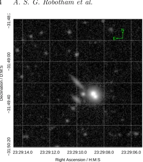
data shown in Figure 1. This was taken from the public VISTA (Visible and Infrared Survey Telescope for Astron-omy) Kilo-degree INfrared Galaxy (VIKING; Edge et al. 2013) survey that used the VIRCAM instrument on ESO’s 4m VISTA facility. The galaxy at the centre of the image was a main survey target (G5458748) for the Galaxy And Mass Assembly survey (GAMA; Driver et al. 2011; Liske et al. 2015). This image has a a number of properties that make it ideal as a small case study: it contains a mixture of bright and faint galaxies and stars; it contains a mixture of compact and extended galaxies, the central region contains a number of reasonably confused sources; the background root mean square (RMS) in the sky varies distinctly in the frame due to its stacked origin; and it has objects contained entirely within the image and near to the edge.
The example data is included with theProFound pack-age so it is easy for a new user to recreate the plots in this paper using the many worked examples and vignettes1. The thorough package documentation (the embedded PDF man-ual is 61 pages, with every function, variable and output de-scribed) and long-form vignettes have been influenced by the clear utility of the ‘SExtractorfor Dummies’ guide which has been hugely beneficial to the community who regularly useSExtractor(Holwerda 2005).
This paper is not intended as a user manual, so we will not discuss the technicalities of the detailed settings and pa-rameters here. Except where mentioned explicitly the code has been run in close to default mode, with the notable dif-ference being the setting of the magnitude zero point (which has to be set explicitly since there is no standard format to specify this in FITS headers). Otherwise meta-data is largely extracted from the FITS header and extraction properties are estimated dynamically using the data itself.
Functions in theProFoundpackage are all named with a leading lowercase ‘profound’. This is to remove the poten-tial for clashing function names since R does not trivially support package aliasing in the way that some high level languages do (e.g. Python). The ProFound package in-cludes a few different hierarchies of functions. The expec-tation is that some of these will be used routinely (e.g. the highest levelProFoundobject extraction and photometric measurement function, also called ProFound), and some will rarely be used by a typical end user (e.g. the linear interpolation functionInterp2D).
Between these two extremes there are a large number of mid-level functions that more advanced users might want to use directly in order to manipulate the data in a specific manner. The highest level ProFound function effectively links a large number of these mid-level functions together in a manner that achieves good quality source extraction and photometric analysis for a range of typical two dimensional astronomy data (particularly imaging and radio continuum data, but not limited to such applications). During develop-ment the focus has been on optical and NIR survey data, but it has also been used successfully on ultra-violet (UV) data and far-infrared (FIR) data.
23:29:14.0 23:29:12.0 23:29:10.0 23:29:08.0 23:29:06.0
−31:50:20
−31:49:40
−31:49:00
−31:48:20
Right Ascension / H:M:S
Declination / D:M:S
[image:4.595.45.274.79.339.2]N E
Figure 1.Example VISTA Z-band data taken from the VIKING survey included with theProFoundpackage and used in various parts of this paper (GAMA galaxy ID G5458748). In this Figure we stretch the z-scale to make the double star nature of the two bright central sources clear. In latter Figures we use a different mapping that enhances the contrast of fainter sources and visually merges these two stars together.
2.1 ProFound Source Extraction
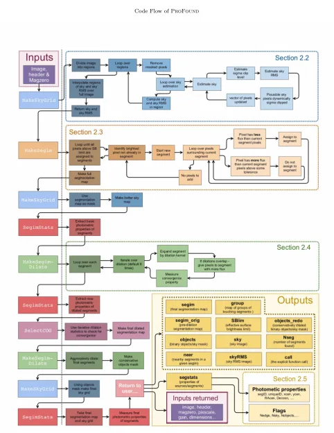
The highest levelProFoundfunction is ultimately a struc-tured calling of a range of mid-level functions. The full code diagram is presented in Figure 2with the various parts we discuss in more detail labelled by Section. The simplified version of Figure2 is provided below, where the mid-level function executed is named at each relevant stage.
(i) Make a rough sky map (see Section2.2) — MakeSky-Grid
(ii) Using this rough sky map, make an initial segmenta-tion map (see Secsegmenta-tion2.3) —MakeSegim
(iii) Using this segmentation map, make a better sky map —MakeSkyGrid
(iv) Using this better sky map, extract basic photometric properties (see Section2.5) —SegimStats
(v) Using the current segmentation map, dilate segments and re-measure photometric properties for the new image segments, by default it iterates six times (see Section 2.4) —MakeSegimDilate/SegimStats
(vi) Using the iterative dilation statistics, every object is checked for convergence, by default convergence of flux is used (see Section2.4) —selectCoG
(vii) Make final segmentation map by combining the seg-ments when each source has converged in flux
(viii) Make a conservative object mask by aggressively dilating the final segmentation map —MakeSegimDilate
(ix) Using this conservative objects mask make a final sky
map —MakeSkyGrid
(x) Using the final segmentation map and the final sky
map compute the final comprehensive photometric proper-ties —SegimStats
(xi) Return a list containing the input image pixel-matched final segmentation map (called segim), the pre-dilation segmentation map (segim orig) , the binary ob-ject/sky mask (objects), the conservatively dilated binary object/sky mask (objects redo), the sky image (sky), the sky-RMS image (skyRMS) and the effective surface bright-ness limit image (SBlim)
(xii) Return the data-frame of photometric properties for every detected source (segstats)
Some other simple properties are passed through and included in the output of ProFound: the original image, the image header (header) if it is attached to the input image, the magnitude zero point specified (magzero), the gain in electrons per astronomical data unit (gain), the pixel scale in arc-seconds per pixel (pixscale) and finally the full func-tion call (call).
The above detection and extraction sequence was de-veloped on a range of test data, where the desire was that good quality results should be achievable when running on default parameters. The latter was deemed important since parameter tuning can be non-obvious and complicated for novice users. Even in examples where qualitatively better extraction could be achieved by changing the parameters away from defaults, the changes were usually small and the impact marginal (i.e. pathological failure is very rare).
The emphasis during development was on robustness rather than speed. E.g. as written the sky determination is a relatively expensive operation, and by default this is done three times with increasingly aggressive object masks in or-der to be robust against biases due to extended objects and crowded fields. Even with the iterative object dilation and sky subtraction routines turned off,ProFound is still no-tably slower and more memory intensive thanSExtractor (Bertin & Arnouts 1996), typically a factor of a few slower for the same data when achieving a similar number of source extractions. Since it is largely written inRin a highly func-tional manner, there is a lot of data copying between differ-ent levels of functions, although efforts are made to minimise this whilst still preserving the safe and functional nature of R code.
Code Flow ofProFound
A limitation compared to SExtractor is that the main ProFound function cannot natively handle matrix-like images much larger than 46k×46k pixels (strictly a hard limit of 231−1 pixels in total), even on machines with much more memory available. A higher-level function (
Pro-FoundLarge) is included to process very large FITS files, which extracts overlapping subregions directly from a target FITS file, and recombines them in an unambiguous manner. The UltraVISTA survey data discussed later in this paper was processed using the ProFoundLarge function since it is marginally too large to be extracted in a single pass and served as useful test data, although the sub-region of interest for the Deep Extragalactic VIsible Legacy Survey (DEVILS; Davies et al. in prep) is ultimately smaller than the231−1pixel limit. A reason to take this approach is that
ProFoundLarge can compute the data in an embarrass-ingly parallel manner, whereas most of the routines within
ProFoundare inherently single-threaded in nature. Routes exist to compileRwith support for multi-threading, but this requires reasonably advanced knowledge, and our assump-tion is most users ofProFoundwill be using the standard single-threaded version ofR.
For a typical survey image run with default parame-ters the various stages take fairly predictable proportions of the total computing time: calculating the full watershed de-blend for the segmentation map dominates the total time (∼50%), followed by calculating the sky map (done three times by default,∼20%), iteratively dilating the image seg-ments (done six times by default,∼20%) and calculating the photometric properties of the segments (done once per di-lation step and again at the end, so seven times in total, ∼10%). Since the watershed stage dominates the time and uses an efficient external function written in C, the potential optimization gains are quite moderate. Reductions in pro-cessing time are possible if the number of sky calculations and/or the number of dilations are reduced from the de-faults. When run in matched segment mode the processing time is significantly reduced since the watershed de-blend stage is no longer required. If the sky subtraction and di-lation steps are also turned off then the total processing time can be reduced by a factor ∼10, i.e. the minimum re-quirement is that photometric properties of the provided segments are computed.
2.2 Sky Subtraction
An important step in almost any approach to object extrac-tion from astronomical imaging data is the sky subtracextrac-tion. Depending on the origin of the data the image might arrive to the user fairly flat and featureless in the background (e.g. optical drift scan data with the Sloan telescope;Ahn et al. 2014) or complex and variable at a number of different scales (e.g. near-infrared data with variable fringing artefacts; An-drews et al. 2014).
Given the potential complexity of the sky background it is rarely sensible to attempt to construct a formal statisti-cal model of the sky since it is very difficult to meaningfully parameterise the range of behaviour observed (see Bijaoui
1980;Irwin 1985). Instead most popular astronomy
applica-tions have taken the route of a heuristic but visually appeal-ing and pragmatically achievable scheme: coarsely sampled sky measurements combined with a polynomial interpolation
(Bertin & Arnouts 1996). Key parts of this process are that
truesky pixels need to be identifiable in the target image, and some manner of estimating their variance and absolute level is possible.
The above is achieved in a practical manner by clipping likely objects out of the data and using a sliding box car filter on a grid to measure image properties. With a meaningful sampling of the sky and sky-variance a traditional scheme to interpolate between grid points (e.g. bilinear or bicubic) can then be used to construct a per-pixel estimate of the sky. The caveats to this process are that objects need to be well masked (else they will systematically bias the estimators) and the box car scale has to be well chosen so as to remove the real sky variations and not structure that belongs to objects in the image. The sky is extrapolated at the edges, which can cause artefacts if it is changing rapidly and bicubic interpolation is used. In this scenario bilinear interpolation is the safer option since it does not use higher order polynomial terms that cause this effect.
The main high-level sky estimation routine in Pro-Found (MakeSkyGrid) allows users to pass an image,
masks (both for flagged pixels and for identified objects), the box car size, the grid sampling and the type of sky in-terpolation to use (bilinear of bicubic). This fairly simple functional interface allows for a large amount of flexibility in usage. The default code flow is as follows (names of the
Rfunctions used are displayed in small caps):
(i) Divide the image into regions based on the requested box car and grid sampling. By default the grid sampling inherits the box car size, meaning pixels are evaluated once (ii) Each sub region is analysed separately in a large loop:
(a) The masked pixels are removed from analysis, leav-ing a vector of fiducial sky pixels (skyf id−pix)
(b) Then the following is computed iteratively (either until the clipping is converged, or after 5 iterations):
(1) The sky value is estimated as sky =
median(skyf id−pix)
(2) The dynamic sigma clip level is estimated to be σcli p=qnorm(1−2/Nsky)
(3) The standard deviation of the sky pixels is estimated as skyR M S = quantile(skyf id−pix,0.5) −
quantile(skyf id−pix,0.159)
(4) The plausible sky pixels are dynamically sigma clipped such that pixels satisfying skyf id−pix > sky+
skyR M Sσcli p∨skyf id−pix<sky−skyR M Sσcli pare re-moved
(5) The vector of skyf id−pix is updated and these new fiducial sky pixels are used for the next iteration
(c) Once convergence has been achieved the final com-putedskyandskyR M S values are returned for the region under consideration
(iii) With all regions having a unique estimate of thesky
and skyR M S a bilinear or bicubic interpolation scheme is used to calculate plausible sky and skyR M S values for all pixels
As discussed above, the sky is measured a number of times duringProFoundsource extraction. The basic design philosophy is that it is possible to measure more accurate values for the sky and sky RMS as the objects are extracted, leaving behind increasingly certain sky pixels, more accurate identification of true sources, and better photometric mea-surements of the segments.
2.2.1 Different Sky Estimators
In principle the clipping process works on positive and nega-tive pixels, but unless there are serious artefacts in the data it will work predominantly on the positively valued pixels by removing undetected and un-extracted sources. The clip-ping process can be changed so as to not clip out possibly biased pixels, and the type of estimator for the sky can also be changed from median to mean or mode. Whether or not these options are used depends on the type of image be-ing analysed, and what the aim of the source extraction is. An implicit assumption in ProFound (and indeed
SEx-tractor) is that the sky fluctuations are symmetrically distributed around some intrinsic value. This will only be true in detail when the number of sky photons is fairly large (many dozens or more) and we can use the Normal∼Poisson approximation.
The difference between the sky level estimators (most commonly the mean, median or mode) and sky RMS level estimator (e.g. quantile versus standard-deviation) is an in-teresting point to consider. In the toy situation described it is preferable to use the mode (or possibly median if the mode is noisy and/or poorly sampled) for the sky and the quantile for the sky RMS, since these are both systemati-cally nearer to the specified ‘intrinsic’ sky for these simple estimators (Irwin 1985). However, what really matters is the origin of the positively biased flux that skews the distribu-tion. There are a number of processes that generate the ‘sky’ and contribute to the extended area signal in a typical digital detector image, in roughly descending order of importance:
(i) The actual night sky caused by Earth’s atmosphere glowing. Can be quite spatially and temporally variable (e.g. NIR images, distant artificial lights turning on and off)
(ii) Flux scattered around the image due to telescope op-tics or instruments producing scattered light and/or very broad∼Lorentzian wings
(iii) Scattering of astronomical light by the Earth’s at-mosphere, usually at very small scales (close to Gaussian usually)
(iv) Intrinsically broad features caused by the Milky-Way’s foreground cirrus
(v) Intrinsically broad wings caused by extra-galactic sources (e.g. the low surface brightness wings of galaxies or intra halo/cluster light)
(vi) Undetectable faint compact sources, can be struc-tured (Milky-Way stars) or effectively uniform in distribu-tion (high redshift galaxies)
The question is then: which of these do we wish to re-move? The answer clearly depends on what sources we are trying to extract photometry for. If we are measuring stellar photometry of a bright star then we almost certainly want to remove 1/4/5/6, i.e. we want to model the light from the star that has been scattered by the atmosphere and the
telescope (assuming it is the dominant contribution close to the star being modelled). If we want to profile a faint galaxy then you probably need to remove 1/2 (assuming it is mostly caused by other sources)/3 (assuming it is mostly caused by other sources)/4/6, i.e. we want to keep the faint wings of the target galaxy intact. There is not a trivially right an-swer, but ProFound does offer a few routes to compute these different types of sky which are described at length with examples in some of the available vignettes2.
In summary, aProFounduser might reasonably prefer a median, mode or mean type sky, depending on the use case. If the source sits on top of the sky (whatever makes it) then the user probably wants to use the more biased mean estimator. If the source is the dominant part of the observable background (e.g. when profiling the faint wings of galaxies) then the user might prefer the less biased median or mode estimators and more aggressive source clipping.
A final issue is whether you can extract better galaxy profile models by also using ProFit to model the back-ground for a given source, whereProFit has the capacity to model a flat local floor for the sky. The three obvious options are:
(i) UseProFoundsky subtraction on the image and do not fit a sky background inProFit
(ii) UseProFoundsky subtraction on the image and also fit a sky background inProFit
(iii) Do not use the ProFound sky subtraction on the image and only fit a sky background inProFit
For pragmatic reasons of needing to remove complex sky that cannot be fully generatively modelled withProFit, options (i) or (ii) are likely to be the best strategy for the majority of use cases.
2.3 Segmentation Map
Due to the emphasis on making segmentation maps that are useful inputs for ProFit galaxy profiling, the method of making segmentation maps differs in important ways to the method used in Bertin & Arnouts (1996) (i.e. SExtrac-tor, which in turn was inspired by Beard et al. (1990)). The most significant practical difference is that pixels that are flagged as being above a requested surface brightness threshold (be that stated in terms of sky RMS fluctuations or absolute surface brightness) are de-blended using a non-discretised watershed algorithm that creates flux de-blends through two-dimensional saddle-point cuts in image space, rather than one-dimensional cuts in flux space. The water-shed approach outlined here is nearest in spirit to the ‘FO-CUS’ de-blend method ofJarvis & Tyson(1981) and vari-ants of the popularMeyer (1994) ‘priority flood’ algorithm
(seeZhang et al. 2015;Zheng et al. 2015, for recent
astro-nomical applications).ProFounduses the iterative process outlined below:
(i) Identify the brightest pixel in the image above the specified surface brightness level which is not already as-signed to a segment
(ii) Progressively search unassigned image pixels sur-rounding the current segment, for each pixel searched:
(a) If a searched pixel has less flux than any neighbour-ing pixels already assigned to the segment, then assign to the current segment if no unassigned pixels neighbouring the pixel under consideration have more flux
(b) If a searched pixel has more flux than its neighbours already assigned to the segment above some tolerance level then do not assign it to the current segment
(c) If no more pixels can be assigned to the current segment then terminate the growing process
(iii) Select the next brightest unassigned pixel remaining in the image and assign it to a new segment, then repeat the above segment growing process
(iv) Once all pixels above the specified surface brightness level have been assigned to a segment terminate the water-shed process
There are a small number of parameters that have a significant effect on the watershed process, and in practice these need to be slightly altered to best segment the data under consideration. The most important is the ‘tolerance’, which specifies to what degree pixel growth is allowed to traverse uphill within a segment. In practice this determines the level of de-blending between closely separated flux peaks, where a higher tolerance means less splitting up of extended regions of flux. This is always specified in terms of the RMS of the sky and is 4 by default, i.e. a fluctuation would need to be more than 4 deviations of the sky RMS above the neighbouring segment pixel in order to not be included as part of the current segment being grown. The next most important parameter is the smoothing applied to the image (sigma), where by default a Gaussian kernel with a standard deviation of 1 pixel is used to blur the image. The smooth-ing can be turned off entirely, but this is rarely a good idea since there is always a large degree of pixel-to-pixel noise in all but most correlated images (typically flux values only appear smooth on the scale of a few pixels). Instead it is sometimes justifiable to increase the smoothing size, with an upper limit of 3 or 4 sometimes more suitable for images of large well-resolved galaxies. Related to this is the ‘ext’ parameter which is passed directly to theEBImage water-shed function used in ProFound (Gregoire et al. 2010).
This determines the allowed search radius around each pixel (rather than restricting the search to immediately adjacent pixels), where the default is 2 pixels. The smoothing ‘sigma’ and the search radius ‘ext’ have a similar impact and small changes in at least one of them (over the range 1–4) are com-mon when first applyingProFound to a new dataset and tuning for optimal segmentation. Increasing the smoothing is an effective strategy for extracting extended low surface brightness sources.
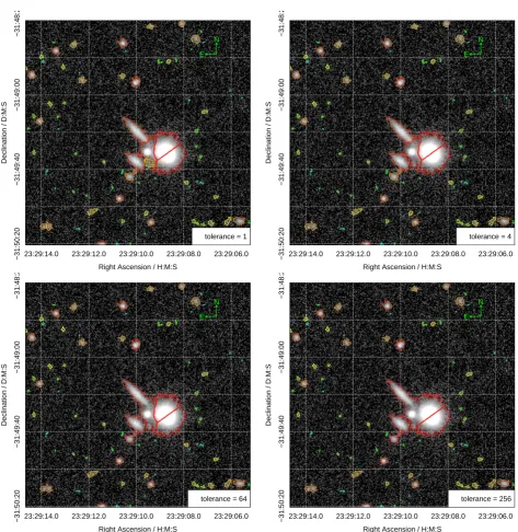
Figure3demonstrates how the de-blender used in Pro-Found works in practice for different watershed tolerance
levels. The main consequence of using the above approach is that islands of segments within larger segments can never be created. Instead the de-blended segments reflect the seg-ment water would flow into if the flux map was turned upside down (ignoring dynamical effects like momentum, and just specifying the pixels that water would next flow into if the velocity was set to zero). There are other definitions of
‘wa-tershed’, but this is the most standardised in the field of geology and accurately reflects a true gravitationally influ-enced watershed map. An internal Sloan Digital Sky Survey memo discusses the relative merits of different de-blending approaches3, with the general remark that all approaches make compromises and assumptions. This is true even for full generative modelling, given the requirement to define the parameterization of the model.
For our stated aims of producing good segmentation maps for passing intoProFit, the type of saddle point seg-mentation discussed above works well since it errs on the side of ignoring pixels compromised by nearby sources when modelling the profile of a target galaxy. Qualitatively we also see relatively few occasions of segments being grouped together in a common aperture erroneously, which we some-times see to occur when runningSExtractor(seeWright et al. 2016, and the UltraVISTA example below for examples of such situations).
The fullProFitmodel of the central complex shown in Figure3yields photometric properties (most notably flux) not far removed from theProFoundestimates (less than 0.5 mag differences). However, it is in general more important to get the correct number of segments and mode locations than having very good initial estimates for the fluxes and sizes. This is because estimating the number of components and mixtures is more difficult when galaxy modelling than opti-mising the parameters of a given model. WhilstProFound
does include routines to improve object measurements based on symmetry and flux sharing, these are turned off by de-fault since they are computationally costly and generally unnecessary (i.e. the raw measurements are good enough).
The underlying code that computes the watershed de-blend comes from the image processing packageEBImage
that is already available inRand widely used for low-level image processing (Gregoire et al. 2010). Its design and fo-cus was for cellular biology (the EB in the name standing for European Bioinformatics) where the main task tackled was how to correctly segment images of cells taken by mi-croscopes. As often noted anecdotally, there is much similar-ity between an image of biological systems and astronomy images, the former probably being the more complex to or-ganise and segment in a systematic manner. For this reason it is not surprising that a tool developed for such an ap-plication works well for astronomical images. An important feature of the routine used is that it does not discretise the flux levels in the image (as SExtractor does) and uses the full flux resolution available. This fact means that it is quite slow (despite the underlying code being written inC), and the watershed step usually dominates the computation time for larger images since it scales as O(nlogn) whereas nearly every other subroutine scales asnor better (wheren
is the number of pixels in the target image). The effect of this is that it can be faster to runProFoundon sub-regions rather than one very large image. It is only beyond the size of 10k×10k images (more than108pixels) that the difference becomes worth considering.
For convenience when using the outputs ofProFound the identities of neighbouring segments with respect to all other segments and also the friends-of-friends groups of
23:29:14.0 23:29:12.0 23:29:10.0 23:29:08.0 23:29:06.0
−31:50:20
−31:49:40
−31:49:00
−31:48:20
Right Ascension / H:M:S
Declination / D:M:S
N E
tolerance = 1
23:29:14.0 23:29:12.0 23:29:10.0 23:29:08.0 23:29:06.0
−31:50:20
−31:49:40
−31:49:00
−31:48:20
Right Ascension / H:M:S
Declination / D:M:S
N E
tolerance = 4
23:29:14.0 23:29:12.0 23:29:10.0 23:29:08.0 23:29:06.0
−31:50:20
−31:49:40
−31:49:00
−31:48:20
Right Ascension / H:M:S
Declination / D:M:S
N E
tolerance = 64
23:29:14.0 23:29:12.0 23:29:10.0 23:29:08.0 23:29:06.0
−31:50:20
−31:49:40
−31:49:00
−31:48:20
Right Ascension / H:M:S
Declination / D:M:S
N E
[image:9.595.54.528.91.578.2]tolerance = 256
Figure 3.Examples of using different watershed de-blend tolerance levels on the initial segmentation map, as per labelled on each panel. There is no truly objective approach to say which solution is preferred, but most professional astronomers would probably suggest the best answer lies in the regime of tolerance 1–4, where the central confused complex has been broken up into its plausible sub-components.
blended regions can also be returned. The latter is par-ticularly important when usingProFound as an input to
ProFit, since you should minimally try to fit all the seg-ments in a grouped friends-of-friends region when trying to profile blended objects. These two types of grouped struc-tures are not trivially returned bySExtractor, so for cre-ating profiling inputs this is a clear advantage of using
Pro-Found.
2.4 Segment Dilation
The next phase of the source extraction routine grows the segments using circular top-hat (by default) dilation
opera-tions until convergence has been achieved. As highlighted in the introduction, the segment dilation method is the most novel aspect of howProFound operates. At no stage are fluxes or object properties calculated using apertures (be they circular or elliptical). Instead all integrated properties related to the source are estimated using the dilated seg-ments alone. The procedure is iterative and therefore rel-atively expensive compared to simply expanding the inner Kron or Petrosian radius by some factor that approximately contains a large fraction of the flux.
seg-0 1 2 3 4 5 6
0
0.05
0.1
0.15
0.2
0.25
0.3
0.35
Iterations Required for 5% Flux Convergence
Stars Galaxies
Figure 4. Histograms of the number of iterations required to reach flux convergence for both stars and galaxies. The data is taken from the large suite of simulations that we discuss in Section 4.
ment being grown has converged and the dilation should stop. Figure4shows the required number of dilation itera-tions before flux convergence is achieved for a large suite of simulated data containing 40k stars and galaxies that we dis-cuss in detail later. It is notable that typically stars require fewer iterations than galaxies in order to achieve the default level of convergence (5%). The minimum number of itera-tions is zero, but only a very small fraction of stars require so few dilations. More typically stars require two dilations and galaxies require four.
The dilation distribution has not fallen to zero for stars, and more clearly galaxies, even by iteration six. This sug-gests that galaxies in particular have such extended flux en-velopes that they need even more dilations. It is possible to increase the maximum allowed number of dilations to greater than six, but this was considered to be a sensible compromise default value. The sources requiring six dilations are notable for having the lowest integrated surface brightness levels of all sources (i.e. these are the most marginal detections), so the danger of pushing to much more aggressive dilation lev-els is that a significant amount of noise is incorporated into the aperture, compromising the photometric properties of the object being measured.
With the main design considerations for the segment dilation process now justified, the basic flow is as follows:
(i) Execute a number (the default is six) of dilation oper-ations on all segments, for each dilation operation:
(a) Expand every segment with a dilation kernel (by default this is a circular top-hat with a diameter of nine pixels)
(b) If segment dilations overlap then give all pixels to the segment containing more flux in the current iteration (c) Measure the convergence property of interest for the new dilated segmentation map (by default this is the flux)
(ii) After all dilations have been made look through all segments and determine when each segment has converged within some tolerance (this is within a factor 1.05 in flux by default)
(iii) Put these converged segments together to make a final dilated segmentation map
The dilation operation is executed by thedilate func-tion in theEBImagepackage. This is optimised in design for detecting the full extent of pixels belonging to an al-ready labelled biological cell. A useful feature ofProFound is that it can accept any segmentation map as long as it has the generic feature that the segments are non-zero integers and the sky is labelled as 0. This means it is perfectly possi-ble to pass in a segmentation from another software package (e.g.SExtractor) and then useProFoundto execute the dilation and flux convergence algorithms.
There is trade off to be made between setting the ini-tial detection threshold of the image higher and allowing a larger number of more aggressive dilation operations, but the key point is that at least three (by default) pixels must be identifiable as a segment above the detection threshold in order to even be dilated. The default parameters work well on a range of common survey imaging data (e.g. SDSS (Ahn et al. 2014), KiDS (Kuijken et al. 2015), VIKING), so the need for large deviations from the defaults should be rare. In fact the settings related to the dilation operations are almost never altered in normal usage.
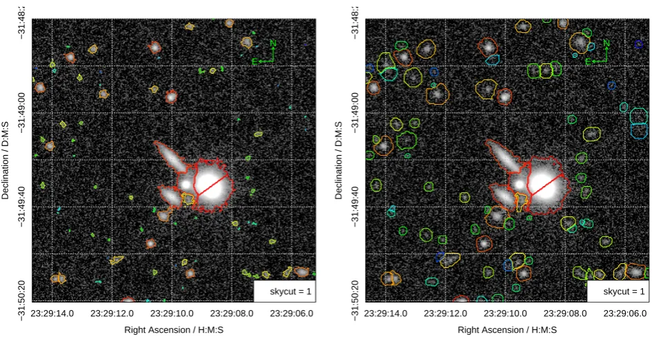
Figure5shows the segments that define the bright ini-tial components of the segmentation maps and the fully dilated segments for the same objects. Comparing the un-dilated segments (left panel) and the un-dilated segments (right panel) it is clear the bright stars do not dilate much be-fore their flux converges, but fainter extended galaxies grow much larger in order to capture their converged share of flux. It is also notable that the geometries of the segments are kept largely intact during dilation.
Internally the dilated segments are used to compute a number of traditional geometric parameters such as effec-tive size and ellipticity of the segment were it forced to be an ellipse. The approximate semi-major axis is output as ‘R100’ inProFound, where the ratio between this and the standard Kron aperture (which is computed using the first order moments of the pixels in each segment) can be thought of as the expansion factor, which tends to be set to values between 2 and 4 when using aperture based photo-metric tools. Rather than being specified this is measured inProFound. Figure6shows the typical factors for a suite of simulated VIKING depth data (introduced and discussed in more detail later in this paper). It is clear there is an absolute lower limit near to two, and only the very bright-est stars and galaxies require expansion factors beyond four. The discreteness seen for the stars is a consequence of the iteration process, where the thickest branch contains stars that require two dilations for convergence, as seen in Figure 4.
23:29:14.0 23:29:12.0 23:29:10.0 23:29:08.0 23:29:06.0
−31:50:20
−31:49:40
−31:49:00
−31:48:20
Right Ascension / H:M:S
Declination / D:M:S
N E
skycut = 1
23:29:14.0 23:29:12.0 23:29:10.0 23:29:08.0 23:29:06.0
−31:50:20
−31:49:40
−31:49:00
−31:48:20
Right Ascension / H:M:S
Declination / D:M:S
N E
[image:11.595.54.527.96.342.2]skycut = 1
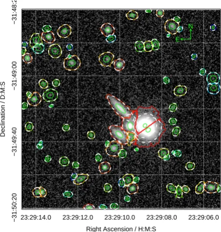
Figure 5.An example of the default diagnostic output from the mainProFoundsource extraction routine using the example VISTA Z-band data taken from the VIKING survey (as shown in Figure1). The left panel shows the identified flux (non-dilated) segments via multi-coloured contours (red showing the brightest sources, via green, through to blue showing the faintest). The right panel is similar, but the contours now represent the fully dilated and flux converged segments. The left panel is actually identical to the top-right panel in Figure3, but it is repeated here to aid direct comparison of pre and post dilation.
has de-blended through multiple saddle points. Since these segments will have necessarily non-elliptical geometry there is no good elliptical approximation for the segment regions. Since the elliptical apertures are not used to compute pho-tometry withinProFoundthis is not a concern to people using the software in an isolated fashion, but it does mean that care has to be taken when attempting to apply these apertures using other programs (e.g. LAMBDAR Wright et al. 2016).
2.5 Photometric Properties
Once a segmentation map has been constructed a sepa-rate internal function is used to calculate a large suite of photometric properties and segment flags. Internally this is achieved by associating all pixels with their respective seg-ments, looping through each segment, extracting the rele-vant pixels for the current segment, and computing photo-metric properties using just the pixels flagged as belonging to a particular segment. To achieve this process rapidly
Pro-Founduses the highly efficientdata.tablepackage4which is optimised for subsetting and processing on large datasets. The main photometric properties returned are listed in Table1(ignoring the various types of flags, alternative def-initions of some quantities, and error columns). These out-puts are sufficient to provide reasonable initial guesses for a single S´ersic profile fit of a galaxy usingProFit, which was the main initial design focus for ProFound. The as-sumption is that a multi-component profile will be built in complexity iteratively, i.e. in order to achieve good inputs
4 https://CRAN.R-project.org/package=data.table
for a two component fit you would first start with a simple single component fit.
ProFounddoes not execute sophisticated algorithms
to de-blend flux between neighbouring sources/segments. In comparison, methods presented inIrwin(1985) (simultane-ous maximum likelihood of sources) andBertin & Arnouts (1996) (heuristic flux division via symmetry expectation) do. In order to extract truly optimal photometry the iden-tified blended sources should be further run through gener-ative modelling software such asProFit(e.g.Kelvin et al.
2012, see Section 3for an example). However,ProFound
includes a number of schemes to flag and improve photom-etry in complex and confused regions. Improved flux re-construction is possible using the ‘rotated’ flux output for sources (‘flux reflect’ and ‘mag reflect’ in Table 1), which assumes flux symmetry of sources. This option determines a plausible amount of missing flux by rotating each segment about the central pixel and determining how much flux does not fall onto a mirrored segmented pixel. Running on the VIKING example data, the median difference between the raw segment flux and the rotated version is∼0.1 mag (i.e. the sources get brighter), so for most sources the difference is fairly small. The scale of these differences is also in line with the kind of flux differences seen when attempting full profile modelling withProFit(see Section3).
ProFoundalso returns a large number of flags that can
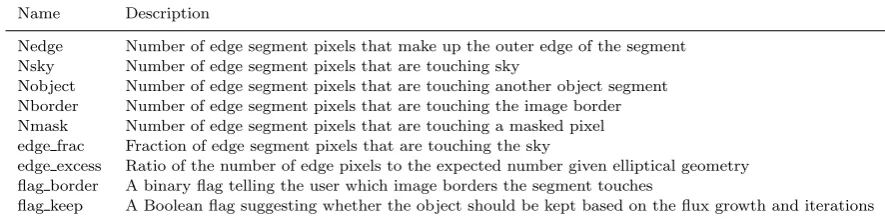
Table 1.A selection of photometric properties computed inProFound
Name Description
segID Segmentation ID uniqueID Unique ID
xcen Flux weighted x centre ycen Flux weighted y centre
RAcen Flux weighted Right Ascension centre Deccen Flux weighted Declination centre flux Total flux in the segment in ADUs
mag The flux in the segment scaled to a magnitude
flux reflect Total flux in the segment in ADUs scaled by flux missing under a segment rotation mag reflect The flux reflect in the segment scaled to a magnitude
N50/90/100 The number of pixels containing 50% / 90% / 100% of the flux
R50/90/100 Approximate elliptical semi-major axis containing 50% / 90% / 100% of the flux SB N50/90/100 Mean surface brightness containing 50% / 90% / 100% of the flux
con The concentration, defined here as R50/R90. axrat Axial ratio of ellipse
ang Orientation angle of the ellipse
Table 2.Flags and diagnostics computed inProFound Name Description
Nedge Number of edge segment pixels that make up the outer edge of the segment Nsky Number of edge segment pixels that are touching sky
Nobject Number of edge segment pixels that are touching another object segment Nborder Number of edge segment pixels that are touching the image border Nmask Number of edge segment pixels that are touching a masked pixel edge frac Fraction of edge segment pixels that are touching the sky
edge excess Ratio of the number of edge pixels to the expected number given elliptical geometry flag border A binary flag telling the user which image borders the segment touches
flag keep A Boolean flag suggesting whether the object should be kept based on the flux growth and iterations
be compromised by nearby sources unless effort is made to execute a model that also accounts for these sources.
2.6 Colour Photometry
Colour photometry is a catch-all term that usually refers to measuring fluxes in multiple bands using common aper-tures, where the differences in fluxes can be mapped onto traditional optical colours for visualization purposes. The higher levelProFoundfunction that provides the main in-terface to both source extraction and photometric analysis offers a few routes to extracting colour photometry. The top level interface can take a number of inputs that bypass inter-nal routines to calculate them, e.g. segmentation maps, sky maps and object masks. Since the image provided does not have to be the same as the one used to create the segmenta-tion map provided, it is easy to extract forced photometry by passing intoProFounda pixel matched image that was observed using a different filter to the detection band, and turning off the option to dilate the segments.
A more advanced method, useful in the case where the point spread function (PSF) varies significantly between bands, is to allow the segments to dilate to best extract con-verged flux in the target band. This is referred to as soft colour photometry inProFound, and is a sensible method to extract total photometry across multiple bands with dif-ferent depths and seeing conditions. In general the highest
image quality and/or deepest band should be used as the detection image. Additionally,ProFoundincludes routines to optimally stack images based onS/Nproperties, in which case a stacked image can be used as the detection image (this was used for the UltraVISTA data analysis presented in Section5).
One issue is that the above methods require the images to be pixel matched. TheProFoundpackage includes rou-tines to remap images onto a common target Tan-Gnomonic world coordinate system (WCS), should the images not have a common projection. To do this ProFounduses the im-age warping routines available in the Cimgimage analysis library, and accessible inRvia theimagerpackage.
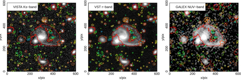
An example of this being applied to mismatching VISTA Ks-band (pixel scale 0.339 asec/pixEdge et al. 2013), Visual Survey Telescoper-band (VST; 0.2 asec/pixKuijken et al. 2015) and Galaxy Evolution Explorer NUV (GALEX; 1.5 asec/pixMartin et al. 2005) can be seen in Figure8. The remapping allows us to make a coordinate matched RGB colour image shown in Figure9, where the VISTA Ks-band and GALEX NUV-band data are remapped onto the WCS of the VST r-band data. The upsampling conserves flux, and by default uses bilinear interpolation (bicubic or nearest pixel, and forward or backward mapping, are also options).
[image:12.595.70.513.346.457.2]16 18 20 22
2
3
4
5
6
mag
R100/Kron−Radius
Stars
16 18 20 22
2
3
4
5
6
mag
R100/Kron−Radius
[image:13.595.42.273.108.422.2]Galaxies
Figure 6.The Kron to fully dilatedProFoundsemi-major axis (R100) expansion factor for simulated stars and galaxies.
23:29:14.0 23:29:12.0 23:29:10.0 23:29:08.0 23:29:06.0
−31:50:20
−31:49:40
−31:49:00
−31:48:20
Right Ascension / H:M:S
Declination / D:M:S
N E
Figure 7. Overlay of the intrinsic dilated segments (multi-coloured solid thin lines) and the inner Kron aperture (green el-lipses) and approximated elliptical apertures that best describe the dilated segment geometries (thick white dashed ellipses).
on the remapped target bands. Figure 10shows what this extraction might look like internally, where it is clear the majority of the GALEX NUV flux associated with the cen-tral spiral galaxy is enclosed by the VST r-band derived segments. Some of the fainter NUV features would be very hard to extract blindly, but should produce a reasonable signal when extracted in such a forced manner.
The above approaches are the best solution to extract-ing matched aperture total photometry. However, more ac-curate spectral energy distributions (SEDs) are often derived from using only the brighter inner parts of sources, since the outskirts usually include lowerS/N pixels which will act to increase the scatter between colours. Popular approaches to such colour photometry include fixed apertures (e.g. 2 asec circles placed on each source) or computing colours with a certain surface brightness level. The latter is achieved triv-ially inProFound, since one of the objects returned is the segmentation map before dilation, i.e. the segmentation that only includes pixels that are independently above some sur-face brightness threshold. An example of such a bright seg-mentation map is shown in Figure5, where the pixels iden-tified are much brighter than the fully dilated segmentation map shown in the right panel of Figure5. By using this map and turning off the option to dilate the segments high surface brightness colours can be extracted, leading to less scatter in the colour photometry measured (as we see in detail later using UltraVISTA data).
Finally, a hybrid colour is possible, where the bright seg-ment map is used as the starting point in each target image, but the segments are allowed to dilate independently in each target band in order to achieve converged flux. This is often similar in output to just applying the dilated segmentation map to each target band without allowing for independent dilation, however it can be a sensible option if the detection image has a much larger PSF than one or more of the tar-get bands, where the dilated aperture might be much larger than is actually necessary, and includes a large quantity of sky pixels which will lower the fidelity of the photometry extracted.
3 COMBININGProFoundWITHProFit
As discussed above, much of the design philosophy be-hind ProFound was to provide good quality inputs for
ProFitgalaxy profiling. This includes: careful sky subtrac-tion; sigma map construction via estimating the local sky-RMS map; good quality segmentation maps for extended sources and accurate initial conditions for the profile pa-rameters to use when fitting with theProFitengine.
Here we use these various elements of ProFound
to prepare the example VIKING data for a large multi-component fit5. Running ProFoundin default mode, but with the ‘boundstats’ option turned on, creates all the out-puts we need. In this example we aim to fit the central group of objects that have touching segments.
Figure11shows the main results, where the top panels show the initial parameter estimates taken fromProFound,
[image:13.595.46.273.476.714.2]0 100 200 300
0
100
200
300
x/pix
y/pix
VISTA Ks−band
0 200 400 600
0
200
400
600
x/pix
y/pix
VST r−band
0 20 40 60 80
0
20
40
60
80
x/pix
y/pix
[image:14.595.44.536.97.266.2]GALEX NUV−band
Figure 8.TheProFoundpackage comes with some highly WCS mismatched images of the same galaxy (GAMA galaxy ID G202627). The left panel shows VISTA Ks-band (pixel scale 0.339 asec/pix). The middle panel shows VSTr-band (0.2 asec/pix). The right panel shows GALEX NUV-band (1.5 asec/pix). Each image has dimensions of 2’×2’.
08:42:32.0 08:42:30.0 08:42:28.0 08:42:26.0
−00:17:00
−00:16:20
−00:15:40
Right Ascension / H:M:S
Declination / D:M:S
N E
Figure 9. RGB composite image of mismatching projections combing VISTA Ks-band, VSTr-band and GALEX NUV-band (as shown in Figure8) for the red / green / blue channels respec-tively.
and the bottom panels show the ProFitBFGS optimised solution. This particular fit uses S´ersic profiles for the two visually extended elliptical sources, and Moffat profiles for the remaining three objects which have PSF like character-istics. The Moffat PSF required for convolving the image and modelling the point-sources was estimated from fitting a number of isolated bright PSFs.
Overall we can achieve an excellent and rapidly con-verged simultaneous fit using this approach. The two ex-tremely bright stars in the bottom-right of the fit region have some residual structure, but the relative flux residu-als are generally small (a fraction of a percent). The other three sources are very well modelled, in particular the two
extended elliptical sources that have profiles very close to pure exponential discs.
The inputProFoundand outputProFitsource fluxes all agree within 0.4 mag, and the differences are typically less than 0.1 mag. Even the two close bright stars are well estimated by ProFound, with the differences being 0.07 mag fainter and 0.16 mag brighter. The total modelled flux in the fit region agrees to better than 1% with the extracted
ProFound flux. The Re for the S´ersic index is also well estimated, theProFoundinput increasing by∼5% for both of the clearly extended sources.
To achieve a rapidly converged fit for such complexes of objects the key requirements are that the objects are well segmented along flux saddle-points, and the initial es-timates for the fluxes and sizes are within a factor of∼2of the correct solution.ProFoundcan easily achieve these re-quirements if it is run in a sensible (usually near to default) manner. This suggests that usingProFoundcombined with
ProFitas part of an automated pipeline is a reasonable goal
for future large scale decomposition tasks.
4 SIMULATIONS
4.1 ProFitSimulations
To check the performance ofProFoundwe ran a number of tests using simulated data that was designed to approx-imately mimic the sky variations, sky RMS, PSF, magni-tudes, sizes and profiles of a mixture of stars and galaxies in a typical VIKING survey frame using the image genera-tion capabilities of ProFitto make the simulated frames. Table3details the various parameters and sampling ranges used when generating the simulated images. Code to repli-cate very similar types of simulations are also available on-line for user experimentation6. In order to ensure we have sources going much deeper than the noise threshold of the VIKING data, the selection of magnitudes, source sizes and
[image:14.595.45.274.328.561.2]0 200 400 600
0
200
400
600
x/pix
y/pix
VISTA Ks−band
0 200 400 600
0
200
400
600
x/pix
y/pix
VST r−band
0 200 400 600
0
200
400
600
x/pix
y/pix
[image:15.595.46.542.101.266.2]GALEX NUV−band
[image:15.595.84.239.370.571.2]Figure 10.Schematic view of theProFoundsegments defined using a common WCS system. In this case we use the WCS scheme from the VSTr-band image as seen in Figure8. The left panel shows the segments overlaid on the VISTA Ks-band. The middle panel shows the segments overlaid on the VSTr-band they were defined with. The right panel shows the segments overlaid on the GALEX NUV-band. Each image has dimensions of 2’×2’. It is notable that some of the GALEX NUV flux extends outside of the segment.ProFoundcan capture this additional flux if it is allowed to further dilate the provided segment (this is the default mode).
Table 3.The simulation setup parameters Simulation Parameter Value
N simulations 100
Sky 0
Sky RMS 10
magnitude zero point 30
x image pixels 1000
y image pixels 1000
PSF FWHM 5 pixels
N stars 200
Magnitude range 15–23 Magnitude Power-law slope 1.5
N galaxies 200
Magnitude range 15–23 Magnitude Power-law slope 2.0
Re Poissonλ 5
S´ersic index range 1–4 Axial-ratio range 0.3–1 Boxiness range -0.3–0.3
shapes was approximated using the deeper UltraVISTA sur-vey recovered usingProFound(see Section5). The PSF full width half max (FWHM) was chosen to be at the poorer ex-treme of values observed for VIKING:∼1.7 asec, or 5 pixels at the 0.339 asec/pixel scale of VIKING images (Edge et al. 2013).
Figure12is an example of the noise free model gener-ated byProFitfor the typical distribution of sources used for our simulations, the addition of noise and sky (estimated fromProFoundon real VIKING data) to create more real-istic looking data, and the extraction of sources using Pro-Found. In this example almost all of the stars were
success-fully recovered, and around half of the galaxies are detected, the rest being below the1σ surface brightness threshold of the VIKING survey.
ProFoundwas run with close to default settings, with
the difference being the de-blend tolerance (how many sky RMS deviations to use to de-blend sources during the
wa-tershed stage) was set to 1. These settings mimic the qual-itatively optimal settings we have determined for process-ing VIKING and UltraVISTA data withProFound(which in turn informed the majority of the default ProFound settings), but the broad results are quite robust to small changes in these settings.
One hundred 1k×1k frames were generated randomly withProFitmodel stars and galaxies and extracted with
ProFound, with 200 stars and 200 extended galaxies gener-ated per frame. This produces a final catalogue of 40k stars and galaxies generated. This is used to compute the false-positive and true-false-positive rates for stars and galaxies, and also quantify the measurement biases inProFound com-pared to the intrinsic sources. The latter is important since one of the main design aims ofProFound(along with better sky subtraction and flux converged segmentation maps) is to create reasonable initial conditions forProFitfits. These do not need to be perfect, but it helps to be reasonably close to the global maximum likelihood in order to speed up the fitting time. Based on our experience with the simulations presented inRobotham et al.(2017), a factor of two in flux and/or size is a reasonable starting point for efficient con-vergence (in detail this statement is clearly algorithm de-pendent, andProFitoffers no particular restriction on the optimization routine, giving out-the-box access to over 100).
Figure 13 shows the main completeness and spurious source extraction results forProFoundandSExtractor
ProFoundestimates for the model components
0 20 40 60 80 100 120
0
50
100
x/pix
y/pix
Data
0 20 40 60 80 100 120
0
50
100
x/pix
Model
0 20 40 60 80 100 120
0
50
100
x/pix
Data−Model
0 20 40 60 80 100 120
0
50
100
x/pix
χ=(Data−Model)σ
−50000
0
50000
−4
−2
0
2
4
−4 −2 0 2 4
0.01
0.1
χ
χ
norm(1)
Student−(2.1369)
−3 −2 −1 0 1 2
10
−
3
10
−
2
10
−
1
10
0
10
1
log10
(
χ2)
χ2
χ2(
1)
χν2=15.68
ProFitoptimised estimates for the model components
0 20 40 60 80 100 120
0
50
100
x/pix
y/pix
Data
0 20 40 60 80 100 120
0
50
100
x/pix
Model
0 20 40 60 80 100 120
0
50
100
x/pix
Data−Model
0 20 40 60 80 100 120
0
50
100
x/pix
χ=(Data−Model)σ
−50000
0
50000
−4
−2
0
2
4
−4 −2 0 2 4
0.01
0.1
χ
χ
norm(1)
Student−(4.0033)
−3 −2 −1 0 1 2
10
−
5
10
−
4
10
−
3
10
−
2
10
−
1
10
0
10
1
log10
(
χ2)
χ2
χ2(
1)
[image:16.595.82.501.100.759.2]χν2=2.03
Figure 12.Top-left is a real VISTA Z-band VIKING depth frame. Top-right panel shows the pure model created byProFitwith no noise added. Bottom-left panel adds realistic VIKING-like noise along with a variable sky background. The bottom-right panel shows the extractedProFoundsegments.
true-positive rate for the faintest sources when skycut∼0.8, after which point you almost certainly would not want to push the extraction much further since most of the addi-tional sources will be spurious. It should be noted that this limit is not trivially an extraction limit, since internal pixel smoothing and local clustering information is used to flag pixels that are likely to belong to real sources. Depending on the quality of the data and the pixel-to-pixel covariance the reasonable limit of skycut extraction might need to be higher than the value used here, however it is unlikely you could push much lower.
It is notable that the default extraction parameters of
SExtractorare a bit more conservative, extracting fewer
sources (and suffering the associated incompleteness) but with a lower false-positive rate. This comparison should not be considered exhaustive, since very different curves are pos-sible by changing the parameter setup of bothProFound