Liability Reduction through Demand Forecasting Improvement

(1)

LIABILITY REDUCTION

THROUGH

DEMAND FORECASTING IMPROVEMENT

Public version

Marleen Roerink

Master of Science in Industrial Engineering and Management

University supervisors: Company supervisor:

Dr. Ir. Petra Hoffmann Company X’ Data Analyst

(2)

(3)

COLOFON

Document: Master thesis

Title:

Liability reduction through demand forecasting improvement

Author:

M.H.W. Roerink

University:

University of Twente

Faculty:

Faculty of Behavioural, Management and Social Sciences

Programme:

Industrial Engineering and Management

Specialization:

Production and Logistic Management

Mailing Address: Postbus 217 7500 AE Enschede

Website:

www.utwente.nl

Graduation Date: May 2019

University Supervisors: Dr. Ir. Petra Hoffmann Dr. Engin Topan

(4)

(5)

Preface

Dear reader,

With pleasure I present to you my master thesis ‘Liability Reduction through Demand Forecasting

Improvement’. This report is the result of a research conducted at Company X in order to fulfil the graduation requirements for the study Industrial Engineering and Management with the specialization Production and Logistic Management at the University of Twente.

When I started my summer job at Company X in July 2018, I was impressed by the open culture and positive working atmosphere of the company. To get the chance to also execute my graduation project here from November 2018 on was delighting. I would like to thank employee A and employee B for granting me this opportunity. My special thanks go to employee B, who acted as my external supervisor, for his expertise and valuable input, which has been really helpful during the whole project. Furthermore, I would like to thank all colleagues from the Sourcing department for the great time. Being part of this team was a real pleasure.

Moreover, I would like to thank my supervisors Petra Hoffmann and Engin Topan. With the guidance of Petra in which direction to go, I found the right path to finish this thesis. Engin really helped me structuring the report, which has made it way better readable. Also, there was a certain time pressure, and thanks to their clear feedback and willingness to help me, I was able to graduate within the time frame that I had set myself the goal.

Furthermore, I would like to thank my university colleagues, without whom I wouldn’t have had such an

amazing time as a master’s student. In particular, I want to thank Nina and Suzan for making our exchange

to Taiwan unforgettable. This semester was definitely the highlight of my study period and it wouldn’t have

been without you.

Last, but certainly not least, I would like to thank my family and loved ones for their unconditional support.

All that remains for me is to wish you an enjoyable read.

(6)

(7)

Management Summary

Company X is a manufacturer of smart technical applications. In 2016, the company worked on a new strategic multi-year plan (Company X, 2018). With this plan, Company X wants to accelerate the organizational development by focusing on its core business, which is software development. As a part of this plan, their supply chain has been reorganized by outsourcing the production activities to strategic partners, so-called EMSs (Electronics Manufacturing Services).

The EMSs send a monthly file to Company X containing data about the inventory of components and materials they have in stock on behalf of Company X. Company X has deduced from these liability files that there is a lot of excess inventory, which is defined as the inventory that has no expected demand for one

year in advance. This excess inventory belongs to Company X’ liability, since they have agreed with the

EMSs to purchase it after there have been no call offs for twelve months. The Company X’ business units

that are included in the scope of this research are Business Unit A, Business Unit B and Business Unit C,

because the other business units have relatively less hardware.

The goal of this research is to improve Company X’ liability by reducing (and avoiding further creation of)

excess inventory at the EMSs.The main causes contributing to the buildup of this excess inventory are: high

Minimum Order Quantities (MOQs), demand forecasting errors, improper lifecycle management, and the leftover of the inventory buffer for the outsourcing process. An analysis after classification of the excess inventory to these causes using rules of thumb, showed that for Company X most excess inventory is assigned to the cause ‘forecasting errors’. These results in combination with the relatively high influenceability of this cause by Company X, has led to the focus of this research being the improvement of

Company X’ demand forecasting performance. The cause Lifecycle Management was ranked at the second

place, the cause High MOQs has given the lowest priority, and the cause ‘Leftover of the outsourcing buffer’

has been disregarded as core problem of this research.

In order to improve Company X’ forecasting performance, a literature review after forecasting methods

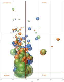
and different metrics for measuring the forecasting performance has been performed. What the most appropriate forecasting model for a certain product is, depends on its demand pattern. Demand patterns can be classified into four categories, based on two variables: the squared coefficient of variation (CV²), representing the variability in demand size, and the average inter-demand interval (ADI). A smooth demand pattern indicates that the product is well forecastable and a lumpy demand pattern implies a poor forecastability, which is defined as the ability to statistically forecast a product’s sales. The forecastability of the classes intermittent demand and erratic demand are in between, whereas intermittent demand has a relatively high ADI and erratic demand a relatively high CV².

Classification of Company X’ products to demand patterns showed that there are no significant differences

between the three business units. Most of Company X’ products have an intermittent demand pattern and

(8)

[image:8.612.76.326.73.396.2]

Figure 1: Bubble chart Company X’ demand patterns

An analysis on assessing the current forecasting performance of Company X indicates that the forecasts are neither stable nor accurate. The forecasting performance is divided in assessing the forecasting accuracy by calculating the Adjusted Mean Absolute Scaled Error (aMASE) and determining its bias by calculation of the course of the Mean Error (ME) over the year 2018.

For all business units, the value of the aMASE is higher than 1, implying that generating forecasts using the simple Naïve method would result in a smaller forecasting error compared to the current forecasting method. In the Naïve method the most recent observation is used as a forecast (Hyndman & Athanasopoulos, Forecasting: Principles and Practice, 2018). Hence, the values of the aMASE show us that there is certainly room for improvement of the demand forecasting accuracy of Company X.

(9)

stable. The negative outliers imply that there has been forecasted way too much, which results in excess inventories.

Demand forecasting at Company X is a decentralized process over the business units. We interviewed the employees who are responsible for these demand forecasting tasks in order to map the processes. All demand forecasting processes of the three different business units currently consist of many manual steps with judgmental input. This results in an inefficient and subjective forecasting process, since the forecasting task and its output are dependent of the person who executes it. This is not desirable in terms of flexibility and consistency.

We recommend applying statistical forecasting, in order to create less variability in the forecasted demand, to have a more efficient forecasting process and to have an increased forecasting accuracy by reducing the

subjectivity in the forecasting process. For intermittent demand, Croston’s method is the most frequently

used method, since it can deal with the zero values in the data (Doszyn, 2018). The basic idea of Croston’s

method is to divide the forecasted demand into two parts, which are both calculated using exponential smoothing; one for the size of the demand and one for the inter-demand interval (Croston, 1972). Nevertheless, also some limitations of Croston’s method have been addressed in literature, which have

given rise to adjustments to Croston’s method.

First, Syntetos, Boylan and Croston (2005) proposed to multiply the estimated demand with a certain factor in order to remove the bias that has been observed, resulting in the SBA method. This method has proven its performance for intermittent, erratic and lumpy demand patterns (Syntetos, Boylan, & Croston, 2005).

Second, the TSB method by Teunter, Syntetos and Babai (2011) tackles the issue of Croston’s method (and

the SBA method) that it does not adjust the forecast downwards in case of periods with zero demand. This issue is overcome by updating the demand probability instead of the demand interval, and doing so in every period. Finally, the Modified SBA method combines the adjustment of the SBA method in order to reduce the bias, with the idea of the TSB method to update the forecast also after periods of zero demand in order to deal with inventory obsolescence (Babai, Dallery, Boubaker, & Kalai, 2019).

Since both these adjustments are relevant for Company X and the Modified SBA method has shown positive results (Babai, Dallery, Boubaker, & Kalai, 2019), we recommend Company X to implement the Modified SBA method, whose formulas are shown below.

(10)

be reset by the employee(s) who is responsible for the forecasting task, by executing step 5 for each product again. The steps of the roadmap are:

• Step 1. Project initiation: define people, goals, tools and scope.

• Step 2. Product segmentation: select which products should be forecasted statistically, which ones

judgmentally and which ones should not be forecasted, based on their expected demand pattern.

• Step 3. Data exploration: analyze and preprocess the data. Perform a baseline measurement using

the forecasting performance metrics aMASE for accuracy and ME for bias (has already been done in this research). Perform time series decomposition on the demand data if there is a chance that it contains seasonality or a trend. An example of time series decomposition has been elaborated in appendix XIII. Split the time series data in a training set for model fitting and a test set for model testing (80-20 ratio).

• Step 4. Model selection: choose the statistical model(s). As explained before, we propose to apply

the modified SBA method. We recommend to also select a simple statistical forecasting method like the moving average method , in order to extent the framework of reference. Comparing the results of the Modified SBA method with both the zero measurement and the forecasting performance of a simple statistical method, provides insight in the results of applying statistical forecasting and the differences in forecasting performance of different statistical models.

• Step 5. Model fitting: estimate the model parameters. The modified SBA method contains

smoothing parameters (α and β), which require setting of their optimal values. This implies iteratively setting different values of these parameters and calculating the performance metrics over the training set. The combination of values which results in the lowest aMASE and ME close to zero is labeled as optimal. An example of model fitting has been elaborated in appendix XIII.

• Step 6. Model testing: calculate the aMASE (and ME) over the test set and compare. Generate

forecasts for the test set using each selected model (Modified SBA method and Moving average method). Calculate the aMASE and ME for these forecasts and compare these scores with the scores from the baseline measurement.

• Step 7. Process design: organize the forecasting task. The responsibilities concerning generating

forecasts, but also maintaining the forecasting model, must be assigned. Maintaining the forecasting model implies updating the dataset, controlling its performance by monitoring the forecasting errors and reviewing the statistical model. Review of the statistical model should be performed each year for each product, in order to re-establish the optimal values of the smoothing parameters. In case of non-stationary demand data, also the seasonal component and trend component should be updated by applying time series decomposition and model fitting, subsequently.

(11)

The recommended Modified SBA method deals with inventory obsolescence by adjusting the forecasted demand downwards after periods of zero demand. Notwithstanding, when a product reaches its end-of-life, this is not enough to avoid creation of excess inventory. Excess inventory due to the phasing-out of products should therefore be communicated proactively in a timely manner.

Furthermore, Company X should encourage its Product Development to use even more ‘shared

components’, especially for products which production is accommodated at the same EMSs. The benefits of more shared components are both the purchase price and the relatively lower MOQs. Additionally, the risk that inventory becomes obsolete decreases when its demand is divided over multiple products.

(12)

List of Tables and Figures

TABLE 1:INVENTORY OLDER THAN TWELVE MONTHS ... 18

TABLE 2:INVENTORY WITH ZERO DEMAND (INACTIVE AND OBSOLETE) ... 18

TABLE 3:EXCESS INVENTORY WITH SHELF LIFE ... 19

TABLE 4:COMPANY X SPECIFIC EXCESS INVENTORY ... 20

TABLE 5:EFFECT OF CONSOLIDATING DUPLICATE ROWS ... 21

TABLE 6:CLASSIFICATION MATRIX ... 23

TABLE 7:ASSESSMENT MATRIX... 28

TABLE 8:DECISION MATRIX ... 28

TABLE 9:FORECASTING ROWS COMPANY X ... 53

TABLE 10:COMPARISON OF FORECASTING PROCESS ... 54

FIGURE 1:BUBBLE CHART COMPANY X’ DEMAND PATTERNS ... VIII FIGURE 2:PROFIT OF COMPANY X FROM 2014 TO 2017 ... 1

FIGURE 3:SUPPLY CHAIN ... 2

FIGURE 4:PROBLEM CLUSTER ... 10

FIGURE 5:EMSS RELATED TO COMPANY X’ DEMAND ... 14

FIGURE 6:VISUALIZATION OF COMPANY X’ FINANCIAL RISK REGARDING INVENTORY ... 16

FIGURE 7:EXCESS INVENTORY CLASSIFICATION ... 17

FIGURE 8:PART OF SPEND THAT HAS A SHELF LIFE ... 19

FIGURE 9:PART OF SPEND THAT IS COMPANY X SPECIFIC ... 20

FIGURE 10:CHART EXCESS INVENTORY CLASSIFICATION TOTAL ... 25

FIGURE 11:GRAPH EXCESS INVENTORY CLASSIFICATION PER MONTH... 25

FIGURE 12:GRAPHS TOTAL EXCESS INVENTORY PER EMS AND PER BUSINESS UNIT ... 26

FIGURE 13:DEMAND PATTERNS ... 35

FIGURE 14:FRAMEWORK FOR FORECASTING (SILVER,PYKE,&THOMAS,2017, P.74) ... 37

FIGURE 15:FORECASTING PROCESS CYCLE (DUFFUAA &RAOUF,2015, P.21) ... 38

FIGURE 16:DIVIDING TIME SERIES IN DATA SETS ... 39

FIGURE 17:MULTIPLICATIVE DECOMPOSITION OF AIRLINE PASSENGER DATASET ... 46

FIGURE 18:SBC CLASSIFICATION MATRIX (SYNTETOS ET AL.,2005) ... 49

FIGURE 19:CROSS VALIDATION ... 50

FIGURE 20:CLASSIFICATION OF DEMAND PATTERNS ... 56

FIGURE 21:DEMAND PATTERNS BUBBLE CHART... 57

FIGURE 22:DELIVERY PERFORMANCE EMSS ... 60

FIGURE 23:SCORES AMASE ZERO-MEASUREMENT ... 60

FIGURE 24:BIAS BUSINESS UNIT B ... 61

FIGURE 25:BIAS BUSINESS UNIT C ... FOUT!BLADWIJZER NIET GEDEFINIEERD. FIGURE 26:BIAS BUSINESS UNIT A ... 62

(16)

List of Abbreviations

Abbreviation Definition

ADI Average inter-Demand Interval

AIC Akaike's Information Criterion

ANOVA Analysis Of Variance

BIC Bayesian Information Criterion

BU Business Unit

CC Computational Complexity

CM Croston's Method

CoV/CV Coefficient of Variation

CRM Customer Relationship Management

EMS Electronics Manufacturing Service

EOL End Of Life

EOQ Economic Order Quantity

ES Exponential Smoothing

FC Forecast

GMAE Geometric Mean Absolute Error

GMRAE Geometric Mean Relative Absolute Error

IOS Inactive, Obsolete, Surplus

LLI Long Leadtime Item

MAD Mean Absolute Deviation

MAE Mean Absolute Error

(s)MAPE (Symmetric) Mean Absolute Percentage Error

MASE Mean Absolute Scaled Error

MdRAE Median Relative Absolute Error

ME Mean Error

MOQ Minimum Order Quantity

MPE Mean Percentage Error

MRO Maintenance, Repair and Operating

(R)MSE (Root) Mean Squared Error

MTO Make To Order

MTS Make To Stock

PCB Printed Circuit Board

Production Facility X Company X’ production facility

RCA Root Cause Analysis

SEATS Seasonal Extraction in ARIMA Time Series

SKU Stock Keeping Unit

SLA Service Level Agreement

VBA Visual Basic for Applications

(17)

Introduction

This Master thesis project is performed on behalf of Company X. In section 1.1, Company X as a company is introduced. Section 0 provides some background information about the research assignment at Company X. Section 1.3 presents information from literature about the concerned topics. In section 1.4, the problem is discussed. This is followed by an explanation of the research design and the scope of the research in section 1.5 and 1.6, respectively.

1.1. Company X

Company X consists of multiple business units, since different problems require a different field of expertise. Each one of these business units has deep insight into their particular market, resulting in innovative technological systems that focus on relevant issues for now and in the future. The Company X business units and their core products are:

- Business Unit A: loss prevention and stock management systems.

- Business Unit B: systems for monitoring and caring using individual animal identification.

- Business Unit C: light management systems for the industry.

- Enumeration of the other business units

Together, these Company X’ business units account for

approximately XX million euros of profit (excluding one-off items, which are expenses or revenues from non-recurring

activities, so outside a company’s usual business

operations), see Figure 2.

Since its founding, Company X has been manufacturing smart technical applications. In 2016, the company worked on a new strategic multi-year plan (Company X, 2018). With this plan, Company X wants to focus on accelerating the organizational development by focusing on its core business, which is software development. For example, their product range will be reduced from approximately 1000 to 400 technological solutions. These products can consist of only software or a combination of both software and hardware.

As another part of this plan, their supply chain is reorganized by outsourcing the production activities to

strategic partners and closing Company X’ production location. To manage this process the department

Sourcing, which overarches the business units, was brought into being.

(18)

1.2. Research motivation

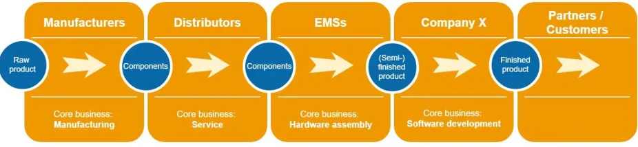
The research assignment is performed on behalf of the Sourcing department. Company X has outsourced its production activities to so-called Electronics Manufacturing Services, hereafter called EMSs. In the contracts with the EMSs, Company X agreed on an open cost price calculation model. Hereby, Company X has insight in the prices the EMSs pay for the different components. The general supply chain of the

[image:18.612.75.538.172.279.2]

products of all Company X’ business units is visualized in Figure 3: Supply chain.

Figure 3: Supply chain

Company X has contracts with about six EMSs. This number is dynamic, since some projects are shifted from one EMS to another. Per project, which is one or a bundle of Company X products, Company X has Service Level Agreements with the EMS. The Company X business units specify which manufacturer supplies which component of the product they are developing. The Sourcing department of Company X selects in consultation with the concerned Business Unit the EMS per project. Most manufacturers sell their components through distributors and not directly to EMSs. Therefore, the EMS can select their own suppliers (distributors), as long as they purchase the components from the manufacturer specified by the Company X Business Units.

Some components are fabricated based on Company X specifications, further referred to as ‘Company X

specific components’. These components are directly distributed from the manufacturer to the EMS. Generally, the manufacturers require high Minimum Order Quantities (MOQs) on these components, which might results in excessive inventory levels.

Each EMS is responsible for managing their own inventory of components and materials for Company X. The Company X Business Units send weekly forecasts with their expected demand for one year in advance to the EMSs. The EMSs produce to Company X orders, but have to manage their inventories of components

based on these demand forecasts of Company X. The four biggest EMSs, based on the value of Company X’

demand, provide monthly data of their inventory in a so-called liability overview.

The Sourcing department of Company X has deduced from these data that the EMSs have a lot of excess inventory. This poses a financial risk for both the EMSs and Company X. The financial risk for Company X regarding the excess inventory at the EMSs and its causes are explained in more detail in the problem description in section 1.4. The size of the problem is indicated by quantifying the financial risk for Company

X in section 0. We define ‘financial risk’ as any measurable risk that can have financial consequences.‘Excess

inventory’ is the part of the inventory of components for which no Company X demand (order or forecast)

is known. The goal of this research is to improve Company X’ liability by reducing the excess inventory of

(19)

Company X’ liability concerning the excess inventory at the EMSs constitutes a discrepancy between the norm and reality for Company X. Hence, we can conclude that the problem of Company X regarding the excess inventory is an action problem, according to the definition of Heerkens and Van Winden (2012). The Management Problem Solving Method (MPSM) is a framework for solving an action problem (Heerkens & Van Winden, 2012). This method consists of seven phases, which are elaborated in the chapters and sections mentioned per phase:

1. Problem identification: section 1.4 Problem identification

2. Solution planning: section 1.5 Research design

3. Problem analysis: chapter 2 Problem analysis

4. Solution generation: chapter 3 Literature review

5. Solution choice: chapter 5 Improvements

6. Solution implementation: chapter 5 Improvements

7. Solution evaluation: chapter 5 Improvements

(20)

1.3. Theoretical background

In this section the background information about excess inventory and its causes according to literature is

explained. In order to better understand what kind of inventory Company X’ problem is about, the relevant

theory behind inventory classification is described in section 1.3.1. Also the definitions of different kinds of inventory and especially of excess inventory are discussed in this section. To clarify what inventories exactly belong to the excess, approaches for determining the excess inventory levels are explained in the section 1.3.2. Subsequently, the possible causes of excess inventory according to literature are explained in section 1.3.3. This theory serves as input for the problem cluster.

1.3.1. Inventory classification and definition

Generally, inventory can be classified in two types based on whether it effectively serves a function or not. The inventory that does not effectively serve a function is excess.

“Inventory is a current asset that should more than earn its keep; if inventory incurs more costs than

benefits, it is really a liability. Excess inventory is clearly an operational liability.” (Toelle & Tersine, 1989).

In literature, excess inventory is defined in several ways. Nnamdi (2018) defines excess inventories as the Stock Keeping Units (SKU’s) that have a significant amount of inventories on-hand compared to average annual consumption. Crandall and Crandall (2003) state that “in essence, inventory is not excess when it is in the right quantity of the right goods at the right place at the right time”. As stated by Rosenfield (1989) is inventory excess when “the potential value of excess stock, less the expected storage costs, fails to match the salvage value”. According to Toelle and Tersine (1989), excess inventory is any item that not effectively serves one of the following functions:

- Working stock (cycle or lot size stock). Inventory that is held so that ordering and production can

be done using an economical lot size instead of on an as-needed basis.

- Safety stock (buffer or fluctuation stock). A buffer of inventory which protects against the

consequences of uncertainties in supply and demand.

- Anticipation stock (seasonal or stabilization stock). Inventory which is held to deal with peak seasonal demand and unusual requirements as strikes or vacations.

- Pipeline stock (transit or work-in-process stock). Inventory that is being processed or transported

within or between facilities.

- Decoupling stock. Inventory within a production or distribution process so that one stage of the

process does not slow down other parts of the process.

These definitions of excess inventory have all in common that inventory belongs to the excess, when it will not be used within a certain timeframe and can therefore be labelled as inefficient.

(21)

- Materials/components. This type of inventory includes all materials/components to be used as input in the manufacturing process.

- Work-In-Progress. This includes the inventory of any unfinished goods (semi-finished goods) that

have been made by the company.

- Finished goods. This type of inventory includes any finished goods produced that are ready for sale.

As will be motivated in section 1.6, this research is scoped to the inventory type ‘materials/components’

only. In turn, the excess inventory of this type can be categorized in different types. Toelle and Tersine (1989) distinguish three operational types of excess inventory:

- Dead stock. This is the inventory which has not been used for a specific length of time, so the inventory that does not turn over (anymore).

- Degraded stock. This stock consists of items which do not meet the quality requirements (any

longer). These items can for example be spoiled, damaged or deteriorated.

- Slow-moving stock. These are the items of stock on hand which retain their full utility and which

have a continuing demand, but which have a higher amount on stock than can be justified by the anticipated rate of future demand (Toelle & Tersine, 1989).

A different classification of excess inventory is made by Bragg (2011). He states that IOS inventory (Inactive, Obsolete, Surplus) consists of the following parts:

- Inactive. These are the parts on stock that have no forecasted usage.

- Obsolete. These parts are no longer incorporated in any current product.

- Surplus. The inventory levels of these parts exceed the forecasted usage.

In section 2.2.1 we use the definitions of these two different classifications for determining what belongs to the excess inventory according to Company X.

1.3.2. Determination of excess inventory levels

There are also multiple ways of determining the excess inventory levels. From simple models in which time value corrections are ignored to more complicated models which consider the inflations and time values through a present value correction (Tersine & Toelle, 1984). The method of determining the excess inventory levels also depends on the used definition of excess inventory and which corresponding operational types are taken into account. For determination of the excess inventory levels of slow-moving-items Toelle and Tersine (1989) state three possible approaches, which are explained in the following paragraphs.

One approach is to set a certain time supply as the tolerable time supply of stock on hand. A 12-months’

supply is often used as a benchmark, because inventory that will not be used within this time interval is not really a “current asset” (Toelle & Tersine, 1989).

Another approach of determining the excess inventory levels is to refer to previously established inventory policies, like the EOQ. In that case, the excess inventory is defined as the difference between the actual inventory levels and the sum of the lot size and safety stock (Toelle & Tersine, 1989). In case of inventory control by using for example a min-max system, every item that exceeds the maximum inventory level belongs to the excess inventory. When a company has the objective to have at least four inventory turns

per year, the (potential) excess inventory would consist of every item that is not needed for a three-months’

(22)

In the third approach mentioned by Toelle and Tersine (1989) the excess inventory is determined by calculating for what part of the inventory the liquidation would be economically justifiable. This approach defines what part of the slow-moving items should be liquidated in order to minimize relevant costs. Herewith this decision-oriented approach serves as a guide to action once the excess inventory levels have been established (Toelle & Tersine, 1989).

1.3.3. Causes of excess inventory

There are numerous reasons for a surplus or obsolete inventory mentioned in literature. No author states to have an exhaustive list of possible causes of excess inventory, because these causes differ from organization, industry, situation, and so on. The reasons may vary from (Tersine & Toelle, 1984): a change in methods of production, new technological innovations to an over-zealous purchasing practice. Some examples of potential causes mentioned by Willoughby (n.d.) are: price increases, customer cancellations, the introduction of a new (competing) product or changing business conditions.

A distinction in the possible causes can be made based on the kind of inventory. For example, a part of the possible causes are particularly for the excess inventory of spare parts, like a change in maintenance policy or the use of alternative spare parts. Some frequent general causes of excess inventory stated by Toelle and Tersine (1989) are:

o Forecasting errors. Negative differences between the predicted and actual demand and the failure

to anticipate on it usually result in excess inventory levels.

o Inventory record inaccuracies. Errors in for example disbursements, stock levels, part identification

numbers, etc. often manifest in excess inventory.

o Inadequate planning and execution systems. The use of decent planning methods, correct and

accurate purchase or work orders, and an adequate production scheduling and control system are part of the basis for proper inventory control.

o Long or variable lead times. Long production times result in a build-up of work-in-process stock and

variable production lead times generally ask for higher safety stocks.

o Obsolescence. Whenever a product reaches its end-of-life, the demand will drop down. Engineering

change activities such as product redesign or product termination should therefore be planned and coordinated very well.

o Master schedule smoothing. The planned rate of supply may not exactly match the (expected) rate

of demand in order to achieve manufacturing efficiencies, which can cause an accumulation of stocks.

o Distribution channel adjustments. When stocking and shipping policies change within a distribution

channel, it can appear to the source as real increases in customer demand. If the production activities of the source are increased in response to this, excess inventory arises.

o Changes in inventory holding costs. A sudden increase in inventory holding costs can make

inventory reductions imperative. Although the number of units which are physically on stock remain the same, the accepted inventory levels might change, which causes an excess of inventory.

(23)

o Demand variation. Product proliferation and shorter product cycles contribute to more uncertainty in the demand, which makes it harder to make an accurate demand forecast. When a company does not properly track the life-cycle stages of a product, an excess inventory is a possible consequence. Not only the product cycles, but also economic cycles contribute to the forecasting problem, since it seems that companies fail to act proactively to an economic slowdown or upturn.

In addition to that, the demand variability increases as one moves up the supply chain (Chen, Drezner, Ryan, & Simchi-Levi, 2000). This phenomenon in supply chain management is known as the bullwhip effect. The five main causes of this effect are: the use of demand forecasting, supply shortages, lead times, order batching, and price fluctuations (Chen, Drezner, Ryan, & Simchi-Levi, 2000). More information about this phenomenon is provided in section 3.3.

o Supply variation. Excess inventory can arise when for example a supplier does not have sufficient

capacity or no consistency in their delivery times. Also volume discounts can be a trigger to purchase more than needed.

o Internal variation:

▪ Sales and Marketing: they sometimes want to have excess inventory available for

a fast response to customer demand.

▪ Engineering: when the product design is improved, engineers are mostly impatient

to see the effect. New product designs require additional inventories and cause that existing inventories become obsolete.

▪ Production Planning and Purchasing: to avoid fluctuations in the workforce,

production planners prefer producing at a balanced workload. In combination with a fluctuating demand, this can cause an excess in the finished goods inventory.

▪ Accounting/Finance: sometimes it seems to be attractive to buildup inventory,

(24)

1.4. Problem identification

The problem assignment provided by Company X is that their liability is too high, due to excess inventory at the EMSs. Several causes contribute to this problem. The first phase of the MPSM concerns the problem identification resulting in a problem statement (Heerkens & Van Winden, 2012). We elaborate this phase of the MPSM in this section.

The consequences of the excess inventory are explained in section 1.4.1, followed by an explanation of its causes in section 1.4.2. Both the consequences and causes have been assigned to a color, which refers to the color of these blocks in the problem cluster. The causes have been identified by having conversations with Company X employees and using the information about possible causes according to literature. Finally, in section 1.4.3 the causes and consequences are schematically presented in a problem cluster and the core problem is explained.

1.4.1. Consequences

Each month the biggest EMSs of Company X send an overview of the actual inventory they have on behalf of Company X, so Company X is proactively informed about (potential) excess inventory. The inventory

consists of components that the EMSs need for manufacturing of Company X’ products. Most of this

inventory is allocated to a certain demand, which is a Company X order or a demand forecast provided by Company X. For the remaining part of the inventory there is no demand. This is what Company X and the EMS call ‘excess inventory’.

Aging of components: This excess of inventory poses a financial risk, since when Company X does not expect to have any demand for a certain component in the future, this component becomes waste to Company X. Moreover, some components have a certain shelf life, so are perishable. In some cases, it is worth the effort to sell such inventory. Nevertheless, the value of the components deceases by time, which implies that they will never yield the same as they have cost. Therefore, there is always a financial loss on aged components that will not be used by Company X anymore.

Company X specific components: There are also components that can never be sold, since they are

fabricated based on Company X’ specifications. No other company uses them. Hence, this is waste

of material and therefore a financial loss.

Contracts: Company X has agreed with their EMSs that they will repurchase the inventory after it has not been used in twelve months. Therefore Company X foots the bill of the financial risk that goes along with the excess inventory.

1.4.2. Causes

According to the theoretical background in section 1.3.3., there are several possible causes of excess

inventory. Some of these causes are only relevant for excess inventory in finished goods, like ‘insufficient

production capacity’. Since this research is scoped to inventory of materials and components, these

possible causes are eliminated. Other possible causes according to literature simply do not apply to the situation of Company X, like handling financial performance measures that make buildup of inventory attractive.

(25)

outsourcing process. After the outsourcing process, there was still a big part of this buffer left, so Company X requested their EMSs to take over this inventory from Production Facility X. Therefore, some of the current excess inventory at the EMSs could be leftovers from the inventory buffer of Production Facility X.

Lack of incentives to purchase efficiently: Company X has contractually agreed that the EMSs are allowed to purchase based on Company X forecast, Minimum Order Quantities (MOQs) and lead times of components. However, these agreements have not always been defined quantitatively. Also, the consequences of excessive inventory levels at the EMSs are mostly the risk of Company X, since Company X has to repurchase it after twelve months. These agreements result in that currently the EMSs have no additional incentives to optimize their inventory levels, except for the holding costs and the physical space they have available. According to literature, also wrong performance measures can result in the EMSs holding too much inventory.

Unreliable and long lead times: The EMSs can have several reasons to order more than the demand

is. For some components, the lead time is long and unreliable due to the current market’s scarcity.

Therefore, the EMSs order more than needed to ensure the order fulfilment and therewith create a buffer of components.

Inventory record inaccuracies: Errors in actual inventory levels might result in unnecessary purchase orders of components. This in turn results in excess inventories.

High MOQs: Another cause for higher order quantities of the EMS than needed to fulfil Company

X’ demand, is the MOQs of the EMSs’ suppliers. Generally, a higher MOQ results in a lower price

per component and the other way around. Also, a part of the components in the Company X products are fabricated based on Company X’ specifications, the so-called ‘Company X specific components’. This implies that these components are not generic and therefore the manufacturer requires high MOQs. The MOQs are a problem to the EMSs of Company X, because Company X has products with mostly high variety and low volumes. This might causes that the MOQs of the suppliers of the EMS are too high for the demand of Company X.

Demand forecasting errors of Company X: Every week, the EMSs receive a demand forecast of the Company X business units. Generally, they forecast one year in advance but some of the business units might deviate from this. Each business unit forecasts on their own manner. There might be some uniformity in the forecasting formats of some business units, but the expected demand levels are determined in different ways. Also, the Sales department of the business units do not have an incentive to provide accurate demand information, since they will not be called to account for the accuracy of their forecast information. The interests of Sales are in general not totally similar to the interests of Operations, because Sales focuses more on delivery performance instead of efficiency. Therefore, their sales forecasts are often too high, which results in an excess inventory at the EMSs.

(26)

1.4.3. Problem cluster

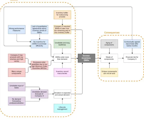
[image:26.612.74.551.146.539.2]

The problem cluster is a method for structuring the problem context by mapping the different problems and their interrelationships (Heerkens & Van Winden, 2012). The problem of Company X concerning the inventory at the EMSs is schematically represented in Figure 4.

Figure 4: Problem Cluster

Heerkens and Van Winden (2012) state that the core problem must be influenceable, has no other causes and is the problem which has the greatest effect in case of multiple problems (Heerkens & Van Winden, 2012).

The causes that qualify for being the core problem of this research are selected from the problem cluster.

Causes that are not really influenceable by Company X are therefore omitted. Hence, the cause ‘Unreliable

and long lead times’ is eliminated. Also the cause ‘Remainder inventory buffer from Production Facility X’

is not influenceable anymore, since this was a one-time event from the past. The cause ‘inventory record

(27)

structural quality and logistic audits at the EMSs. Since inventory management belongs to the responsibility

of the EMSs, the cause ‘inventory record inaccuracies’ does not qualify for being the core problem.

There are multiple remaining causes that qualify for being the core problem. These causes are:

o High MOQs. The MOQs are too high for Company X’ demand, this is partly caused by using many

Company X specific components, which have generally higher MOQs compared to generic components.

o Lack of incentives to purchase efficiently. Due to the lack of qualitative agreements, for example

about allowed inventory levels, or due to wrong performance measures, for example delivery performance, the EMSs are not triggered to optimize their inventory levels.

o Demand forecasting errors of Company X. A lower actual demand compared to what was forecasted

results in an excess inventory of components that already have been ordered to fulfil the forecasted demand.

o Lifecycle management: No proper keeping track and communication about the life-cycle stages of

a product might result in excess inventories when a product is phased out.

To be able to determine and motivate what the core problem of the excess inventory is, more research after the causes and their effect on the inventory levels is required. Hence, we first have a knowledge problem we have to solve, before we can continue with solving the action problem regarding the excess inventory.

The analysis after identification of the core problem is elaborated in chapter 2. The problem statement of the knowledge problem is: A lack of insight in the causes of the excess inventory to be able to identify the core problem of this research. This leaves us with a rather general problem statement for the action

(28)

1.5. Research design (knowledge problem)

The problem where the Sourcing department of Company X took note of is described in the previous section. We explained in section 1.4.3 that we first have to solve a knowledge problem, namely identifying the core problem of excess inventory at the EMSs. This section presents the research plan for solving this knowledge problem. Herewith we elaborate phase 2 of the MPSM: solution planning (Heerkens & Van Winden, 2012).

The procedure of solving a knowledge problem is the research cycle, which consists of eight phases (Heerkens & Van Winden, 2012):

1. Research aim

2. Problem statement

3. Research questions

4. Research design

5. Operationalization

6. Measuring

7. Analysis

8. Conclusions

The research aim of this knowledge problem is to identify the core problem and the problem statement is the lack of insight in the causes of excess inventory at the EMSs that qualify for being the core problem.

Phase 3 and 4 are included in this section. In section 0 and 2.3, both phase 5 and 6 are elaborated in by quantifying the size of the problem and the extent to which the causes contribute to the problem. In section 2.4 the results of this classification are analysed, by which phase 7 is completed. Finally, in section 2.5 we draw some conclusions about the identification of the core problem. Herewith we execute phase 8 of the research cycle and provide the answer the knowledge problem.

To be able to solve the knowledge problem, the following sub questions will be answered by the approach mentioned per question.

RQ: What is the core problem regarding excess inventory at the EMSs for Company X?

The research question will be answered by first determining the size of the problem in sub question 1 and thereafter prioritizing the causes in sub question 2.

SQ1: How big is the financial risk for Company X that goes along with the excess inventory?

This sub question is answered in section 0. The answer to this sub question provides an indication of the size of the problem for Company X. First, by analysing what Company X and the EMSs have agreed about the inventory levels and the corresponding responsibilities, the link between the excess inventory and why this poses a financial risk for Company X is clarified in section 2.1. The contractual agreements between Company X and the EMSs are examined for determining what part of the inventory at the EMSs belongs to the liability of Company X. In section 0, the consequences described in the problem cluster are quantified by analysing the liability files which are sent by the EMSs to Company X monthly.

(29)

This sub question is already partly answered by the problem cluster in section 1.4.3, because the problem cluster shows the possible causes of excess inventory. In section 2.3 the causes derived from the problem cluster that qualify for being the core problem are further analysed.

Quantification of these causes is required for determining how much a certain cause contributes to the problem. For this, the liability files of the different EMS are analysed. The liability files contain data that the EMSs derive from their ERP-system. This is the only information available for Company X regarding their liability due to excess inventories at the EMSs. The excess inventory is classified per cause by assigning the excess inventory per component to a certain cause. This classification is based on rules of thumb, since the data consists of too many rows (different components) to analyse them one by one. As a result of this analysis, the causes are given a priority in section 2.4.

(30)

1.6. Scope

Company X and the EMSs define excess inventory as the inventory on stock and on order for which no demand (order or forecast) is known, because this inventory actually poses a financial risk to Company X. This inventory can consist of finished goods, as well as it can consist of components and materials. The finished goods are out of the scope of this research, since this inventory is not stored at the EMSs and is therefore not included in the liability files, from which Company X derived that there is too much excess inventory. Moreover, excess inventory of finished goods might require a different approach since it is

possibly caused by a different core problem. Hence, this research is scoped to the EMSs’ excess inventory

of ‘components and materials’ (hereafter referred to as components) on behalf of Company X.

Figure 5 shows which EMS accounts for which part of the annual demand of Company X. The demand of Company X for 2018 is based on the known figures of the first half year of 2018 and an estimation of the figures for the second half year of 2018.

Figure 5: EMSs related to Company X’ demand

The three biggest EMSs account together for 82% of Company X’ demand in 2017 and for 81% of Company

X’ demand in 2018. The remaining three EMSs are currently in a transition to producing a bigger or smaller

part of Company X’ demand, so they have limited historic data about inventories for Company X. Therefore,

this research is scoped to the three biggest EMSs of Company X, which are EMS 1, EMS 2 and EMS 3.

Company X still has an own production facility, called Production Facility X, in which some of the Company X products are produced or assembled. Some of the EMSs are suppliers of Production Facility X, so Production Facility X can be considered as both a Company X Business Unit and a supplier. Because of this, there could be some overlap in the inventory data of Production Facility X and the EMS. Since we cannot ensure the reliability of the data, Production Facility X is not considered as one of the EMSs, so left out of scope of this research.

(31)

Problem analysis

This chapter contains the problem analysis concerning the excess inventory at the EMSs and provides the answer to the knowledge problem. Hereby, phase 3 of the MPSM of Heerkens and Van Winden (2012) has been carried out.

Section 2.1 describes what Company X contractually agreed about allowed inventory levels of components and the performance measures they will assess the EMSs on. Section 0 provides an indication of the size of the problem for Company X regarding the excess inventory by quantification of the financial risk. Subsequently, section 2.3 contains an analysis to determine which causes contribute most to the excess inventory. This analysis is based on classifying the excess inventory from the liability files that the EMSs sent to Company X monthly. In section 2.4 the identified causes are prioritized. Herewith the research question of the knowledge problem is answered. Based on this, the research design for the action problem has been drawn up in section 2.6.

2.1. Contractual agreements

The problem cluster shows that the contractual agreements between Company X and the EMSs are both a cause of excess inventories and a reason the excess inventories pose a financial risk to Company X.

Company X has purchase agreements with each one of the EMSs. In addition to these agreements, per project (a bundle of Company X products) additional SLAs are drawn up. These SLAs have different themes, for example Quality, Tooling or Logistics. Both the SLA Logistics and Purchase Agreement are relevant for this research, since they contain agreements regarding the purchasing of components and the allowed inventory levels. We derived the information which is relevant for this research from these contracts. These agreements are listed in appendix I.

The qualitative agreements from the purchase agreements and SLAs between Company X and the EMSs are mostly similar over the EMSs. Only the quantitative agreements in the Logistic SLAs are rather different since they concern a specific project. Company X has agreed with the EMSs that the following parameters will be set per product and should be reviewed every 6 months:

- Purchase price per product per piece;

- Production batch size;

- Production lead time;

- Single package quantity;

- Safety stock for components;

- Safety stock for semi-finished products;

- Safety stock for finished products.

(32)

currently the financial risk of Company X is according to the contracts. Figure 6 visualizes the inventory of the EMSs and the financial risk of Company X regarding this inventory.

[image:32.612.88.540.187.461.2]

Company X has agreed to purchase the inventory of the EMSs after there have been no call offs after one year, see agreement eleven of appendix I. All inventory that has no demand is either already they liability of Company X or poses the risk to become the liability of Company X in the near future. Therefore, we include all inventory that is excess for determination of the financial risk of Company X. In Figure 6 this part of the inventory is represented by ‘has no demand, so is excess’.

Figure 6: Visualization of Company X’ financial risk regarding inventory

The proportions of the inventory in Figure 6 are not representative. Hence, Figure 6 only shows how the inventories can be broken up, but not in which proportions they are related.

The Key Performance Indicators (KPIs) where Company X and the EMSs contractually agreed upon regard only the logistical performance of the EMSs. These agreements are included in appendix I. Since only logistical KPIs have been defined, it seems that the EMSs are strictly assessed on their delivery performance. However, how these performance measures are defined indicate that this is not the case. Only target levels have been defined and no consequences are associated with non-performance. After inquire at the logistics auditor of Company X, we can conclude that the EMSs are assessed mildly on their delivery performance. He also states that the EMS desire to have low inventory levels as well. In the end, they foot the bill for the holding costs regarding these excess inventories. Hence, we eliminate ‘lack of incentives to purchase

(33)

2.2. Quantification of financial risk for Company X

In this section, the size of the problem is indicated by quantifying its consequences. This analysis is performed in order to determine whether the problem is actually worth investigating. As shown in the problem cluster of Figure 4, the excess inventories at the EMSs result in a financial risk. First we agree about what part of the inventory can be considered as excess inventory in section 2.2.1. In the subsequent sections, we quantify the main consequences of excess inventory, namely repurchasing and waste, respectively.

2.2.1. Excess inventory determination

Company X’ definition of excess inventory is: inventory on stock and on order that has no demand (order

or forecast). The demarcation of excess inventory according to literature is broader than what belongs to

excess inventory in Company X’ perception. See section 1.3.1 for what is stated in literature about defining

excess inventory.

Obviously, the categories ‘deadstock’, ‘degraded stock’, ‘obsolete’, and ‘inactive’ are also excess inventory

according to Company X’ definition. This is less clear for the category ‘slow-moving stock’, because this

includes the inventory which does have enough demand, but which is inefficient to have on stock already (the stock cannot be justified by the anticipated rate of future demand). Since this part of the inventory

does not directly pose a financial risk to Company X, we decided to exclude it from our definition of ‘excess

inventory’.

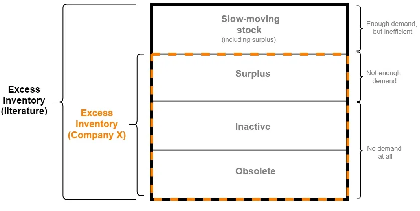
[image:33.612.84.505.433.645.2]

The inventory that is considered as excess inventory in this research is therefore a part of the inventory that is excess according to literature. The scope of excess inventory that is maintained in this research is shown in figure 7.

Figure 7: Excess inventory classification

Every item on stock or on order (future stock) which cannot be assigned to a certain demand is excess inventory. Therefore, the formula for determining the excess inventory levels is:

(34)

2.2.2. Repurchase

Company X has agreed with their EMSs that if there has been no call off within one year for certain

inventory, Company X will purchase it from the EMSs. The column ‘financial risk’ in Table 1 shows the total

value of the excess inventory that had no call offs for twelve months or longer at the three biggest EMSs of Company X. This analysis is performed in November 2018 with actual data, so all excess inventory with a

last-usage date in the 3rd_{quartile of 2017 or earlier is included.}_{The column ‘Near future risk’ shows the}

part of the excess inventory which has a last-usage date in the 4th_{quartile of 2017, so which poses a financial}

risk in the near future.

Table 1: Inventory older than twelve months

EMS 2 does not provide information about the value in combination with the age of the inventory. The

current financial risk due to the agreement of takeover of the inventory is therefore at least €XX. Moreover,

the excess inventory covers XX% of the total inventory.

Some components from this excess inventory have no demand at all. Figure 7 classifies this inventory as ‘inactive’ or ‘obsolete’. The total value of the excess inventory with zero demand is for the three EMSs €XX, which accounts for XX% of their total excess inventory. Table 2 shows the distribution of this excess inventory over the EMSs. EMS 2 has zero excess inventory that has no demand at all, since they produce the Company X products with a continuing demand.

Table 2: Inventory with zero demand (inactive and obsolete)

2.2.3. Waste

There are several reasons why components might no longer be usable. For example, a change in rules and legislations can cause that a component no longer meets the requirements. As shown in the problem

cluster in Figure 4, there are two reasons that are significant and relevant for Company X’ situation, namely

the shelf life of components and whether they are Company X specific or generic.

Shelf life

Some components have an expiry date, since the quality cannot be guaranteed anymore after a certain amount of time. There is no information provided by the EMSs about the expiry dates of the components they have in stock. Based on experience, Company X made a selection of components that have a certain shelf life. In broad terms, this selection consists of PCBs (Printed Circuit Boards), coatings, glues and pottings.

(35)

[image:35.612.72.398.108.271.2]

of products with a certain shelf life. This analysis only provides an indication of the size of this problem. The future demand of Company X that is already known represents approximately one year of demand.

Figure 8: Part of spend that has a shelf life

The pie chart in figure 8 shows that from all components and materials that are needed to fulfil Company

X’ demand, approximately X% has a certain shelf life. Table 3 shows that this percentage is XX% if we only

consider the excess inventory. Company X requires the EMSs to properly manage the inventory control of these components, in order to guarantee the quality of the products. As expected, the percentage of components with a shelf life from the excess inventory is lower than from the total demand. Data about the exact shelf life is not available. If we, for example, assume that after one year the quality of these

components already degrades, the €XX of inventory becomes write-off, since Company X expects to have

no demand for it for at least one year ahead.

Table 3: Excess inventory with shelf life

Company X specific components

A part of the components are produced on Company X’ specifications and are therefore not saleable. When

(36)

[image:36.612.71.404.68.233.2]

Figure 9: Part of spend that is Company X specific

Figure 9 shows that XX% of the total expected demand of Company X (approximately one year ahead) consists of components that are produced based on Company X specifications. In table 3 we calculated the same percentage for the current excess inventory (November 2018).

Table 4: Company X specific excess inventory

The proportion of Company X specific components compared to the total excess inventory is only XX%. A comparison between the excess inventory of components with a shelf life and Company X specific components shows that there is in total €XX overlap between these two characteristics of the excess inventory. This amount accounts for XX% of the total excess inventory and consists exclusively of PCBs.

2.2.4. Conclusion

The agreement of Company X with the EMSs to repurchase the excess inventory results in a current liability of €XX, which is expected to increase by €XX within the next quartile. We only take into account the excess inventory of EMS 3, EMS 2 and EMS 1, so the actual liability regarding the excess inventory at all EMSs will be even higher. A part of this inventory that is not covered by a certain demand and that has not been used the last twelve months, has no demand at all. The total value of the excess inventory with zero demand is for the three EMSs together €XX. The total excess inventory of these three EMSs together has a value of

€XX. The part from this excess inventory that consists of Company X specific components is €XX. The part

(37)

2.3. Classifying excess inventory based on cause

For determining what cause is worth investigating the most, an analysis is performed to classify the components which have an excess inventory. First we describe the data preparation we performed for this analysis in section 2.3.1. Subsequently, the rules of thumb we applied in order to classify the excess inventory have been elaborated in section 2.3.2. Finally, in section 2.3.3 the results of this analysis are presented.

2.3.1. Data preparation

To gain more insight in the size of the causes of excess inventory for the EMSs of Company X, their liability files are analysed. Each month, the EMSs send an overview with their inventory (on stock and on order) for Company X on component level. Company X has received these liability files from EMS 1 and EMS 3 for four months now (September to December). From EMS 2 only liability files from October until December are available. All the available files are included in this analysis, so also the variation of the inventory levels over time (the last months) are visible.

First some data preparation is required, since the liability files of EMS 3 contain duplicates. This implies that there are multiple rows for the same Company X item number, so for the same component. These duplicates cause that there is a difference in total excess value before and after consolidating. This is caused by the fact that a negative excess is not taken into account in the excess value. A negative excess inventory implies that there is more (expected) demand compared to the sum of the components that are on stock and on order. Table 2 shows an example of a component that causes a difference in excess inventory before and after consolidating.

Table 5: Effect of consolidating duplicate rows

The rows are merged using a Visual Basic Macros in Excel. The programming code for these macros is attached in appendix II. Only rows with a similar Company X item number and an equal price per unit are merged. Appendix II also gives an overview of the differences in total excess inventory before and after merging the rows.

2.3.2. Rules of thumb

The classes over which the excess inventory will be distributed is based on the causes of the excess inventory for Company X that were identified in section 1.4. In the following paragraphs we explain which causes are included in this analysis and what the rules of thumb for these causes are.

By the time Company X decided to outsource its production activities and thereby close its production facility, Company X built up an inventory buffer in order to guarantee delivery during the outsourcing process. A part of the current excess inventory might originate from this buffer. The cause ‘Remainder

inventory buffer from Production Facility X’ is not influenceable anymore, since this was a one-time event

(38)

expects this cause to have a significant contribution to the current excess inventory levels and to obtain a more complete picture of the situation.

Section 2.1 describes that the cause ‘lack of incentives to purchase efficiently’ has been eliminated as possible core problem. This results in the following classes where we divide the excess inventory over:

- High MOQs

- Forecasting errors

- Lifecycle management

- Production Facility X: Remainder from outsourcing buffer

We assigned the excess inventory to one of these causes based on rules of thumb, which is explained in more detail below. When drafting these rules of thumb, we encountered that it is hard to establish a rule of thumb which determines what part of the excess inventory is caused by forecasting errors, since we cannot consider the excess inventory of each component individually. Therefore, we decided that

remainder excess inventory, so the part that cannot be assigned to either the cause ‘high MOQs’ or

‘Production Facility X’, will end up in the class ‘Forecasting/other’.

This class is further specified by excess inventory that is certainly caused by forecasting errors (referred to as ‘forecast minimum’) and excess inventory of products that have reached their end-of-life (further referred to as ‘lifecycle management). The class ‘lifecycle management’ contains the excess inventory of

components that have no future demand and no usage over the last year. The class ‘forecast minimum’

contains the excess inventory of components which have a certain amount on order, but which already had an excess without the ordered amount. Obviously, the forecasted demand has fluctuated, which has caused that there is inventory on order whilst there was already an excess. Furthermore, for the excess inventory

assigned to ‘high MOQs’ a distinction is made between ‘Company X specific’ and ‘generic’ components.

A classification matrix is created to classify the excess inventory on component level to the three main causes. The level of excess inventory is determined by three factors, which are derived from the equation of excess inventory mentioned in section 2.2.1. The three factors are: the demand, the amount of components that are on stock and on the amount of components that are on order. Based on the levels of these three variables, the excess inventory of a certain component is assigned to one of the three main

causes. For distribution of the excess inventory of the class ‘Forecasting error / other’ and ‘High MOQs’

over the sub classes, additional information is used. The formulas in appendix III shows how this is done.

Liability Reduction through Demand Forecasting Improvement