Inference for generalised linear mixed models with sparse structure

(1)

University of Warwick institutional repository: http://go.warwick.ac.uk/wrap

A Thesis Submitted for the Degree of PhD at the University of Warwick

http://go.warwick.ac.uk/wrap/60467

This thesis is made available online and is protected by original copyright.

Please scroll down to view the document itself.

(2)

Inference for generalised linear mixed models with

sparse structure

by

Helen Elizabeth Ogden

Thesis

Submitted to the University of Warwick

for the degree of

Doctor of Philosophy

Department of Statistics

(3)

List of Tables

4.1 Parameter estimates for the tree tournament described in Example 4.6. 61 4.2 The average time to approximate the likelihood, for each value ofk,

in the tree tournament described in Example 4.6. . . 62

4.3 Parameter estimates for the lizards tournament . . . 66

5.1 Inference under misspecification ofσ in a two-level model . . . 80

5.2 Inference under misspecification ofσ in a repeated star tournament. 81 5.3 Inference under misspecification ofσin a repeated complete tournament 83

5.4 The limits of estimators for a repeated star tournament, with various

non-normal random-effect distributions. The true parameter values areα0=−0.5,β0 = 1 and σ0 = 1. . . 88

B.1 Approximate errors in the sequential reduction approximation to the

(7)

List of Figures

3.1 A star tournament onnplayers . . . 21

3.2 The asymptotic relative efficiency of the pairwise likelihood estimator ofσ, in a repeated star tournament for various values of n. . . 22

3.3 The limit of various estimators in a repeated star tournament with n= 50, asR→ ∞. In each case the dotted line isy=x, representing the limit of a consistent estimator. . . 25

3.4 The distribution of S1 in a star tournament on n = 50 players, for different values of σ. . . 26

3.5 An importance sampling approximation to the log-likelihood for a star tournament withS1 = 15, using N = 105 samples. The dotted line gives the true log-likelihood. . . 27

3.6 A trace of the importance sampling approximation to the log-likelihood atσ = 2, for a star tournament with S1 = 15. The dotted line gives the true log-likelihood. . . 28

3.7 The true size of hypothesis tests for σ, of nominal size 0.05, in a repeated star tournament withn= 50,R = 3. . . 30

3.8 The power of hypothesis tests of σ = 0, of nominal size 0.05, in a repeated star tournament withn= 50,R = 3. . . 31

3.9 The true size of likelihood ratio tests forσ, of nominal size 0.05, based on different approximations to the likelihood. . . 31

3.10 Tournament designs for Example 3.4 . . . 33

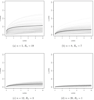
3.11 The error eΛ plotted against Λ, for 100 simulations from each of various complete tournaments onnplayers, repeated Rn times. The bold line gives the average ofeΛ across all 100 simulations. . . 37

4.1 A four-level model . . . 41

4.2 Illustration of some graph theory definitions . . . 42

(8)

4.4 Illustration of the notion of a chordal graph . . . 54

4.5 The posterior dependence graph after two different transformations in Example 4.4 . . . 55

4.6 The limit of estimators maximising sequential reduction

approxima-tions to the likelihood, for various k, in a repeated star tournament with n = 50, as R → ∞. In each case the dotted line is y = x, representing the limit of a consistent estimator. . . 59

4.7 Some tournament designs . . . 59 4.8 An importance sampling approximations to`(1.20,1.06), plotted against

the number of samples, N, on a logarithmic scale. The

sequen-tial reduction approximations for different k are overlaid, with x -coordinates chosen to give a time comparison between the two methods. 62

5.1 Construction of ˜yfor a complete tournament among 4 players . . . . 86

5.2 The densities of the true distributions for ui. The dotted line gives

(9)

Acknowledgments

I would like to thank my supervisor, David Firth, for giving me advice when I needed

it, for allowing me the time and freedom to develop my own ideas, and for careful

reading of this thesis.

I am grateful to Allesandra Salvan for allowing me to visit the Department

of Statistics at the University of Padua in November 2012, and to Cristiano Varin

for his hospitality during this visit, and for many useful discussions. The ADMB

software used for comparison in Chapter 4 was introduced to me by Cristiano Varin

and Manuela Cattelan at this time.

My thanks go to the many friends I have made here at Warwick over the

course of my PhD, for making this such an enjoyable time. I am hugely grateful to

my family, and in particular my husband Tom, for many years of love, support and

encouragement.

I acknowledge funding from the Engineering and Physical Sciences Research

(10)

Declarations

This thesis is submitted to the University of Warwick in support of my application

for the degree of Doctor of Philosophy. It has been composed by myself and has not

been submitted in any previous application for any degree.

The work presented was carried out by the author except where explicitly

(11)

Abstract

The likelihood for the parameters of a generalised linear mixed model involves an

integral which may be of very high dimension. Because of this apparent

intractabil-ity, many alternative methods have been proposed for inference in these models, but

it is shown that all can fail when the model is sparse, in that there is only a small

amount of information available on each random effect.

The sequential reduction method developed in this thesis seeks to fill in this

gap, by exploiting the dependence structure of the posterior distribution of the

random effects to reduce dramatically the cost of approximating the likelihood in

models with sparse structure. Examples are given to demonstrate the high quality

of the new approximation relative to the available alternatives.

Finally, robustness of various estimators to misspecification of the

random-effect distribution is considered. It is found that certain marginal composite

likeli-hood estimators are not robust to such misspecification in situations in which the

full maximum likelihood estimator is robust, providing a counterexample to the

no-tion that composite likelihood estimators will always be at least as robust as the

(12)

Chapter 1

Introduction

When constructing a regression model, it is rarely believed that the covariates recorded for each item really contain all the information about that item which

might affect the distribution of the response. This may be acknowledged in the

model by the addition of an error term in the regression for each item on its covari-ates. In the case that a single, separate, observation is made on each item, it is not

possible to distinguish the error in the regression for each item from the uncertainty

in the response given the predictor resulting from that regression. However, if multi-ple observations are made on some items, it is important to include an item-specific

error term in the model. A model including these extra error terms, called random

effects, is known as a mixed model.

If the original regression takes the form of a generalised linear model, then

the addition of random effects leads to a generalised linear mixed model. For

con-creteness, it is these models which are studied in this thesis, although many of the same ideas could be transferred to more general mixed models. Chapter 2 gives

a more in-depth introduction to generalised linear mixed models, including as an

example a class of models for competitions between pairs of players, which are used as the primary example throughout the thesis.

It is easy to write down the conditional likelihood of the parameters given

the value of the random effects. However, the random effects are treated as random variables, not fixed quantities, so in order to find the marginal likelihood, we must

integrate this conditional likelihood over the assumed distribution of the random

effects. Except in a few special cases, this integral has no analytical form, and direct numerical integration is not computationally feasible if there are a large number of

(13)

possible to simplify the integral.

In Chapter 2, a review of some of the alternative methods for inference in generalised linear mixed models is given. One class of approaches involves replacing

the likelihood with some approximation, for example using Laplace’s method or

importance sampling. However, these approximations can fail badly in cases where the structure of the model is sparse, in that only a small amount of information is

available on each random effect, especially when the response is discrete, and may

only take a small number of values. The poor quality of approximation can result in estimators with very poor statistical properties. Composite likelihood methods for

inference are also considered, and are shown to have low efficiency in many cases.

Chapter 3 considers in more detail the situations in which each alternative method of inference may be expected to perform well, and those in which they will perform

badly. A gap is discovered for some models with sparse structure, for which none of

the currently available methods appears to work well.

Chapter 4 introduces a new method of approximating the likelihood, called

the sequential reduction method, which is designed to bridge this gap. The main

idea of the method is to fully exploit the structure of the model in order to simplify the computation of the likelihood. This is done using ideas from the field of

graph-ical models, which are introduced at the start of the chapter. The new method is compared with existing approximation methods through numerical examples, and

is found to perform well in many cases. In particular, it is shown that the sequential

reduction method offers a great improvement over importance sampling approxima-tions for models with sparse structure.

Chapters 2-4 of the thesis consider the question of how best to conduct

in-ference in a generalised linear mixed model, under the assumption that the model is correctly specified. In Chapter 5, this assumption is partially dropped, and the

ro-bustness of various estimators to misspecification of the random-effects distribution

is studied. It is shown that estimators from composite likelihoods constructed using small blocks of components are inconsistent under misspecification of the

random-effects distribution in an asymptotic setting in which the maximum likelihood

esti-mator is consistent. A major motivation for the use of composite likelihoods is their potential for increased robustness compared to the full likelihood, so this result is

important as a warning that such increased robustness cannot be guaranteed. The

estimator from the sequential reduction approximation to the likelihood inherits the same robustness as the true maximum likelihood estimator, thereby providing

(14)

Chapter 2

Generalised linear mixed models

2.1 Generalised linear mixed models

2.1.1 The linear mixed model

Suppose that we wish to construct a regression model for a response Yi measured

on an itemi, based on some covariatesxi observed on that item. The simplest and

most well-studied of all such regression models is the linear model, in which it is

assumed that

Yi =βTxi+i,

wherei ∼N(0, τ2), and β and τ are unknown parameters. Writingηi =βTxi, so

that we model

Yi =ηi+i,

we could think ofηi as some underlying quantity about item iwhich is measured,

with error, byYi.

Now suppose that instead of making a single observation on each itemi, we makemi repeated observations

Yij, i= 1, . . . , n, j= 1, . . . , mi.

Thinking of each Yij as an imperfect measurement of ηi, we could model

Yij =ηi+ij,

whereij ∼N(0, τ2). If we still assume that

(15)

then the value of the observed covariate entirely determines the distribution of the

response. Put another way, if two items i and j have the same covariate values, then the responses for those items must have the same distribution.

This assumption is clearly unrealistic: there will undoubtedly be information

relevant to the response which is not encoded by the observed covariates. A more realistic model should acknowledge this extra uncertainty, letting

ηi =βTxi+bi,

wherebi represents the error in predicting ηi from the observed covariates. A

com-mon assumption is that bi is also a normal error term, so that bi ∼ N(0, σ2) for

some unknown parameterσ.

In the case thatmi= 1, so that there is only one observation on each item,

Yi =βTxi+bi+i,

where bi ∼ N(0, σ2) and i ∼ N(0, τ2), and bi and i are independent. There is

then no way to distinguish the errorbi in predictingηi givenxi, and the observation

error i. We may combine the two errors, to give ei = bi +i ∼ N(0, σ2 +τ2).

The parameters (σ, τ) are not separately identifiable. Instead, it is only possible to identify the combination ω2 =σ2+τ2. So in fact,

Yi=ηi+ei,

whereei∼N(0, ω2), and we have returned to the original linear model.

The case of repeated observations on each item is not the only one in which

it is important to recognise the heterogeneity between items with the same covariate value. Section 2.2 gives some more examples of settings in which it is possible to

detect the difference between the two types of error. In all of these settings, it is

important to include the extra error termbi, usually called a random effect, in the

model.

Writing the linear model in vector form, we have

Y =Xβ+,

where X is a known design matrix, and i ∼ N(0, τ2). To extend this to allow

heterogeneity between items with the same covariate values, we write

(16)

whereZ is a known design matrix for the random effects,b∼N(0, D(ψ)),andψ is an unknown parameter. This extension of the linear model, to include random effects bas well as fixed effectsβ, is known as a linear mixed model. Westet al.(2006) give

a brief history of the development of the linear mixed model. It turns out that full

likelihood inference for the linear mixed model remains relatively straightforward, as discussed in Section 2.3.2.

2.1.2 Mixed models in general

The same arguments for the addition of random effects to the linear model apply equally to any regression model, and lead to the definition of mixed models in

a more general setting. The class of generalised linear models provide a natural

extension to the linear model, and are widely used in practice. We now consider the addition of random effects to generalised linear models, which will lead us to

define the generalised linear mixed model. For concreteness, the focus of this thesis

will be these generalised linear mixed models, although many of the ideas are also applicable to mixed models outside of this framework.

2.1.3 The generalised linear mixed model

A generalised linear model (Nelder & Wedderburn, 1972) allows the distribution

of a response Y = (Y1, . . . , Ym) to depend on observed covariates through a linear

predictorη, where

η=Xβ,

for some known design matrixX. Conditional on knowledge of the linear predictor,

and possibly an unknown dispersion parameter τ, the components of Y are

inde-pendent, and the distribution of Y is fixed. The distribution of Y is assumed to have exponential family form, with mean

µ=E(y|η) =g−1(η),

for some known link functiong(.).

As in the linear model, an assumption implicit in the generalised linear model

is that the distribution of the response is entirely determined by the values of the observed covariates. In practice, this assumption is rarely believed: in fact, there

may be other information not encoded in the observed covariates which may affect

(17)

A generalised linear mixed model does this by modelling the linear predictor as

η=Xβ+Zb, (2.1)

where X and Z are known design matrices, and b is a sample from a

distri-bution known up to a parameter vector ψ. In most cases, it is assumed that

b ∼Nn(0, D(ψ)),and some methods rely on this assumption. The idea of adding

random effects to the the linear predictor in particular examples of generalised linear

models first appeared in the 1980s, for example for logistic regression for binary data

in Williams (1982) and for log-linear regression for Poisson data in Breslow (1984). Schall (1991) discusses the addition of random effects to an arbitrary generalised

linear model.

There are only a relatively small number of named multivariate distributions

to choose from for the distribution ofb. Instead, non-normalbcould be constructed

by taking

b=A(ψ)u, (2.2)

where the components of u are independent of one another, and may have any

univariate distribution FU(., ψ), possibly depending on the unknown parameter ψ.

Combining (2.1) and (2.2), we write

η=Xβ+Z(ψ)u, (2.3)

where ui ∼ FU(., ψ) and Z(ψ) = ZA(ψ). This thesis concentrates on the case in

which ui ∼ N(0,1), which allows b to have any multivariate normal distribution

with mean zero. The techniques described in Chapter 4 could be extended easily for use with other random effect distributions of the form (2.2).

The non-zero elements of the columns ofZ(ψ) give us the observations which

involve each random effect. We will say the generalised linear mixed model has ‘sparse structure’ if most of these columns have few non-zero elements, so that most

random effects are only involved in a few observations. These sparse models are

particularly problematic for inference, especially when the response may only take a small number of values, because the amount of information available on each random

(18)

2.2 Examples of generalised linear mixed models

2.2.1 Models with nested structure

Suppose that observations are recorded on items which are clustered into groups, so

that we havemi observations for each groupi= 1, . . . , n. Consider the model

ηij =β0+β1x(1)ij +. . .+βpx(ijp)+bi0,

where ij denotes the jth item in group i, for j = 1, . . . , mi,i= 1, . . . n, and bi0 ∼ N(0, σ2) is a group-level random effect. The addition of bi0 to the model allows

for the fact that there may be some error in prediction of ηij from the observed

covariates. The items contained within each group may share characteristics which are not observed, andbi0may be thought of as representing those unobserved shared

characteristics of group i. Write m = Pn

i=1mi for the total number of items.

Written in vector form,

η=Xβ+Z(σ)u,

whereX is anm×(p+ 1) matrix with rows

Xr= (1, x(1)irjr, . . . , x

(p)

irjr)

wherer is the jrth item in group ir. Them×n matrixZ(σ) has components

Zrs(σ) =







σ ifir=s

0 otherwise

. (2.4)

This model is called a two-level random intercept model. This is a sparse model if

the number of observations per group,mi, is small for most i.

In a three-level model, the groups themselves are clustered within larger groups. Models with even more levels can be built by repeatedly clustering the

top-level group within larger groups. It is also possible to allow for interaction between

the observed covariates and the random effects, leading to a model with random slopes, in addition to a random intercept. These are all examples of a wider class of

multilevel models, and many examples of such models may be found in Goldstein

(19)

2.2.2 Pairwise competition models

Consider a tournament among n players, consisting of contests between pairs of

players. Let yij record the outcome of a contest between players i and j. We

suppose that each player i has some ability λi, and that conditional on all the

abilities, the outcomes Yij are independent, with distribution depending on the

difference in abilities of the playersiand j, so that

E(Yij|λ) =g−1(λi−λj)

for some link functiong(.).

The pairwise competition models used as examples in this thesis all have bi-nary outcomes, so we observe only which player wins each contest. We consider these

binary models because each observation only provides a small amount of

informa-tion about the random effects, so approximainforma-tions to the likelihood are most likely to fail. Ifg(x) = logit(x), then this describes a Bradley-Terry model (Bradley & Terry,

1952). Ifg(x) = Φ−1(x) (the probit link), then it describes a Thurstone-Mosteller

model (Thurstone (1927), Mosteller (1951)).

If covariate informationxi is available for each player, then interest may lie

in the effect of the observed covariates on ability, rather than the individual abilities

λi themselves. For example, Whiting et al. (2006), conducted an experiment to

determine the effect of covariates on the fighting ability of Augrabies flat lizards,

Platysaurus broadleyi. The scientific hypothesis of interest was whether the

spec-trum of the throat of the lizard had an effect on fighting ability. To investigate this, Whiting et al. (2006) captured n = 77 lizards, recorded various measurements on

each, and then released them and recorded the outcomes of fights between pairs of

animals.

To model situations of this sort, suppose that the ability of a player may be

modelled as a linear function of their covariates, plus an error term, so that

λi =βTxi+bi

where thebi are independent samples from aN(0, σ2) distribution.

This may be written in generalised linear mixed model form by specifying thatE(Yij) =g−1(ηij), where

(20)

To write (2.5) in the form (2.3), we letXbe anm×pmatrix with components

Xrs=xp1(r)s−xp2(r)s

where p1(r) gives the first player involved in contest r, and p2(r) the second, and

wherexisis thesth component of the vector of observed covariates for playeri. Let

¯

Z be anm×nmatrix with components

¯

Zrs =



   

   

1 ifp1(r) =s

−1 ifp2(r) =s

0 otherwise

,

and writeZ(σ) =σZ¯. Then

η=Xβ+Z(σ)u,

whereu∼Nn(0, I).

Notice that the non-zero components of the sth column give the contests involving players, so the tournament will have sparse structure if most players only

compete in only a small number of contests.

Such a model for the flat-lizards tournament gives us an example of a gen-eralised linear mixed model with sparse structure, since we only observe a total of

100 contests among the 77 lizards.

2.2.3 Other pairwise interaction models

There are many other models with a similar structure to these pairwise competition

models, in that the outcome is determined by some interaction between pairs of

items. In fact, many of the generalised linear mixed models which have been noted to have intractable likelihoods fall into this class. For example, McCullagh & Nelder

(1989) give data gathered on pairs of salamanders from two separate regions. The

experiment consisted of attempts to mate each salamander with other salamanders from the same region, and with salamanders from the other region. The aim was to

determine whether two salamanders from different regions were less likely to mate

with one another than two salamanders from the same region.

In this case, the linear predictor is determined by sum of the individual

effects of each salamander, plus a term for the interaction between the region of the

(21)

predictor might be given by

ηij =βTxij+bMi +bFj,

wherebM_i ∼N(0, σ2_M) andbF_j ∼N(0, σ_F2), andxij contains the interaction between

the regions of the two salamanders. Written in vector form,

η =Xβ+Z(σM, σF)u,

where

Xr =xm(r)f(r),

where m(r) and f(r) are the male and female salamanders involved in mating

at-temptr, and

Zrs(σM, σF) =



   

   

σM ifm(r) =s

σF iff(r) =s

0 otherwise

.

2.3 Inference in generalised linear mixed models

2.3.1 The likelihood

Letf(.|ηi) be the density ofYi, conditional on knowledge of the value ofηi.

Condi-tional onη, the components of Y are independent, so that

L(β, ψ|y) = Z

Rn

m

Y

i=1

f yi|ηi=XiTβ+Zi(ψ)Tu

n

Y

j=1

φ(uj)duj, (2.6)

whereXi is the ith row ofX, and Zi(ψ) is theith row ofZ(ψ).

By using a product ofK-point quadrature rules, an n-dimensional integral may be approximated at cost O(Kn), where the error in the approximation tends to 0 as K → ∞. Unless n is very small, it will therefore not be possible to ap-proximate the likelihood well by direct computation of this integral using a product of quadrature rules. However, while the likelihood may always be written in form

(2.6), there are some occasions where it may be simplified, so that computation of an

n-dimensional integral is not necessary. Example 3.1 demonstrates such a simplifica-tion in one particular pairwise competisimplifica-tion model. The sequential reducsimplifica-tion method

developed in Chapter 4 gives a systematic way to check for such simplifications to

(22)

2.3.2 Laplace approximation to the likelihood

Many alternative methods of inference work by replacing the likelihood with some

approximation to it. The success of these methods depends on the quality of that

approximation. The Laplace approximation is a particularly simple approximation method.

Write

g(u1, . . . , un|y, β, ψ) = m

Y

i=1

f yi|ηi=XiTβ+Zi(ψ)Tu

n

Y

j=1 φ(uj)

for the integrand of the likelihood. This may be thought of as a non-normalised

version of the posterior density foru, given y,β and ψ.

Pinheiro & Bates (1995) suggest using a Laplace approximation to this

in-tegral. For each fixed θ = (β, ψ), the Laplace approximation approach relies on a

normal approximation to the posterior density of u, given y and θ. To find this normal approximation, letuˆθ maximise

logg(u|y, θ)

overu, and let Hθ =Hθ(ˆu) be the Hessian resulting from this optimisation, where

Hθ(u) =∇u∇Tulogg(u|y, θ).

The normal approximation tog(.|y, θ) will be proportional to aNn(ˆuθ, H_θ−1) density.

Writinggna(.|y, θ) for the normal approximation to g(.|y, θ),

gna(u|y, θ) = g(ˆuθ|y, θ)

φn(ˆuθ;ˆuθ, Hθ−1)

φn(u;ˆuθ, Hθ−1),

where we writeφn(.;µ,Σ) for the Nn(µ,Σ) density.

When we integrate overu, only the normalising constant remains, so that

˜

L(θ|y) = g(ˆuθ|y, θ)

φn(ˆuθ;uˆθ, H_θ−1)

= (2π)−n2(detH_θ)− 1

2g(ˆu_θ|y, θ).

In the case of a linear mixed model,

g(u|y, θ) =

m

Y

i=1 φ

X_iTβ+Zi(ψ)Tu−yi

τ

n

Y

j=1 φ(uj),

(23)

nor-mal density is precise, and there is no error in the Laplace approximation to the

likelihood. In other cases, and particularly when the response is discrete and may only take a few values, the error in the Laplace approximation can be large.

Validity of the Laplace approximation

Recall that we have n random effects, and m observations, so that the likelihood

may be written as an n-dimensional integral over a integrand containing a product of m terms. In the case that n is fixed, and m → ∞, the relative error in the Laplace approximation may be shown to tend to zero. However, in the type of

model we consider here, n is not fixed, but grows with m. The validity of the Laplace approximation depends upon the rate of this growth. Shun & McCullagh

(1995) study this problem, and conclude that the Laplace approximation should be

reliable, provided thatn=o(m1/3). If ngrows with mmore quickly than o(m1/3), the relative error in the Laplace approximation may beO(1). These rates are rather

slower than those which are typical of the type of models considered here, in which

a sparse model may have n = O(m) (see Example 3.2), and where we consider a model with n=O(m1/2) to have dense structure (see Example 3.5).

However, the Laplace approximation to the difference in the log-likelihood

at two nearby points tends to be much more accurate than the approximation to the log-likelihood itself, and in denser models, where there is more information

available per random effect, the Laplace approximation to the shape of the likelihood

appears to be sufficiently good to give accurate inference, even in cases where the approximation to the likelihood itself has large relative error. See Example 3.5 for

a demonstration of this, in a situation with n = O(m1/2). The effect that ratios of Laplace approximations to similar functions tend to be more accurate than each Laplace approximation individually has been noted before, for example by Tierney

& Kadane (1986) in the context of computing posterior moments. However, in

models with very sparse structure, even the shape of the Laplace approximation may be inaccurate, so another method is required. The behaviour of the Laplace

approximation in models with differing levels of sparsity is studied in Chapter 3.

Other methods based on the Laplace approximation

Many alternative methods for inference in a generalised linear mixed model are based on a Laplace approximation to the likelihood. For instance, Breslow & Clayton

(1993) base their Penalised Quasi Likelihood (PQL) on a further approximation

(24)

is not suitable for inference in models for binary data, with a small number of

observations for each random effect. Browne & Draper (2006) consider an example of such a model, and show that PQL gives highly biased estimators and confidence

intervals with low coverage in that case.

2.3.3 Importance sampling approximation to the likelihood

Recall that the likelihood may be written as an integral

L(θ|y) = Z

Rn

g(u|y, θ)du, (2.7)

where g(.|y, θ) may be approximated by a function gna(.|y, θ) proportional to the density of a Nn(µθ,Σθ) distribution. Replacing g(.|y, θ) with gna(.|y, θ) in (2.7)

yields the Laplace approximation to the likelihood.

In cases where the Laplace approximation fails, Pinheiro & Bates (1995)

sug-gest constructing an importance sampling approximation to (2.7), based on samples from the approximating normal distributionNn(µθ,Σθ). Writing

w(u;θ) = g(u|y, θ)

φn(u;µθ,Σθ)

,

the likelihood may be written as

L(θ|y) = Z

Rn

w(u;θ)φn(u;µθ,Σθ)du

=E[w(U;θ)],

where U ∼ N(µθ,Σθ). This may be approximated by the importance sampling

approximation

LIS(θ|y) = 1

N

X

i=1

w(u(i);θ),

whereu(i)∼N(µθ,Σθ).

By the weak law of large numbers,

LIS(θ|y)→p L(θ|y)

as N → ∞. Provided that σ_W2 = Var (w(U;θ)) < ∞, the central limit theorem implies that

√

(25)

as N → ∞. So, if the importance weights w(U;θ) have finite variance, the error in the importance sampling approximation shrinks at rate √N, irrespective of the dimensionnof the integral.

Unfortunately, there is no guarantee that the variance of the importance

weights will be finite. It is difficult to check this theoretically in most practical applications, but in some situations where the normal approximation to g(.|θ) is poor, it appears that the variance is not finite (see Example 3.2). In such a situation,

the weak law of large numbers still holds, so the importance sampling approximation will still converge to the true likelihood, but the convergence may be slow and erratic,

and estimates of the variance of the approximation may be unreliable.

Interest lies in approximating the likelihood surface, rather than just the likelihood at a single pointθ. If a new random sampleu(1), . . . ,u(N)fromNn(µθ,Σθ)

is used for eachθ, the resulting approximation to the likelihood surface will be quite

rough. To ensure a smooth surface, Pinheiro & Bates (1995) suggest sampling t(i)∼Nn(0, I), and letting

u(i) =µθ+Aθt(i)

for eachθ, whereAθ is the Cholesky decomposition of Σθ.

2.3.4 Composite likelihood

If we had only some small subsety(s) of the observations, where y(s) only depends

on a small number, ds, of random effects, then we could evaluate the likelihood

L(θ|y(s)) via an integral of dimensionds.

The idea of a marginal composite likelihood (Lindsay, 1988) is to split the data up into blocks{y₍_s₎}K

s=1so that the likelihood based on each block is reasonably

easy to compute. A marginal composite likelihood based on these blocks may be

defined as

LC(θ) =

K

Y

s=1

L θ|y₍_s₎ws

,

wherews is a weight given to block s.

For instance, for inference in a pairwise competition model, Cattelan & Varin (2010) suggest using the blocks yijk = (yij, yik) of pairs of contests which share a

common player, with weightsws= 1 for alls.

For an appropriate choice of blocks, this method is fairly fast, and results on the consistency and asymptotic normality of the estimators are available in some

settings. A review of these results is given in Chapter 3. However, in many cases

(26)

maximum likelihood estimator. This is demonstrated in Example 3.1. It is also

often difficult to decide which blocks of componentsy(s) and weights ws to use to

construct the composite likelihood in any given setting. Cox & Reid (2004) and

Lindsayet al.(2011) give some initial ideas on answering these questions, but there

is currently no general-purpose method available for selection of good blocks of components and weights.

Composite likelihood is usually used mainly for computational reasons, but a

secondary motivation is given by the fact that only the marginal distributions of the blocks used in the composite likelihood need to be specified, rather than requiring

specification of the full joint distribution of the response vector. Varinet al.(2011)

and Xu & Reid (2011) discuss the potential this gives for increased robustness of the composite likelihood estimator relative to the full maximum likelihood

estima-tor. However, in Chapter 5 we find that in the context of generalised linear mixed

models, certain marginal composite likelihood estimators will be less robust to mis-specification of the random effects distribution than the full maximum likelihood

estimator.

2.3.5 Bayesian inference

Given a prior distributionπ(θ) for the parameter-vectorθ, the posterior distribution

ofθ is given by

π(θ|y)∝L(θ|y)π(θ).

If we were able to obtain a good approximation to the likelihood, then this could be

used to approximate the posterior distribution. However, in the case when no such approximation is readily available, Markov chain Monte Carlo methods may be used

to find samplesθ(i) whose distribution converges to the posterior, once a sufficiently

large number of samples have been taken. Zeger & Karim (1991) describe how such samples may be obtained by Gibbs sampling in the case of a generalised linear mixed

model.

Such methods have their problems, primarily that it can sometimes take a long time for the convergence to the posterior distribution to occur, and it is difficult

to check when this convergence has taken place.

To construct the posterior distribution, it is necessary to choose a prior distribution forθ. In models with binary response and sparse structure, the choice

of prior distribution for the parameters of the random effects distribution often

(27)

posterior distribution (Hobert & Casella, 1996).

There is certainly much more to be said about Bayesian methods for inference for generalised linear mixed models, but they are not directly discussed further in

this thesis. The focus is instead on approximations and alternatives to the likelihood,

(28)

Chapter 3

Performance of existing

methods of inference

3.1 Asymptotics under independent replication

3.1.1 Estimating equations

In the simple asymptotic framework of an increasing number, R, of independent

replications, the maximum likelihood estimator is consistent and normally dis-tributed in the limit as R → ∞, as long as certain regularity conditions hold. Provided that analogues of these conditions continue to hold, and in particular that

the parameter of interest is identifiable from the composite likelihood, the compos-ite likelihood estimator is also consistent and asymptotically normal as R → ∞. The variance of the limiting distribution of the composite likelihood estimator is

larger than that of the maximum likelihood estimator, except in cases where the two estimators are identical.

These results apply in a general setting, not just in the case of generalised

linear mixed models. They can be shown by applying the theory of estimating equations, which is now reviewed. These results will be applied several times in

the thesis, for example to provide results on the asymptotic behaviour of composite likelihood estimators, and of estimators found by maximising an approximation to

the likelihood, rather than the likelihood itself.

(29)

estimator ofθ solving the estimating equation

vR(θ,y) = R

X

i=1

v(1)(θ,y(i)).

For instance, in the case of full likelihood, v(1)(θ,y(i)) would be the score function

associated with observingy(i), and vR(θ,y) the overall score function for y. Let

¯

v(θ) =E[v(1)(θ;Y)],

where the expectation is taken over the true distribution of eachY(i).

Theorem 1. Suppose that v¯(.) is a continuous function of θ, with unique root θ∗.

Suppose that Θis compact, that v(1)(θ,y) is a continuous function of θ for each y,

and that

v(1)(θ,y)

≤g(y)

for some integrable functiong, for allθ in a neighbourhood of θ∗. Then

ˆ

θR→pθ∗

as R→ ∞, where →p _{denotes convergence in probability.}

Proof. See van der Vaart (1998, pp. 44–46)

With a few extra conditions, results on the asymptotic normality of ˆθR may

also be obtained.

Let

H(θ) =E−∇θv(1)(θ,Y)

and

J(θ) =E h

v(1)(θ,Y)

Ti

.

Theorem 2. Suppose that the conditions assumed in Theorem 1 hold, and in

addi-tion that v₍₁₎(θ,y) has continuous second derivatives for each y, and

∂2v₍₁₎(θ,y)

∂θi∂θj

≤h(y)

for some integrable functionh, for allθ in a neighbourhood of θ∗. Then

√

R(ˆθR−θ∗)→dNp(0, H(θ∗)−1J(θ∗)

(30)

as R→ ∞, where →d _{denotes convergence in distribution.}

Proof. See van der Vaart (1998, pp. 51–52)

Note. The regularity conditions given in the statement of Theorems 1 and 2 are

stronger than are needed. See van der Vaart (1998, pp. 46–47, 52–53) for some

weaker conditions which could be used instead.

3.1.2 Maximum likelihood estimator

We may show the consistency and asymptotic normality of the maximum likelihood

estimator ˆθR by application of these results to the score function

u(θ|y) =∇_θ`(θ|y).

Let

¯

u(θ) =E[u(θ|Y)].

Suppose that the model for the data is correct, so that y(1), . . . ,y(R) really are

samples from the assumed distribution, for some valueθ0 of θ. Assuming sufficient

further regularity conditions to allow interchange of differentiation and integration,

the first Bartlett identity

¯

u(θ0) = 0 (3.1)

may then be shown to hold. Assuming that this root is unique, and that the other

regularity conditions of Theorems 1 and 2 hold withv(1)(θ,y) =u(θ|y), we obtain

that

ˆ

θR→pθ0,

so the maximum likelihood estimator is consistent, and

√

R(ˆθn−θ0)→dNp(0, H(θ0)−1J(θ0)

H(θ0)T

−1

) (3.2)

asR → ∞. In this case, the second Bartlett identity gives thatH(θ0) =J(θ0), and

we call this quantity the Fisher information matrix, denoted by I(θ0). Equation

(3.2) then simplifies to the familiar

√

(31)

3.1.3 Composite likelihood estimator

The results can also be applied to show consistency and asymptotic normality of

the composite likelihood estimator ˆθC_R. Writing

uC(θ|y) =∇θ`C(θ|y).

for the composite score function, let

¯

uC(θ) =E[uC(θ|Y)].

Note that

¯

uC(θ) =E∇θ`C(θ;Y)

=E

" _K

X

s=1

∇θ`(θ;Y(s))

#

=

K

X

s=1

E∇θ`(θ;Y(s))

.

So if the model is correct withθ=θ0, thenuC(θ0) = 0, since the expectation of each

score in the sum is 0, by (3.1). If this solution is unique, and the other regularity

conditions of Theorems 1 and 2 hold withv(1)(θ,y) =uC(θ|y), then

ˆ

θC_R →p _θ

0,

and

√

R(ˆθC_R−θ0)→dNp(0, HC(θ0)−1JC(θ0)

HC(θ0)T

−1

)

asR → ∞. This time, there is no simplification in the variance term, since the sec-ond Bartlett equality does not hold. We write GC(θ0) =HC(θ0)TJC(θ0)−1HC(θ0). GC(.) is known as the Godambe or sandwich information matrix. The asymptotic

variance of the composite likelihood estimator is in general larger than that of the

full likelihood estimator. In the scalar-parameter casep= 1, it is sometimes useful to consider theasymptotic relative efficiency

r = avar(ˆθR) avar(ˆθC_R) =

[HC(θ0)]2 I(θ0)JC(θ0)

∈(0,1].

(32)

1

2

3

4

5

6

. . . . . . n−1

[image:32.595.205.406.74.279.2]

n

Figure 3.1: A star tournament on nplayers

model, in which the ability of a player is modelled as

λi =σui,

where ui ∼ N(0,1), and σ is the unknown parameter of interest. That is, we

are interested in the overall spread of abilities among players. Conditional on the

abilities, we assume thatP r(ibeats j) = Φ(λi−λj).

This model is simpler than most pairwise competition models of practical

interest, in which we model the effect of some observed covariates on the ability of

a player. However, because of the simplicity of this model, it is relatively easy to study some statistical properties of the various estimators considered in Section 2.3.

If an estimator of σ in this simple model has poor properties, there is little hope

that the corresponding estimator will be successful in a more complex model. In order for the asymptotic regime described above to apply, we assume

that the tournament consists of R repetitions of a smaller tournament with fixed

structure, and consider what happens in the limit atR→ ∞. We assume that the small tournaments each have an ‘star’ structure, as shown in Figure 3.1. We allow

the number of playersn in each star to vary, and consider how the the asymptotic

relative efficiency of the pairwise likelihood estimator changes as it does so.

Figure 3.2 is a plot of the asymptotic relative efficiency of the pairwise

like-lihood estimator relative to the maximum likelike-lihood estimator, for a repeated star

tournament for various values of n. In the case n = 3, the pairwise likelihood is identical to the full likelihood, and so the pairwise likelihood estimator is fully

(33)

10 20 30 40

0.0

0.2

0.4

0.6

0.8

1.0

n

asymptotic relativ

[image:33.595.165.475.112.305.2]

e efficiency

Figure 3.2: The asymptotic relative efficiency of the pairwise likelihood estimator ofσ, in a repeated star tournament for various values of n.

estimator drops quickly. For large n, there is a large drop in efficiency incurred by

using this pairwise likelihood instead of the full likelihood, and it seems sensible to

try using some approximation to the likelihood instead.

Note. The structure of the tournament in Example 3.1 was chosen to make it easy to obtain the limiting distributions of the various estimators. In the case of the star

tournament, it is possible to simplify the likelihood, by noting that conditional on

the value of the random effect for the central player in the star, the contests are independent. This means that the likelihood for a star onnplayers may be written

as

L(σ|y) =

Z ∞

−∞

" _n

Y

i=2

Z ∞

−∞

Φ σ(ui−u1)(−1)yi1+1

φ(ui)dui

#

φ(u1)du1.

In fact,

Z ∞

−∞

Φ σ(ui−u1)(−1)yi1+1

φ(ui)dui = Φ

σu_√1(−1)yi1

1 +σ2

,

so the likelihood can be computed by evaluating a single one-dimensional integral.

By differentiating under the integral, the first and second derivatives of the likelihood

with respect toσ are also easy to compute.

The example also has a lot of symmetry, and a sufficient statistic forσ isW1,

the number of times the central player in the star wins. In fact, we would make the

same inference aboutσ whether we observed the central player to winw1 times, and

(34)

So

S1 = min{W1, n−1−W1} ∈

0,1, . . . ,

jn−1

2

k

is a sufficient statistic for σ. It is straightforward to enumerate all the possibilities

forS1, and to find the probability of each occurring under the model. By computing

the likelihood and its derivatives, and the pairwise likelihood and its derivatives, for

a tournament corresponding to each choice of S1, it is therefore possible to find

the asymptotic variance of the full likelihood estimator, and that of the pairwise likelihood estimator.

3.1.4 Estimators maximising an approximation to the likelihood

Many of the methods for inference considered in Chapter 2 involve replacing the like-lihood with some approximation to it. The estimators obtained by maximising this

approximated likelihood need no longer be consistent as the number of independent

replications tends to infinity. Suppose that the approximation to the log-likelihood is smooth, so that we have an approximation ˜u(θ|y) to the score function given datay. The resulting estimator ˜θRmaximising the approximation to the likelihood

solves

R

X

i=1

˜

u(θ|y₍_i₎) = 0.

Let ˜θ be the solution to

E[˜u(θ|Y)] = 0,

where the expectation is taken under the true distribution. Then, applying Theorem

1,

˜

θR→p θ˜

asR→ ∞.

Applying Theorem 2 gives that

√

R(˜θR−θ˜)→dNp

0,H˜(˜θ)−1J˜(˜θ)hH˜(˜θ)Ti

−1

.

However, by treating the approximation to the likelihood as if it were the true

likelihood, we will assume that, for largeR,√R(˜θn−θ0) is well approximated by a

normal distribution, with variance the inverse of the observed information matrix of the approximated likelihood at its maximum ˜θR. So, as the estimator tends towards

˜

θ, we are more and more sure that the estimator is close to θ0. If ˜θ 6= θ0, this

(35)

nominal level.

If the approximation to the likelihood is sufficiently good, ˜θwill be very close to θ0, and the confidence regions for θ will have approximately correct coverage

provided that R is not extremely large. However, poor-quality approximations can

result in an estimator with a very large asymptotic bias, as Example 3.2 shows.

Example 3.2. We return to the star tournaments of Example 3.1. Recall that the ability of playeriis modelled as

λi =σui,

whereσ is an unknown parameter of interest. Now we suppose that we do inference by replacing the likelihood with an approximation, found either by using Laplace’s

method or by importance sampling. Recall that in the limit as the number of repetitions,R, tends to infinity, the maximum likelihood estimator and the pairwise

likelihood estimator are both consistent. This will not be true for the estimators

found by maximising approximations to the likelihood, so we are interested in how far the limits of the estimators are from the true value in each case.

Suppose that the number of players in each tournament, n, is fixed at 50.

First, we consider the effect of using the Laplace approximation to the likelihood in place of the true likelihood. Figure 3.3a shows the limit of the estimator maximising

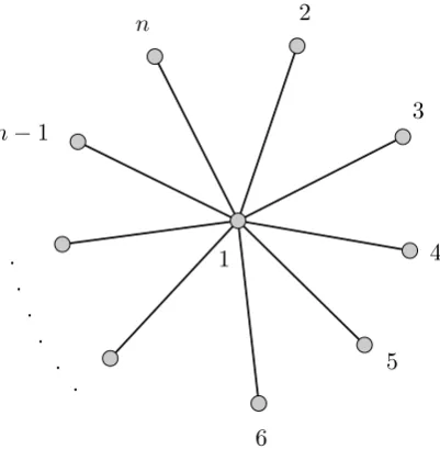
the Laplace approximation to the likelihood, plotted against the true value of σ.

Even for quite small values of σ, there is a large negative asymptotic bias in the Laplace estimator ofσ.

The Laplace approximation performs badly in this case, so we might instead

choose to use an importance sampling approximation to the likelihood. This re-quires N evaluations of the function g(.|y, θ), in addition to those required to find the normal approximation. Thus the method will be considerably more expensive

than using a quadrature rule to compute the one dimensional integral in the sim-plified version of the likelihood, even for small N. Nonetheless, the method is still

reasonably fast for small N, and importantly it is possible to use the method for

inference in any generalised linear mixed model, where the simplification afforded by the special structure of this case is not available.

Figure 3.3b shows the limit of an importance sampling estimator, where

the approximation is constructed based on one particular random sample of size

N = 104, using the same samples to approximate the likelihood for each possible

observed tournament. The limit of the estimator would change if a different random

(36)

0.0 0.5 1.0 1.5 2.0 2.5

0.0

0.5

1.0

1.5

2.0

2.5

sigma0

limit of estimator

(a) Laplace

0.0 0.5 1.0 1.5 2.0 2.5

0.0

0.5

1.0

1.5

2.0

2.5

sigma0

limit of estimator

(b) Importance sampling (Using one sample of size N = 104₎

0.0 0.5 1.0 1.5 2.0 2.5

0.0

0.5

1.0

1.5

2.0

2.5

sigma0

limit of estimator

[image:36.595.183.454.120.617.2]

(c) Importance sampling (Using one sample of sizeN = 105₎

Figure 3.3: The limit of various estimators in a repeated star tournament with

(37)

0 5 10 15 20

0.00

0.01

0.02

0.03

0.04

0.05

S1

frequency

(a)σ= 1.3

0 5 10 15 20

0.00

0.01

0.02

0.03

0.04

0.05

S1

frequency

[image:37.595.149.493.113.350.2]

(b)σ= 2.5

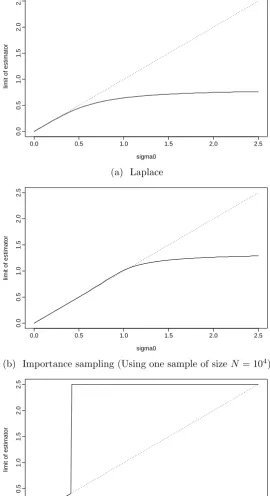
Figure 3.4: The distribution of S1 in a star tournament on n = 50 players, for

different values of σ.

The importance sampling approximation seems to offer a real improvement

over the Laplace approximation, but there is still a large asymptotic bias for mod-erate to large values ofσ.

Whenσ0= 2.5, the limit of this importance sampling estimator is 1.3. This

limiting value itself is moderately large, and since the distribution of tournaments will be very similar for all σ sufficiently large, it seems possible that the practical

effects of this asymptotic bias will be small. However, Figure 3.4 shows that there is

a noticeable difference in behaviour between the distribution ofS1 forσ = 1.3 and σ= 2.5, so the difference is an important one.

It is worth seeing what happens when we use an even larger number of

samplesN to construct the importance sampling approximation. The limit of the estimator for one particular sample of size N = 105 is shown in Figure 3.3c. The

asymptotic bias of the estimator is now much larger than in the N = 104 case.

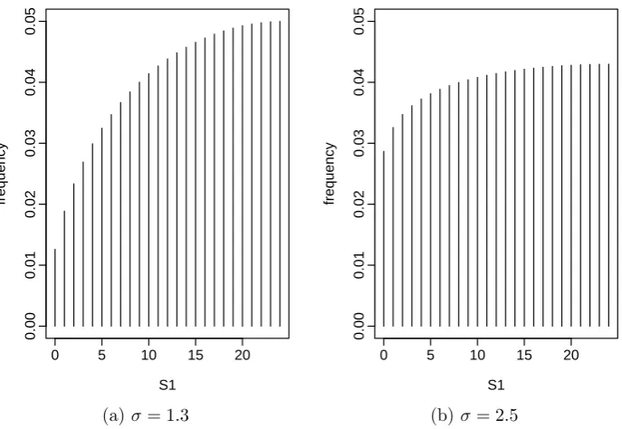
Examining the shape of the approximation for N = 105 for S1 = 15 in Figure

3.5, we can see that the approximated log-likelihood for large σ is much too large.

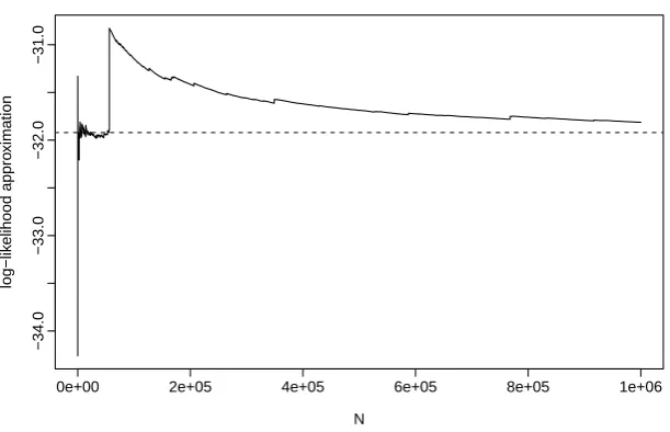
Figure 3.6 shows a trace plot of the log-likelihood approximation for S1 = 15 and

σ = 2, using from one up to 106 samples. There is a large jump in the likelihood approximation at around N = 105, after the approximation has already appeared

(38)

0.0 0.5 1.0 1.5 2.0 2.5

−34.0

−33.0

−32.0

−31.0

sigma

log−lik

[image:38.595.165.474.113.305.2]

elihood

Figure 3.5: An importance sampling approximation to the log-likelihood for a star tournament with S1 = 15, using N = 105 samples. The dotted line gives the true

log-likelihood.

finite variance, which, as discussed in Section 2.3.3, can lead to slow and unstable convergence of the approximation.

3.1.5 Hypothesis testing and confidence intervals

It will generally be of interest not just to obtain point estimates for the parameters

of a generalised linear mixed model, but to test hypotheses about these parameters, or to construct confidence intervals for them.

Suppose that we have ap-dimensional parameter vectorθ, and consider

test-ing the hypothesisφ=φ0 for somep0-dimensional subset φof θ.

We will consider two test statistics for testing such hypotheses, first assuming

that the true likelihood and the corresponding maximum likelihood estimator ˆθ are

available. Write ˆφfor maximum likelihood estimator ofφ, andIφφ(ˆθ) =hI(ˆθ)−_φφ1i−1,

whereI(ˆθ)−_φφ1 is the submatrix ofI(ˆθ)−1 corresponding toφ. The Likelihood ratio test statistic is defined as

Λ(φ0) = 2

"

sup

θ

`(θ|y)− sup

θ:φ=φ0

`(θ|y) #

,

and Wald test statistic as

(39)

0e+00 2e+05 4e+05 6e+05 8e+05 1e+06

−34.0

−33.0

−32.0

−31.0

N

log−lik

elihood appro

[image:39.595.167.473.110.307.2]

ximation

Figure 3.6: A trace of the importance sampling approximation to the log-likelihood at σ = 2, for a star tournament with S1 = 15. The dotted line gives the true

log-likelihood.

Under standard regularity conditions, it can be shown that under the null hypothesis thatφ=φ0, both Λ(φ0)→dχ2p−p0 and W(φ0)→dχ2p−p0 asR→ ∞.

However, one of the regularity conditions needed to prove these results is

sometimes violated in a generalised linear mixed model. Ifφ0 is on the boundary of

the parameter space, the standard asymptotic distribution of the test statistics need

not apply. Recall that in our definition of a generalised linear mixed model, there is

a parameterψcontrolling how the random effects enter into the linear predictor. We suppose thatψ= 0 corresponds to the case in which there are no random effects in

the model. If we are interested in testingψ= 0, then the parameter value of interest

is on the boundary of the parameter space. In this sort of situation, Self & Liang (1987) show that, if there are an increasing number of independent and identically

distributed observations, Λ has limiting distribution which is a mixture between the

usual χ2_p−p0 distribution and a point mass at 0. In practice, this means that some

adjustment should be made to the assumed null distribution of the test statistic if

the distribution under the null is such that the maximum likelihood estimator will

be on the boundary of the parameter space a non-negligible proportion of the time. In the more realistic setting in which the replications are not identically distributed,

Crainiceanu & Ruppert (2004) show that using a mixture betweenχ2_p₋_p₀distribution and a point mass at 0 may itself be incorrect. They demonstrate how to find the correct distribution of the likelihood ratio test statistic in a linear mixed model, but

(40)

models.

Throughout the remainder of the thesis, the unadjusted χ2_p₋_p₀ distributed will be used. This will result in a slight over-reluctance to reject the hypothesis that

ψis small.

To construct a confidence interval (or region, if p0 >1) for φ with

approxi-mate coverage 1−α, we can invert the hypothesis test, giving a Wald-type confidence region of

I_W(1−α)={φ:W(φ)≤cα}

and a likelihood ratio confidence region of

I_Λ(1−α)={φ: Λ(φ)≤cα},

wherecα is chosen so that P r(χ2p−p0 > cα) =α.Writing`

p₍_φ

0|y) = supθ:φ=φ0`(θ|y)

for the profile log-likelihood ofφ0, the the likelihood ratio statistic may be written

as

Λ(φ0) = 2

h

`p( ˆφ|y)−`p(φ0|y)

i

,

and the likelihood ratio confidence region

I_Λ(1−α) =nφ:`p(φ|y)≥`p( ˆφ|y)−cα

2 o

is just a set of points with sufficiently large profile likelihood.

The Wald test statistic is usually considerably easier to compute than the likelihood ratio test statistic. However, it exhibits worrying behaviour in some

settings. Hauck & Donner (1977) demonstrate the phenomenon that, as the true value of a regression parameter in a logistic regression model increases, the power of

the hypothesis test for testing that it is zero eventually starts to fall. Example 3.3

demonstrates similar behaviour for the variance parameter of the random effects in a generalised linear mixed model.

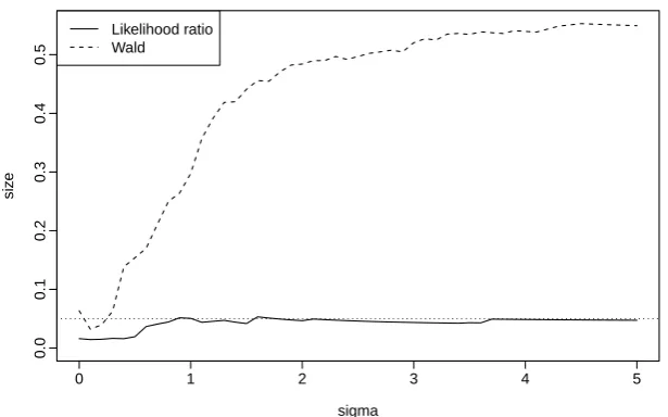
Example 3.3. Suppose that we have 3 replications of a star tournament on 50

players, as described in Example 3.1, and consider testingσ=σ0, for various values

of σ0. We construct Wald and likelihood ratio tests of nominal size α = 0.05. The

true sizes of these tests are given in Figure 3.7. The Wald test has size much larger

than the nominal size for most values ofσ0. On the other hand, the likelihood ratio

test has size smaller than 0.05 for σ very small (since no adjustment was made for the fact that the parameter is close to the boundary), but for largerσ has the correct

size.

(41)

0 1 2 3 4 5

0.0

0.1

0.2

0.3

0.4

0.5

sigma

siz

e

[image:41.595.166.474.112.304.2]

Likelihood ratio Wald

Figure 3.7: The true size of hypothesis tests forσ, of nominal size 0.05, in a repeated star tournament withn= 50,R = 3.

A similar phenomenon to that observed by Hauck & Donner (1977) may be seen

here: the power of the Wald test for testingσ= 0 diminishes for largeσ.

We conclude that the use of the Wald test statistic may be very misleading,

and it is far better to use the likelihood ratio test statistic.

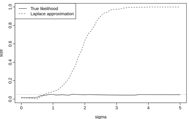
All of the above discussion relates to the situation in which the likelihood

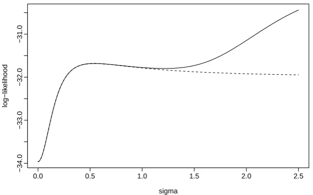
itself is available. When the likelihood is replaced by an approximation, the quality

of inference from the likelihood ratio test will depend on the quality of that ap-proximation. Figure 3.9 shows the true size of the approximate likelihood ratio test

constructed by using the Laplace approximation, in the repeated star tournament

described in Example 3.3. As expected, the size of the test for largeσis much larger than the nominal level.

When a composite likelihood is used in place of the full likelihood, the

asymp-totic distribution of the test statistics is no longerχ2_p−p0. A replacement composite

likelihood Wald test statistic could be constructed as

WC = ( ˆφC −φ0)TG_Cφφ(ˆθC)( ˆφC −φ0),

whereGφφ_C (ˆθC) =hGC(ˆθC)−_φφ1

i−1

and GC(ˆθC)−_φφ1 is the submatrix of the estimated

variance matrix hGC(ˆθC)

i−1

corresponding to φ. Varin et al. (2011) review some

of the different adjustments to the likelihood ratio test statistic which have been

(42)

0 1 2 3 4 5

0.0

0.2

0.4

0.6

0.8

sigma

po

w

er

[image:42.595.167.473.145.340.2]

Likelihood ratio Wald

Figure 3.8: The power of hypothesis tests of σ = 0, of nominal size 0.05, in a repeated star tournament withn= 50,R= 3.

0 1 2 3 4 5

0.0

0.2

0.4

0.6

0.8

1.0

sigma

siz

e

True likelihood Laplace approximation

[image:42.595.168.474.455.648.2]

(43)

drop in efficiency in the pairwise likelihood estimator is unacceptably large in some

circumstances.

3.1.6 Penalised forms of the likelihood

In sparse models with binary data, it is fairly common that the maximum likelihood

estimator is not finite. To prevent such problems, it seems sensible to impose some

penalty on the parameters.

In the case of a generalised linear model, where there are no random effects,

Firth (1993) demonstrates how to choose a penalty to remove the first-order asymp-totic bias in ˆβ. The penalty suggested here is equal to that bias reduction penalty,

chosen under the assumption of no random effects.

Write

I0(β) =E−∇Tβ∇β`(β, ψ= 0)

,

whereψ= 0 corresponds to the case of no random effects, and consider the penalised

likelihood

`p(β, ψ) =`(β, ψ)−p0(β),

where

p0(β) =−

1

2log|I0(β)|.

We call p0(.) the bias reduction penalty in all cases, although it removes the

first-order asymptotic bias only whenψ= 0.

We may use the penalised likelihood in place of the full likelihood to test

hypotheses using the Wald or likelihood ratio tests, because as the amount of infor-mation on the parameters in the data increases, the influence of the penalty term

shrinks, and the test statistics retain the same limiting distributions.

We will usep0(.) as a penalty in some of the examples in the thesis, and it

avoids infinite parameter estimates in those cases, but we do not claim that this

penalty is optimal in any way. It may be useful to additionally impose some penalty

onψ, or to construct a joint penalty onβ andψ, so that a larger penalty is given to parameter values whereβ is small butψis large. One idea for an improved penalty

function is given in Section 6.2.2, but some further work is required to check whether

(44)

. . .

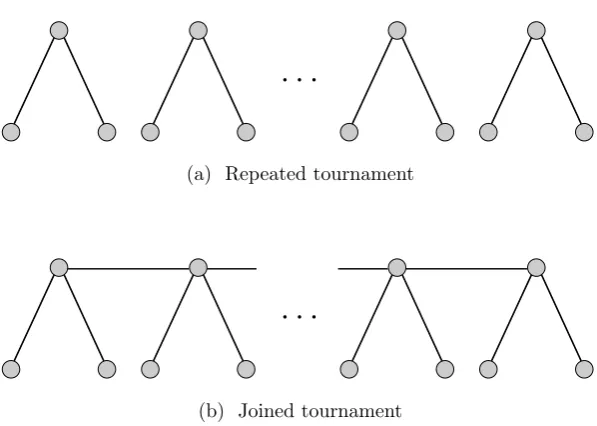
(a) Repeated tournament

. . .

[image:44.595.170.469.132.345.2]

(b) Joined tournament

Figure 3.10: Tournament designs for Example 3.4

3.2 Asymptotics without independent replication

In reality, we cannot rely on having a large number of independent replications of the

data. It is common to have few, or no, independent replications. Instead, we often

have a large number of observations, all dependent on one another. We still want to use the sort of results deduced underR→ ∞ asymptotics, such as the consistency and asymptotic normality of the maximum likelihood estimator. Assuming that

there is no independent replication, will these results still hold?

Example 3.4. ConsiderR repetitions of a star tournament on 3 players, as shown

in Figure 3.10a. Suppose again that

λi =σui,

whereui ∼ N(0,1) and σ is an unknown parameter. We have already shown that

the maximum likelihood estimator ofσ will be consistent in this setting as R→ ∞. For largeR, the maximum likelihood estimator ofσwill be approximately normally

distributed, with variance V_R, for some constant V. The total number of contests is such a tournament ism = 2R, and we could equally well speak of asymptotics as

m→ ∞.

Now consider a new tournament is which an additional contest is played