Performance engineering unstructured mesh, geometric multigrid codes

(1)

warwick.ac.uk/lib-publications

A Thesis Submitted for the Degree of PhD at the University of Warwick

Permanent WRAP URL:

http://wrap.warwick.ac.uk/89503

Copyright and reuse:

This thesis is made available online and is protected by original copyright.

Please scroll down to view the document itself.

Please refer to the repository record for this item for information to help you to cite it.

Our policy information is available from the repository home page.

(2)

M A

E

G

NS I

T A T MOLEM

U N

IV ER

SITAS WARWICEN

SIS

Performance Engineering Unstructured Mesh,

Geometric Multigrid Codes

by

Richard Arthur Bunt

A thesis submitted to The University of Warwick

in partial fulfilment of the requirements

for admission to the degree of

Doctor of Philosophy

Department of Computer Science

The University of Warwick

(3)

Acknowledgements

Throughout the duration of my Ph.D., I have received assistance, advice and

encouragement from many people. In this section I would like provide my

warmest thanks to the most notable of these individuals.

To begin, I would like to thank my supervisor, Prof. Stephen Jarvis for

his efforts in setting this project up and most of all for his invaluable advice.

Additionally, I would like to thank him for his appearances prior to this Ph.D. –

most notably for his energetic delivery of lectures and for supervising my third

year project during my undergraduate course.

I would like to thank all the members (past, present and honorary) of the

High Performance and Scientific Computing Group at the University of

War-wick: Dr. David Beckingsale, Dr. Robert Bird, Dr. Adam Chester, James Davis,

James Dickson, Dr. Simon Hammond, Dr. Matthew Leeke, Tim Law, Dr. John

Pennycook, Stephen Roberts, Dr. Phillip Taylor and Dr. Steven Wright for their

comments and suggestions on the research presented in this thesis. I would like

to reiterate my thanks to Dr. Steven Wright for all his hard work managing the

High Performance and Scientific Computing Group.

Without the Herculean effort of the administrative staff at the Computer

Science department, it would not run nearly as smoothly. Therefore I must offer

my thanks to Dr. Roger Packwood (specifically for, but by no means limited to

loaning out an external drive bay for three years), Dr. Christine Leigh, Catherine

Pillet, Lynn McLean, Ruth Cooper, Gillian Reeves-Brown and Jane Clarke.

The work in this thesis was conducted in collaboration with Rolls-Royce, so

I would like to take this opportunity to thank the brilliant individuals that I

encountered during various conference calls and visits to Derby. I would like

to offer special thanks to Dr. Yoon Ho and Matthew Street for their questions

(8)

The experiments presented in this thesis were conducted on a variety of

computers in the United Kingdom and here I would like to acknowledge their

use:

• Access to Minerva and Tinis was provided by the Centre for Scientific

Computing at the University of Warwick.

• This work used the ARCHER UK National Supercomputing Service (http:

//www.archer.ac.uk).

• We acknowledge use of Hartree Centre resources in this work. The STFC

Hartree Centre is a research collaboratory in association with IBM

provid-ing High Performance Computprovid-ing platforms funded by the UK’s

invest-ment in e-Infrastructure. The Centre aims to develop and demonstrate

next generation software, optimised to take advantage of the move towards

exa-scale computing.

Finally, I would like to offer my greatest thanks to Nick, Elaine, Stephanie

and my sister Rachel for their support throughout this Ph.D., most notably for

forcing me to take a break, by either taking me somewhere without a laptop or

(9)

Declarations

This thesis is submitted to the University of Warwick in support of my

appli-cation for the degree of Doctor of Philosophy. It has been composed by myself

and has not been submitted in any previous application for any degree. The

work presented (including data generated and data analysis) was carried out by

the author except in the cases outlined below:

• The performance model in Chapter 4 was in part formulated and described

by Dr. John Pennycook.

Parts of this thesis have been previously published in the following

publica-tions:

Chapter 4 R. A. Bunt, S. J. Pennycook, S. A. Jarvis, L. Lapworth, and Y. K.

Ho. Model-Led Optimisation of a Geometric Multigrid Application. In

Proceedings of the 15th High Performance Computing and

Communica-tions & 2013 IEEE International Conference on Embedded and Ubiquitous

Computing 2013 (HPCC&EUC’13), pages 742–753, Zhang Jia Jie, China,

November 2013. IEEE Computer Society, Los Alamitos, CA [23]

Chapter 5 R. A. Bunt, S. A. Wright, S. A. Jarvis, M. Street, and Y. K. Ho.

Predictive Evaluation of Partitioning Algorithms Through Runtime

Mod-elling. InIn Proceedings of High Performance Computing, Data, and

An-alytics (HiPC’16), pages 1–11, Hyderabad, India, December 2016. IEEE

(10)

Sponsorship and Grants

The research presented in this thesis was made possible by the following

bene-factors, sources and research agreements:

• The University of Warwick Postgraduate Research Scholarship (2012-2015).

• The Royal Society Industry Fellowship Scheme (IF090020/AM).

• Bull/Warwick Premier Partnership (2012-2014).

• Sponsored Research Agreement between University of Warwick and

(11)

Abstract

High Performance Computing (HPC) is a vital tool for scientific simulations;

it allows the recreation of conditions which are too expensive to produce in

situ or over too vast a time scale. However, in order to achieve the

increas-ing levels of performance demanded by these applications, the architecture of

computers has shifted several times since the 1970s. The challenge of

engineer-ing applications to leverage the performance which comes with past and future

shifts is an on-going challenge. This work focuses on solving this challenge for

unstructured mesh, geometric multigrid applications through three existing

per-formance engineering methodologies: instrumentation, perper-formance modelling

and mini-applications.

First, an auto instrumentation tool is developed which enables the collection

of performance data over several versions of a code base, with only a single

definition of the data to collect. This information allows the comparison of

prospective optimisations (e.g. reduced synchronisation), and an assessment of

competing hardware (e.g. Intel Haswell/Ivybridge).

Second, this work details the development and use of a runtime performance

model of unstructured mesh, geometric multigrid behaviour. The power of the

model is demonstrated by i) exposing a synchronisation issue which degrades

total application runtime by 1.41× on machines which have poor support for

overlapping communication with computation; and, ii) accurately predicting the

negative impact of the geometric partitioning algorithm on executions using 512

partitions.

Third, a mini-application is developed to provide a vehicle for optimising

and porting activities, where it would be prohibitively time consuming to use

a large, legacy application. The use of the mini-application is demonstrated

(12)

extension instructions on performance. It is found that significant code

modifi-cations would be required to benefit from these instructions, but the architecture

(13)

Abbreviations

AOA Angle of Attack.

API Application Programmer Interface.

BSP Bulk Synchronous Parallel.

CFD Computational Fluid Dynamics.

CPU Central Processing Unit.

DoE Department of Energy.

FLOP/s Floating Point Operations per Second.

FMA Fused Multiply-Add.

GPU Graphics Processing Unit.

HDF5 Hierarchical Data Format 5.

HPC High Performance Computing.

I/O Input/Output.

ILP Instruction Level Parallelism.

IMB Intel MPI Benchmark.

MLP Memory Level Parallelism.

MPI Message Passing Interface.

(14)

OPlus Oxford Parallel Library for Unstructured Solvers.

PAL Performance Architecture Laboratory.

PAPI Performance Application Programming Interface.

PPN Processors Per Node.

PRAM Parallel Random Access Machine.

RIB Recursive Inertial Bisection.

SAXPY Single-Precision AX Plus Y.

SMP Symmetric Multiprocessing.

SMT Simultaneous Multithreading.

SST Structual Simulation Toolkit.

(15)

List of Figures

1.1 Visualisation of top supercomputer performance over time (uses

data from [118, 145]) . . . 3

2.1 An abstract representation of a parallel machine configuration . . 12

2.2 1-, 2- and 3-D structured mesh decompositions . . . 17

2.3 Partitioning an unstructured mesh . . . 18

2.4 Amdahl’s Law and Gustafson’s Law for varying values offp . . . 21

2.5 Hardware and software life cycle (adapted from [11]) . . . 23

3.1 3D Bypass duct with Mach number contours [119] . . . 40

3.2 Interaction between HYDRA, OPlus and MPI . . . 42

3.3 Level transition pattern for (a) two V-cycles and (b) one W-cycle 43

3.4 Abstract representation of an unstructured mesh dataset over two

multigrid levels . . . 46

3.5 HYDRA’s per OPlus loop speedup when compared to SMT1 on

Power8 (FLUX2,FLUX6,UPDATE12, UPDATE8) . . . 55

3.6 HYDRA’s per OPlus loop speedup when compared to SMT1 on

Power8 (FLUX8,FLUX27, FLUX3,FLUX4) . . . 56

3.7 Per loop comparison between HYDRA 6.2.23 and HYDRA 7.3.4

on Napier for independent compute and comms+sync (FLUX2,

FLUX6,UPDATE12,UPDATE8,FLUX8) . . . 58

on Napier for halo and execute compute (FLUX2,FLUX6,UPDATE12,

UPDATE8,FLUX8) . . . 59

on Napier for independent compute and comms+sync (FLUX27,

(16)

on Napier for halo and execute compute (FLUX27, BCS7, FLUX3,

FLUX25,FLUX4) . . . 61

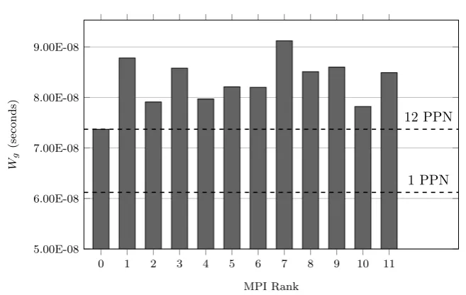
4.1 Comparison ofifluxWgvalues for 1 and 12 PPN on a single node 64

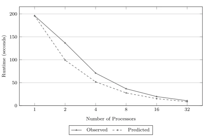
4.2 Comparison of recorded and predicted execution times for

single-level runs of the original HYDRA using 1 PPN . . . 67

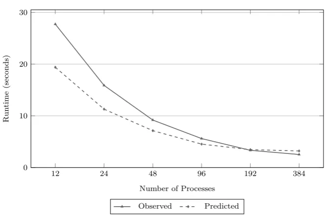
4.3 Comparison of recorded and predicted execution times for

single-level runs of the original HYDRA using 12 PPN . . . 68

4.4 Best-case performance behaviours for the OPlus communication

routines on two processors . . . 69

4.5 Worst-case performance behaviours for the OPlus communication

routines on two processors . . . 70

4.6 Compute/communication/synchronisation breakdown for the

orig-inal and optimised HYDRA, as: (a) time in seconds; and (b)

percentage of execution time . . . 71

4.7 Comparison of observed and predicted execution times for

single-level runs of the optimised HYDRA, using 1 PPN . . . 73

single-level runs of the optimised HYDRA, using 12 PPN . . . 74

multi-grid runs of the optimised HYDRA using 1 PPN . . . 77

multi-grid runs of the optimised HYDRA using 12 PPN . . . 78

5.1 Trace of solver iteration events (ncycles = 3) . . . 86

5.2 Comparison of actual and predicted compute time (Rotor37, 8

million nodes; geometric partitioning; Tinis) . . . 91

5.3 Predicted compute time percentage error (Rotor37, 8 million

(17)

5.4 Comparison of actual and predicted runtime (Rotor37, 8 million

nodes; geometric partitioning; Tinis). See Table 5.2 for

confi-dence intervals. . . 93

5.5 Total predicted time percentage error (Rotor38, 8 million nodes;

geometric partitioning; Tinis). . . 94

5.6 Comparison of HYDRA’s actual and predicted runtime (Rotor37,

8 million nodes, ParMETIS; Tinis) See Table 5.2 for confidence

intervals. . . 96

5.7 Percentage error for model costs (Rotor37, 8 million nodes, ParMETIS;

Tinis) See Table 5.2 for confidence intervals. . . 97

5.8 Percentage error ofWgcalculation techniques for max edge

com-pute (Tinis) . . . 98

5.9 Impact of partitioning data source on model (Tinis) . . . 100

5.10 Predicted effect of partitioning algorithm on HYDRA’s runtime

and the speedup from using ParMETIS over a geometric

parti-tioning . . . 102

6.1 Comparison between the runtime and parallel efficiency of

Compact-and Mini-HYDRA for each level of the multigrid . . . 112

6.2 Comparison between Mini- and Compact-HYDRA in terms of

the correlation of PAPI counters with parallel inefficiency . . . . 114

6.3 Comparison between OpenMP strong scaling behaviour between

Intel Ivybridge and Intel Haswell for both Compact- and

Mini-HYDRA . . . 117

6.4 Impact of using the Intel Fused Multiply-* instructions with and

without auto-vectorisation on both Compact- and Mini-HYDRA 118

6.5 Performance impact of using auto-vectorisation on both

(18)

List of Tables

3.1 Hardware/software configuration of Napier . . . 48

3.2 Hardware/software configuration of Power8 . . . 48

3.3 Hardware/software configuration of ARCHER . . . 49

3.4 Hardware/software configuration of Minerva . . . 49

3.5 Hardware/software configuration of Tinis . . . 50

3.6 Mapping between loop names and the identifiers assigned by the auto-instrumentation tool . . . 54

3.7 Confidence intervals for HYDRA’s runtime on Power8 at different Simultaneous Multithreading (SMT) levels . . . 56

3.8 Confidence intervals for HYDRA’s Runtime on Napier . . . 57

4.1 Description of compute and communication model terms for a single-level HYDRA run . . . 63

4.2 Confidence intervals for HYDRA’s runtime on Minerva when us-ing the LA Cascade dataset . . . 68

4.3 Description of additional model terms required to support multi-grid HYDRA runs . . . 75

4.4 Confidence intervals for HYDRA’s runtime on Minerva when us-ing the Rotor37 dataset . . . 76

4.5 Model validation for multigrid runs of HYDRA on the LA Cas-cade dataset (Confidence intervals are in Tables 4.2 and 4.4) . . . 79

4.6 Model validation for multigrid runs of HYDRA on the Rotor37 dataset . . . 82

(19)

5.2 Confidence intervals for HYDRA’s runtime on Tinis when using

either a Geometric Partitioning or ParMETIS to partition the

input deck. . . 95

6.1 Confidence intervals for Compact- and Mini-HYDRA’s runtime

on Tinis . . . 113

6.2 Confidence intervals for Compact- and Mini-HYDRA’s runtime

(20)

Listings

3.1 Pseudo-code for HYDRA’s smooth loop . . . 41

3.2 Code-snippet fromvflux, a typical OPlus parallel loop . . . 44

3.3 An example auto-instrumentation rule which matches the entry

to an OPlus parallel loop, and action, to insert timers and gather

the set name associated with this loop . . . 52

6.1 Pseudo-code skeleton of the mini-application . . . 108

(21)

CHAPTER

1

Introduction

Simulation is an important cornerstone of scientific experimentation and has

found widespread use in a variety of domains including engineering, physics and

economics. This is because simulations can be constructed to represent

environ-ments that would be prohibitively expensive, impossible or simply against the

law to physically create. Additionally, simulations can allow the measurement

of variables which would be challenging to record in practice. Furthermore,

simulation techniques are able to emulate processes faster than they occur in

realtime, allowing the outcome of these processes to be predicted ahead of time.

While some scientific simulations can be run on a computer which might be

found under an office desk, achieving the level of detail required for state of the

art applications in a time frame where the results are still of value, typically

requires execution on large parallel computers.

These parallel computers are housed not under desks, but in dedicated

facil-ities with their own cooling and power systems, and the most powerful are

sev-eral orders of magnitude more performant than any desktop computer. Floating

Point Operations per Second (FLOP/s) are one standard metric for quantifying

the performance of parallel computers – this metric indicates how many

calcula-tions (e.g. addition, multiplication) can be performed on floating point numbers

per second. The TOP500 list has been tracking the computing power available

on the fastest 500 computers from the last decade; from this it can been seen

that the computational power of machines has been increasing exponentially

since recording started in 1994, to the point where the most performant of these

machines can perform 93 petaFLOP/s (1015 FLOP/s) [118]. This regular

(22)

greater capacity and capability.

The scientific simulations which run on these machines are the product of

years of research and are invaluable for their respective use cases, therefore

keeping them functioning on modern hardware is of paramount importance.

However, while hardware has progressed rapidly over the last four decades,

these simulations have largely remained unchanged and are often still written

using the programming languages around at the time of their inception. This,

along with their size makes adding new features, moving the applications to

up-coming parallel architectures, and running with larger degrees of parallelism a

significant time investment. It is therefore necessary to further the development

of performance engineering techniques, such as performance modelling (models

which allow reasoning about performance) and mini-applications (distilled

ver-sions of larger codes which are more tractable to experiment with) to aid with

overcoming these challenges.

This thesis represents over three years of performance engineering work on

HYDRA, a geometric multigrid, unstructured mesh code developed by

Rolls-Royce. HYDRA exemplifies the aforementioned challenges; it has existed through

over four decades of advances in parallel hardware and supporting tool chains;

it is written in FORTRAN77; and, it is tens of thousands of lines of code in size.

This work sees the construction of a runtime performance model of HYDRA,

which has primarily been used to i) validate HYDRA’s performance on several

machines at supercomputing centres around the United Kingdom, and ii) to

assess the continued suitability of competing partitioning algorithms.

Addition-ally this work presents the development of a mini-application; a smaller code

capturing only HYDRA’s primary computational behaviours. This is used to

assess the impact of the hardware features available from the next generation

(23)

1,975 1,980 1,985 1,990 1,995 2,000 2,005 2,010 2,015 10−1

100

101

102

103 104

105

106

107

108

Year

P

erformance

[image:23.595.128.436.123.385.2]

(GFLOP/second)

Figure 1.1: Visualisation of top supercomputer performance over time (uses data from [118, 145])

1.1 Motivation

Since the introduction of the TOP500 list [118] in 1994, the performance of the

world’s fastest computers has been increasing exponentially, from just under

100 gigaFLOP/s (109_{) to almost 100 petaFLOP/s in 2016 (see 1994 to 2016 in}

Figure 1.1). Up until 2006, this increase in performance was primarily enabled

by increases in transistor densities, which was predicted to double every 18-24

months [120]. These performance increases were courtesy of Dennard scaling: as

the size of a transistor is reduced, power consumption is also reduced meaning

that a chip with double the density of transistors, can operate using the same

power as one with half the density (but the same area) [43]. Additionally,

shrinking transistors also reduces the switching delay which results in higher

clock speeds [51]. What this meant for the custodians of scientific simulations, is

that a reduction in time to solution could be expected every time new hardware

(24)

However, post 2006 Dennard scaling began to breakdown due to physical

limits being reached (e.g. size of the transistor). This caused CPU designers

to shift their attention to optimising the execution architecture to maximize

the amount of instructions per cycle. This has resulted in a transition to using

CPUs with multiple execution cores, which allows the CPU to run at a lower

clock speed while being able to process the same number of instructions. In

ad-dition to this, the execution cores have become more complex with many more

opportunities for exploiting parallelism such as wide vector units and

Simul-taneous Multithreading (SMT). Further to this, the recent trend has been to

use many-core architectures, which trade a few complex cores for many simple

cores. Unfortunately, performance increases from these architectural changes

are not free; therefore application developers must actively invest time

perfor-mance engineering their application to take advantage of them [146].

These, and future architectural shifts, coupled with the fact that many

scien-tific simulations were originally written for the vector machines of the 1970s (see

1977 in Figure 1.1), has made it increasingly difficult to continuously evaluate

and prepare a code for performant future use. Many High Performance

Comput-ing (HPC) centres are therefore turnComput-ing to performance engineerComput-ing tools and

methodologies, such as predictive performance modelling and mini-applications

to facilitate system evaluation, to aid in the comparison of multiple candidate

machines, to investigate optimisation strategies, and to act as a vehicle for

port-ing codes to novel architectures. This thesis focuses on the application of

in-strumentation, the extension of runtime performance modelling techniques and

mini-applications (a relatively new form of performance engineering) to support

the shift of large, legacy, unstructured mesh, geometric multigrid applications

(25)

1.2 Problem Statement

This thesis builds upon both the performance engineering techniques of

run-time performance modelling and mini-applications in the context of

unstruc-tured mesh, geometric multigrid codes; applications which represent their input

geometries at varying resolution. An unstructured mesh can be represented as

a graph (G = (V, E)), where V is a set of nodes and E ={(a ∈ V, b ∈ V)}

is a set of edges, which are arbitrary pairs of nodes. The class of simulation

which is examined by this thesis, performs computation by iterating overEand

accessing the nodes aand b as defined by the pair. Further to this, geometric

multigrid applications operate on a list of these graphsM = [G0, ..., Gn], where

the results of computation over the edges of one graph of propagated to the

others. In this thesis the aim is to overcome some of the challenges associated

with performance engineering this class of code.

Theaand b of any edge in any G are accessed indirectly (i.e. through the

edges) and are unlikely to be contiguous in memory; this posses a challenge to

computers which rely on this to achieve consistent performance. This

uncer-tainly in performance is a barrier predicting the runtime of computations over

edges, as the processing time of each edge can vary. This thesis aims to quantify

the impact of this uncertainty on model accuracy and propose a solution.

Unstructured meshes pose an additional challenge to modelling when

at-tempting predict runtime at large scale. This is because selecting an optimal

partitioning of a graph is an NP-Hard problem, and the generation of these

partitions must be performed by a partitioning algorithm to approximate the

solution [20]. This means that in order to obtain a representative partitioning

for a particular scale of execution, a partitioner must first be run at that scale.

This severely limits the predictive power of any performance model of

unstruc-tured mesh codes. This thesis aims to develop methods to gather representative

partitioning data which can be used by performance models of unstructured

(26)

The development and validation of mini-applications is a challenging

pro-cess, as it is not well defined in the literature and differs depending on the

intended use case of the application. This thesis contributes to this gap, by

de-tailing the experience of developing, validating and using a geometric multigrid,

unstructured mesh mini-application.

The research presented in this thesis is performed as part of a project to

support the continued development of HYDRA, a geometric multigrid,

unstruc-tured mesh code developed by Rolls-Royce. This code has been developed over

the last four decades and as such it contains a vast amount of company

knowl-edge. This thesis demonstrates the impact of the developed tools, performance

model and mini-application by aiding Rolls-Royce with the continuing challenge

of moving HYDRA onto machines with more modern architectures and larger

degrees of parallelism.

1.3 Contributions

Specifically, this thesis and its products make the following contributions:

• The development of an automatic instrumentation process is presented

which allows for unprecedented flexibility in terms of implementation

lan-guage, the language to be instrumented and the instrumentation to be

in-serted. This process is implemented and then demonstrated by applying a

common set of instrumentation to three different variants of HYDRA: two

being chronological releases and the third being optimised to reduce

syn-chronisation costs. The data from which is then used to compare historical

changes in performance and to quantify the impact of the optimisation.

In work that is not presented in this thesis, the auto-instrumentation tool

has been used in support of collecting performance data from HYDRA

on a variety of platforms, such as Intel Haswell/Ivybridge, IBM Power 8,

BlueGene/Q so that their potential may be compared. It is expected that

(27)

in the future;

• The development of a runtime performance model of an unstructured mesh

code is detailed, which is able to capture the expected scaling behaviour of

HYDRA, and its proprietary communications library, the Oxford Parallel

Library for Unstructured Solvers (OPlus), when running on a grid with

one level. Through the introduction of a small number of additional model

terms, this model is generalised to multigrid simulations. The simple

re-lationship between these two models significantly reduces the complexity

of benchmarking a new platform, as it enables the extrapolation of

com-plete production runtimes using data collected from the execution of small

single-level datasets. The use of the performance model is demonstrated

by identifying a synchronisation issue which degrades performance by up

to 29.22% on machine configurations that exhibit poor support for

over-lapping computation with communication. An optimisation is then

ap-plied which decreases the cost of communication and synchronisation by

3.01×and total runtime by up to 1.41×. That it is possible to accelerate

HYDRA to such a degree demonstrates both the accuracy of the model

and the importance of reassessing whether an application’s original design

assumptions still hold on new hardware/software configurations. Given

this accuracy, the model has been put into use by Rolls-Royce to confirm

the correct strong scaling behaviour of HYDRA on small-scale evaluation

hardware;

• The analytical runtime model for multigrid applications is further

gen-eralised to support multiple cycle types (e.g. V-Cycle, W-Cycle) and a

variable number of time steps per iteration. Additional details are

incor-porated in to the performance model: buffer pack/unpack costs, runtime

costs from all 300+ loops in the code base, and performance

informa-tion for different memory access patterns. These addiinforma-tional details are

(28)

geometric partitioning algorithm and ParMETIS to partition the NASA

Rotor37 input deck, with a maximum absolute error of 12.63% and 11.55%

respectively. Additionally, the performance model’s accuracy is reported

on 1,008 cores of an Ivybridge-based cluster (ARCHER). These additions

to the model allow a wider range of workloads to be successfully modelled;

• Moses, an unstructured domain decomposition mini-application, is

devel-oped which is able to convert partitioning data from multiple

algorithm-s/libraries (ParMETIS, METIS, Scotch) at varying scale (up to 100,000

partitions) for use with the runtime performance model. This data allows

predictions to be made at scale without first running HYDRA at scale to

collect set sizes. Runtime predictions made using this data have an error

in runtime of at most 7.31% over 512 processes, when compared against

predictions made with empirically collected partitioning data. The use

of Moses is demonstrated in conjunction with the runtime performance

model to predictively compare the relative effect on HYDRA’s runtime of

using Scotch, ParMETIS, METIS and a geometric partitioning algorithm

on up to 30,000 cores. Using the runtime model in conjunction with Moses,

predicts that the geometric partitioning algorithm will cause reduced

per-formance in HYDRA at 512 processes when compared to ParMETIS;

• Finally, a mini-application is introduced which operates on datasets with

the following properties: i) unstructured mesh, ii) geometric multigrid,

and iii) a variable number of neighbours per node. It is validated

us-ing two previously developed techniques which have not previously been

applied to this class of code. These techniques provide evidence of the

sim-ilarity between the mini-application and the parent code in terms of their

shared memory scalability. To conclude, the use of the mini-application

is demonstrated by quantifying the impact of the new hardware features

introduced to the Intel Haswell platform over Intel Ivybridge for geometric

(29)

instruc-tions and the AVX2 features have a limited impact on performance, but

there is potential for Intel Haswell to deliver application results at a much

lower total energy. At the time of writing this thesis, this mini-application

is being used as part of procurement exercises, and it is hoped that this

mini-application will be used in the future as a vehicle for optimisation,

porting and execution on machines where HYDRA is not cleared for use.

1.4 Thesis Overview

The remainder of this thesis is structured as follows:

Chapter 2 contains knowledge of parallel computing essential to

understand-ing the field: the lexical set, the opportunities for parallelism provided by

the hardware, and the software which enables the usages of this hardware.

This chapter continues by providing historical background to performance

engineering techniques (the primary focus of this research) up to state of

the art techniques and their relative merits and shortcomings.

Chapter 3 introduces the context for this research – unstructured mesh,

ge-ometric multigrid applications, specifically Rolls-Royce HYDRA, an

in-stance of this class of code. The features and structure, and their

associ-ated performance challenges, of these codes and those specific to HYDRA

are described. This introduction also details the challenges associated

with collecting data from HYDRA and other unstructured mesh

applica-tions and how these were overcome using newly developed instrumentation

tools. Finally this chapter presents performance information collected

us-ing these instrumentation tools, which serves as an overview of HYDRA’s

performance and a demonstration of the instrumentation tool’s flexibility.

Chapter 4 presents the initial development of a runtime performance model of

HYDRA, first for single level execution and then for multigrid execution.

(30)

cores. The value of this model is then demonstrated by identifying

detri-mental communication behaviours through a discrepancy in the predicted

(expected) and actual contribution to total runtime from synchronisation

costs.

Chapter 5 generalises the runtime performance model to support a variable

number of time steps per iteration, arbitrary multigrid cycle types and

all datasets which rely solely on loops. This chapter then identifies the

challenge of generating representative partitioning data for use in large

scale runtime predictions, to which the construction of a partitioning

mini-application is presented as a solution. The use of this mini-mini-application is

demonstrated by performing a predictive evaluation of the effect various

partitioning libraries have on application runtime.

Chapter 6 details the construction, validation and use of mini-HYDRA, a

mini-application designed to compliment the performance model

devel-oped in previous chapters. The mini-application is used to quantify the

impact the new instructions introduced as part of Intel Haswell (Fused

Multiply-Add (FMA) and AVX2) on HYDRA’s inviscid flux kernel.

Chapter 7 concludes this thesis with a summary of the work carried out and a

discussion of the impact this research has had on the individuals involved

in this project. Additionally the limitations of this work and possible

future research directions to either rectify these limitations or broaden

(31)

CHAPTER

2

Parallel Computing and Performance Engineering

Parallel computing was born from the need to run algorithms of i) increasing

complexity to completion in a time frame such that the result is still of value,

and ii) over increasingly larger input domains. As the name suggests, parallel

computing enables this by running the independent computational parts of an

algorithm simultaneously (in parallel), as apposed to performing calculations

one by one (serially). One classical example of this involved human computers,

rather than the electronic computers available today, who performed engineering

calculations at the Langley Memorial Aeronautical Laboratory in the 1940s [31].

Groups of human computers existed at this laboratory in order to field these

calculations in parallel, and in some cases if a group reached capacity, the

cal-culations were sent to a secondary group.

The purpose of this chapter is to present the foundation of knowledge which

the work in this thesis builds upon. Not only does this foundation give the

thesis context, it also details the lexicon and concepts which are used

through-out. Specifically, this foundation consists of i) a description of the physical

hardware and software which comprise the domain of High Performance

Com-puting (HPC); ii) the laws and abstract models which capture the behaviour of

HPC applications; and, iii) an introduction to modelling and benchmarking the

performance of HPC applications and the relative merits of these techniques.

2.1 The Composition of a Parallel Machine

Today’s parallel computers often consist of electrical circuits, fibre interconnects

and large cooling apparatus. These electrical computers allow many

(32)

Parallel Machine

Compute Node (1)

CPU (1)

Core (1) Core (n)

Accelerator (1)

CPU (n) _…

…

Core (1) … Core (n)

…

… Accelerator_(n)

Compute Node (n)

CPU (1)

Core (1) Core (n)

Accelerator (1) CPU (n)

…

Core (1) … Core (n)

…

[image:32.595.156.437.135.340.2]

… Accelerator_(n)

Figure 2.1: An abstract representation of a parallel machine configuration

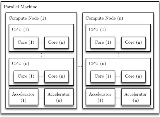
will be exploited in order to achieve maximum benefit [144]. Opportunities for

parallelism are exposed throughout all the hardware components of a parallel

machine (see Figure 2.1) from the bit-level in a single Central Processing Unit

(CPU) core, to the data-level where datasets are partitioned across groups of

compute nodes.

2.1.1 Core

Bit-level parallelism allows the CPU core (see Figure 2.1) to push more bits

around per clock cycle, typically by increasing the size of the registers.

Histori-cally, this increase in bits has moved from 4 up to 64 bits [38]. As an example

of how this change can improve performance consider a CPU core which

oper-ates on 32-bit registers and needs to perform an operation on 64-bit numbers –

it must perform the calculation in two parts, thereby taking two clock cycles.

However, a CPU capable of operating on 64-bit registers is able to complete the

same calculation in a single clock cycle.

At a slightly higher level of parallelism in the CPU core, there is Instruction

(33)

which allow data independent instructions to progress through the CPU core in

parallel. ILP is achieved through a variety of mechanisms in order to maximise

the use of the CPU core under a variety of workloads. The first ILP mechanism

to mention is pipelining; this involves separating the handling of instructions

into distinct stages, with separate hardware for each [148]. The most basic

pipeline has separate fetch, decode and execute units. This decomposition allows

the decoding of an instruction to occur in parallel with the fetch of the next

instruction.

Further parallelisation can occur at each of the stages in the pipeline by

duplicating and providing specialised execution units – this is known as a

su-perscalar architecture [148]. An example of this is the Intel Haswell CPU core

which, has two execution units capable of performing an Fused Multiply-Add

(FMA) instruction. In order to maximise the use of these additional execution

units, techniques are employed such as dynamic [87] and speculative

execu-tion [148]. The combinaexecu-tion of these techniques allows the CPU core to begin

two FMA operations simultaneously [103] and would benefit the computation

defined by Equation 2.1 as the partial resultsaandehave no data dependencies

and can therefore be performed simultaneously.

a=b∗c+d;

e=f∗g+h;

r=a+e;

(2.1)

In the case of the decoder, not only can they fetch and decode multiple

instructions simultaneously, they can also employ macro-fusion to exploit

paral-lelism at the micro-operation level (the sub-operations which form instructions).

This is achieved by fusing the micro-operations from different instructions into

a single, but more complex micro-operation [62]. Given a decoding unit which

(34)

of macro-fusion can increase the number of decodes from four to five per cycle,

thereby reducing the pressure on this unit.

Another opportunity for parallelism in the CPU core is provided by the

pres-ence of vector units. These enable data level parallelism by handling dispatched

vector instructions that apply the same operation to several data items in

paral-lel [38]. One such example of a vector instruction isvaddpd, which adds two sets

of 64-bit doubles [90]. The number of operations these instructions perform in

parallel depends on the width of the registers they use. While in the past, vector

lengths were large [145], the trend at the time of writing this thesis is for CPU

cores to have vector lengths of four or eight 64-bit doubles [89]. In addition to

enabling arithmetic in parallel, vector instructions exist to push data, such as

thevmovapdinstruction, which moves packed and aligned 64-bit floating point

values [90].

Parallelism is not limited to arithmetic operations; there are also

oppor-tunities in the CPU core for Memory Level Parallelism (MLP) [148]. This

mechanism allows multiple memory operations to occur simultaneously or

over-lap. CPU cores with MLP often exploit this by prefetching data elements from

slower to faster access memory before the data is required by an instruction,

in the hope it will decrease cache misses and increase achieved memory

band-width. MLP is important as it helps maximize the use of the available memory

bandwidth, which can be a bottleneck for performance [165, 167]. Essentially,

as a higher percentage of an application’s arithmetic is parallelised, the more

memory bandwidth is required to feed the calculations until this becomes the

bottleneck.

2.1.2 CPU

At the next level of the hardware hierarchy (Figure 2.1) there is Symmetric

Multiprocessing (SMP), a configuration consisting of multiple CPU cores. This

configuration is capable of exposing thread and task level parallelism [131] by

(35)

detailed in Section 2.1.1. At the most basic level, a CPU core offers Simultaneous

Multithreading (SMT) (multiple threads of execution per core) to increase the

use of a superscalar architecture, by increasing the sources of instructions [131]

e.g. Intel Hyperthreading [153]. At the other end of the spectrum there are

SMP systems with multiple CPUs, each with multiple cores, which can in turn

support multiple threads of execution. At this point, it becomes important to

consider the arrangement of these components as this impacts the efficiency of

communicating data between them.

There are two classes of SMP system: Non-uniform Memory Access (NUMA)

and Uniform Memory Access (UMA). In an UMA system, CPU cores can access

their local shared memory at the same latency and bandwidth as the shared

memory located on other cores. In a NUMA system CPU cores can access

their local memory faster than the local memory of other CPU cores [131].

The configuration shown in Figure 2.1 gives rise to two CPU NUMA regions:

communication between cores on the same CPU and between cores on different

CPUs. Due to the difference in communication time between NUMA regions,

locating data close to the CPU core which is operating on it can make a huge

difference to performance [15, 168]. Typically parallel machines use NUMA due

to its favourable memory size scaling over UMA [131].

2.1.3 Accelerators

The inclusion of accelerator cards in parallel machines has become increasingly

popular in recent years and in fact two of current top three in the TOP500 list

(Tianhe-2 and Titan) feature them (using Intel Xeon Phis and Nvidia Teslas

respectively) [118]. This increase in popularity is due to the potential of

ac-celerator cards to deliver power efficient computations [133], in an attempt to

overcome one of the challenges in HPC as outlined by the Department of Energy

(DoE) [76].

The basic concept behind the Graphics Processing Unit (GPU) and the

(36)

amount of fine-grained parallelism to computing applications. This is in

con-trast to a CPU which contains fewer general purpose cores. In the case of the

Intel Xeon Phi (Knights Corner) it has 61 cores, whereas an equivalent CPU,

the Intel Xeon E5-2670 has 8 [75]. The trade-off is that the cores on the Intel

Xeon Phi are simpler (e.g. they use in-order execution) and are lower clocked

compared to their CPU counterparts. The strength of the simpler cores is that

they have a larger degree of SMT, longer vector registers, they are greater in

number and have increased memory bandwidth [75]. The potential for

individ-ual applications to benefit from this configuration is usindivid-ually non-obvious and

must be assessed by way of an in-depth performance study on a per accelerator

basis.

2.1.4 Compute Node

At the final level of the hardware hierarchy (see Figure 2.1) there are

multi-ple connected physical machines, each containing multimulti-ple CPUs thus further

scaling the capacity for thread and task level parallelism. This configuration is

known as a distributed memory system [131].

As with the CPU level of the hierarchy, it is important to consider the

ar-rangement of the components (compute nodes) and additionally the medium by

which they are connected as this impacts performance [131]. Another

consider-ation is the method by which a problem is partitioned between the distributed

memory as this influences factors such as idle time due to load imbalance and

time spent communicating data.

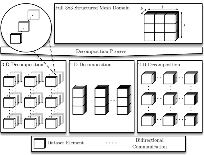
2.2 Parallel Data Decompositions

Many HPC applications simulate physical processes such as heat transfer and

fluid flow; examples of such applications include LAMMPS [137], a molecular

dynamics simulation, and OpenFOAM [92], a fluid dynamics simulation.

(37)

3-D Decomposition

Full 3x3 Structured Mesh Domain

1-D Decomposition 2-D Decomposition

Dataset Element _{Communication}Bidirectional Decomposition Process

i

[image:37.595.135.462.134.382.2]

j k

Figure 2.2: 1-, 2- and 3-D structured mesh decompositions

mesh which must be partitioned between compute nodes prior to execution on a

distributed memory machine (Section 2.1.4). The process used for partitioning

can impact performance because it influences both the ratio of computation to

communication and the quality of the load balancing. Furthermore, the

selec-tion of partiselec-tioning process depends on whether it is to be used on a structured

or unstructured mesh.

2.2.1 Structured Mesh

A structured mesh is a regular arrangement of points with a topology that is

apparent from their position in space. An example demonstrating this is given in

the top pane of Figure 2.2, where the quantities of the simulation are represented

as averages over each sub-cuboid.

Decomposing a structured mesh is achieved using either a 1-, 2- or 3-D

de-composition, as visualised by the lower set of three panes in Figure 2.2. The

(38)

num-u

j k

b

a

f

v i

Mesh Node

Edge Partition Boundary

Figure 2.3: Partitioning an unstructured mesh

ber of threads available. Each of these decompositions achieves a perfect load

balance, although in practice this only occurs when the number of processors

is an exact divider of one of the domains sides (i, j or k), a square number

or a cubic number, in the case of 1-, 2- and 3-D decompositions respectively.

However, the ratio of communication to computation does change depending

on the chosen decomposition, with a 3-D decomposition theoretically being the

most favourable [105].

2.2.2 Unstructured Mesh

An unstructured mesh (see Figure 2.3) is a collection of nodes (e.g. j and u),

edges (e.g. betweenuandv) and faces (f), with the nodes being at an arbitrary

position in space. The flexibility of the unstructured mesh allows complex

ge-ometries to be represented and the simulation resolution can be increased (and

also the computation time) only in regions of importance by altering the density

of mesh points [114].

The neighbours of a node in an unstructured mesh are not implicitly defined,

(39)

using offsets to the array indices. This means that an explicit list of neighbours

must be maintained, so that when computation over nodes is performed (e.g. the

accumulation of fluxes) data can be read from the required locations. This has

implications for the spacial and temporal locality of accesses when gathering

unstructured mesh features from memory, as a mesh node’s neighbours can

appear at arbitrary strides either side of its memory location.

Unlike a structured mesh, which can often be divided using algebra, an

unstructured mesh must be load balanced between distributed memory

loca-tions using specialised algorithms which are the result of numerous bodies of

research [63, 97, 128, 152, 164]. These algorithms are necessary to partition

unstructured meshes because it is not immediately clear how the mesh should

be divided, due to the arbitrary position and the number of neighbours of its

nodes. For example in Figure 2.3, mesh nodesuandbare in partition zero and

mesh nodesv,aandiare in the first partition, with a total of two edges cut on

level zero. However, some other arbitrary line could be drawn to partition the

mesh nodes.

Ideally both the number of edges cut and the load imbalance between the

number of nodes in each partition should be minimised, as a high value of the

former means increased communication time, and an high value of the latter

results in increased processor idle time. Finding an optimal partition is

NP-Hard and therefore these algorithms serve to find approximations to the optimal

solution [20].

2.3 Parallel Programming Laws and Models

When running and developing HPC applications it is only natural to want to

quantify their performance (e.g. time to results, use of parallelism). This

sec-tion covers the most basic performance metrics and laws which govern their

(40)

2.3.1 Speedup

S(n) = Ra Rb

(2.2)

Speedup (S(n) in Equation 2.2) is the ratio of two performance values,Ra and

Rb, wherenis the variant between these values [131]. TypicallyRa andRb are

application runtimes from either, two different variants of the same application,

or the same variant run using different degrees of thread level parallelism. In

the latter case, n would be the number of threads Rb was executed with. As

an example, consider an application that can exploit thread level parallelism

which has had its runtime recorded using both a single thread and four threads.

Applying Equation 2.2 to these runtimes, with Ra being the single threaded

runtime andRb being the runtime when using four threads, will yield the value

S(4) which indicates how many times faster (or slower) the multi-threaded

ex-ecution was compared to the serial run. While this is a useful summary metric,

especially when comparing the effectiveness of different code optimisations (e.g.

with and without using vector units) care must be taken when reporting speedup

in the case where multiple code optimisations have been applied, as it becomes

unclear which optimisation the speedup came from.

2.3.2 Parallel Efficiency

Pe(n) =

S(n)

n (2.3)

Parallel efficiency (Pe(n) in Equation 2.3) codifies the extent to which an

ap-plication utilises opportunities for parallelism as opportunities are increased

(n) [131]. Equation 2.3 has speedup as one of its constituents. This captures

the performance change when using different degrees of thread level parallelism.

This speedup value is normalised by the degree of thread level parallelism used

as this is the speedup expected from an application which fully uses the available

(41)

0 ₂1 ₂3 ₂5 ₂7 ₂9 ₂11 ₂13 ₂15

0 21

23

25

27

29

Number of Processes

Sp

eedup

Both lawsfp = 1.0 Amdahl’s Lawfp = 0.99

Amdahl’s Lawfp= 0.95 Gustafson’s Lawfp= 0.5

[image:41.595.127.438.122.393.2]

Gustafson’s Lawfp= 0.3

Figure 2.4: Amdahl’s Law and Gustafson’s Law for varying values of fp

applications, or quantify whether the cost of additional resources required to

make additional parallelism available to the application is worth the increase in

performance.

2.3.3 Amdahl’s Law

St(s) =

1 fs+fp_s

!

, St(s)≤

1 fs

(2.4)

While the metrics of speedup (S(n)) and parallel efficiency (Se(n)) capture

ob-served performance, neither attempt to bound performance, whereas Amdahl’s

law [6] (Equation 2.4) can provide an upper bound on speedup. It does this for

an entire application run (St) in terms of the fraction of parallel code (fp) and

serial code (fs), by pushing the speedup of the parallel region (s) to infinity. By

priming Equation 2.4 with various fractions (fpequal to 1.0, 0.99 and 0.95), the

(42)

that given an application where all of the code can be parallelised, the

maxi-mum achievable speedup is linear in the number of threads. For example, with

a fixed work load a single thread must perform all the work, but two threads can

perform half of all the work simultaneously; this is known as strong scaling. It

should be noted that this bound on speedup is not strictly true, as super linear

speedups can be observed in practice due to the degree of available parallelism

not being the only factor influencing application performance; typically super

linear speedups are observed as a result of the decreasing data associated with

each thread fitting into successively smaller (but faster) levels of cache.

Equa-tion 2.4 further indicates that for a given fracEqua-tion of parallel code, the runtime

will approach the runtime of the serial region as the degree of parallelism tends

to infinity. Even by having a serial region of 1% vastly impacts the overall

parallel efficiency of the application.

2.3.4 Gustafson’s Law

St(s) =fs+s(1−fs) (2.5)

Gustafson’s law [69] considers the bound on speedup for an entire application

(St) from a different perspective. Gustafson argued that in practice strong

scaling was not the norm, and that the problem size increased with increasing

degrees of parallelism (weak scaling); this behavior is codified in Equation 2.5

and plotted for varying proportions of parallel code in Figure 2.4. From this

figure it can be seen that even at much lower proportions of parallel code (fp

equal to 0.3 and 0.5), the predicted bound on speedup is much more optimistic

than the bound predicted by Amdahl’s law for considerably higher proportions

(43)

Requirements and Specification

Hardware Cycle Software Cycle

System Design

Tuning

Mid-life Upgrade Protoyping

Implementation

Installation and Acceptance

Requirements and Specification

Code Updates Implementation

Design

Optimisation Performance

Analysis Porting to System Codesign

[image:43.595.147.447.138.456.2]

Feedback

Figure 2.5: Hardware and software life cycle (adapted from [11])

2.4 Performance Engineering

HPC applications are complex pieces of software which are often tens of

thou-sands of lines of code long, developed over several decades, and are run with

hundreds of thousands of degrees of parallelism. These codes are of high utility

and therefore it is important to continually assess and improve their

perfor-mance on current hardware through optimisation and code updates, and also

prepare for future hardware (see Figure 2.5).

The hardware upon which HPC applications are run is just as complex as

the applications themselves, so it is also important to continually assess the

(44)

is necessary to replace it (see Figure 2.5). At this time is essential to have a tool

box of methods which allow the comparison of candidate replacement hardware

at the lowest level of parallelism, to indicate how well a particular application

will perform on a new architecture and/or use finer grained parallelism, and can

validate the performance of an application on new hardware.

Performance engineering is a field which encompasses many mature

tech-niques (e.g. benchmarking, mini- and compact applications, profiling and

ana-lytical performance modelling) developed to support each stage of this complex

cycle of developing and maintaining HPC systems and applications.

2.4.1 Profiling and Instrumentation

Profiling an application is the act of extracting performance data from a

run-ning application. Examples of data which can be collected about an application

include: the time duration and frequency of code blocks (e.g. gprof [68]), cache

hits and number of floating point operations (e.g. Performance Application

Pro-gramming Interface (PAPI) [18]), power draw (e.g. RAPL [39]) and memory

usage (e.g. Valgrind massif [129]). These metrics can be used to identify targets

for optimisation and parallelisation. For example, a routine which uses memory

inefficiently may demonstrate a high memory watermark or a high cache miss

rate, and a routine which would benefit the most from parallelisation efforts

would dominate runtime.

There are two main classes of profiling: statistical and tracing. Statistical

profiling periodically samples performance values whereas tracing collects all

data relating to a particular value (e.g. gprof [68]). This means that while the

statistical profiler collects incomplete data, and may even overlook performance

values entirely, it has the potential to exhibit lower overhead when running

at scale than a tracer (e.g. Sun Studio [91]). In the case of determining the

frequency and duration of code regions, a statistical profiler will periodically

sample data at the position of execution and then compile these samples in to

(45)

regions.

Another consideration to take into account is the method of instrumentation

by which values are collected. There are three main approaches to

instrumen-tation (as mentioned by Chittimalli and Shah [33]), these are binary, byte code

and source code instrumentation. The use of byte code instrumentation is

im-mediately ignored, as it applies to code running in a virtual machine, which

does not apply to the codes in this thesis. Source code based instrumentation

requires the augmentation of an applications source code, which can happen

before (e.g. PAPI [18]) or during compilation (e.g. gprof [68]). Static binary

instrumentation (e.g. Dyninst [160]) augments the compiled binary, naturally

this technique does not require the code to be recompiled. Similarly, dynamic

binary instrumentation (Intel PIN [106] and Valgrind [129]) does not require a

recompilation but may introduce runtime overheads.

2.4.2 Benchmarks, Mini- and Compact-Applications

The comparison of hardware choice and software optimisation approaches is

an-other core part of performance engineering. To enable such comparisons a vast

number of benchmarks, mini- and compact applications have been developed.

Benchmarks are applications which exercise and subsequently quantify the

per-formance of a particular subsystem, or group of subsystems belonging to a

par-allel machine, under a defined workload. Benchmarks come in a variety of forms.

At the lowest level, benchmarks can exercise and measure the performance of a

single subsystem (e.g. main memory [115], cache [121] and inter-compute node

interconnect [88]) and at the highest level, there are benchmarks which

cap-ture and asses the performance of common computational patterns, for example

Single-Precision AX Plus Y (SAXPY) [45, 122], or even the behavior of a specific

parent application (mini- and compact-applications) [110, 134, 140, 156].

There are several benchmarks which facilitate comparison of computational

power between different machines or single CPUs, but the most famous has to be

(46)

LINPACK benchmark solves dense systems of linear equations and is therefore

Floating Point Operations per Second (FLOP/s) heavy. While this makes it an

excellent compute benchmark, doubts about its usefulness have been raised as it

is only representative of a single class of code. This has led to the development

of further benchmarks [46, 47, 109]. Other compute benchmarks include the

Livermore Loops [54] and the Thirteen Dwarfs [7].

Power is another metric by which to compare machines and individual CPUs,

and is becoming an increasingly important concern. The FIRESTARTER

bench-mark can be used extract “near-peak power consumption” from a particular

CPU [70]. However, in the case of a machine comparison, the amount of useful

work done needs to be taken into consideration, meaning FLOP-per-Watt [53]

is a better method of comparing two architectures in terms of power.

As with the CPU, several benchmarks exist for characterising the different

levels of a memory system. For measuring the peak memory bandwidth from

main memory, the STREAM benchmark can be used [115]. This delivers result

in MB/s for four common memory access patterns: copy, scale, add and triad.

A second benchmark exists, Cachebench, for measuring the memory bandwidth

from individual levels of cache to the CPU [121]. Both of these benchmarks

can be used to compare the memory bandwidth of several candidate machines

and can give an indication of how well a code which is bottlenecked by memory

bandwidth will perform (Section 2.1.1).

Benchmarks also exist to quantify the performance of shared and distributed

memory computations. At the shared memory level there is OpenMP for which

there is a benchmark to measure the overhead from using various operations

such as loop iteration scheduling and synchronisation [8, 21, 22, 58]. On the

distributed memory side, benchmarks such as Intel MPI Benchmark (IMB) [88]

and SKaMPI [142, 143] collect bandwidth and latency figures for various

mes-sage sizes. These Mesmes-sage Passing Interface (MPI) benchmarks can be used to

compare different MPI implementations (e.g. MPICH2, Intel MPI, OpenMPI)

(47)

A more recent trend has been to develop so called mini-applications, which

capture a subset of the key performance characteristics (e.g. memory access

pat-terns) from a class of applications or a parent code. Numerous mini-applications

have been developed, some of which have been released as part of projects such

as the Mantevo Project [77] and the UK App Consortium [158].

Mini-applications from these repositories and other standalone mini-Mini-applications have

been used in a variety of contexts: i) exploring the suitability of new

archi-tectures for molecular dynamics codes [134], ii) examining the scalability of a

neutron transport application [156], iii) to aid the design an development of a

domain specific active library [140] and, iv) exploring different programming

models [110].

2.4.3 Modelling Parallel Computation

The formation of Amdahl’s law in 1967 was a just a starting point for the

development of further abstract and concrete models governing and describing

the performance of both parallel hardware and applications. While Amdahl’s

law contains just a few parameters to represent both the software (fraction of

parallel code) and the hardware (number of processors), newer models have

potentially hundreds, characterising compute, communication behaviour and

synchronisation behaviour. The increase in parameters allows more complex

hardware and software behaviours, but brings with it a decrease in tractability.

However, performance models still provide a useful platform from which to

perform analyses.

Parallel Random Access Machine (PRAM)

In 1978, PRAM was proposed as one of the first models of parallel computing.

It was developed due to the need for a framework with which to develop parallel

algorithms while avoiding the nuances of real hardware [56]. This model has the

follow constituent parts: an unbounded set of processors P =p0, p1, ... which

(48)

instructions; an unbounded global memory and processor local memory, both

ca-pable of storing non-negative integers; a set of input registerI0, I1, ..., In; a

pro-gram counter; a per processor accumulator, also capable of storing non-negative

integers; and, a finite program A comprising the aforementioned instructions.

Computation then proceeds as follows:

1. The input is placed in the input registers: one bit per Ik.

2. All memory is cleared and the length of the program (A) is placed into

the accumulator ofP0.

3. Instructions are then executed simultaneously by eachp∈P.

4. The FORK instruction can be used to spawn computation on an idle

pro-cessor.

5. Execution stops when either aHALTinstruction is executed byP0or a write

instruction is executed on the same global memory location simultaneously

by multiple processors.

There are several deficiencies with PRAM, the first of which is the lack of

cost associated with communication. This prevents the model from being an

accurate representation for NUMA machines which have multiple

communica-tion layers (core-to-core, socket-to-socket and node-to-node). This lack of cost

associated with communication time additionally prevents the scaling behaviour

of an application from being modelled when run at large scale, where

commu-nication costs can dominate.

Bulk Synchronous Parallel (BSP) Computation Model

BSP was developed in 1990 by Leslie Valiant with the same underlying goal as

PRAM [150, 161], to provide a model which allows researchers to independently

develop parallel algorithms and hardware. BSP overcomes the primary flaw

with PRAM: there was no cost parameter for communication events, which

Performance engineering unstructured mesh, geometric multigrid codes

warwick.ac.uk/lib-publications

A Thesis Submitted for the Degree of PhD at the University of Warwick

Permanent WRAP URL:

http://wrap.warwick.ac.uk/89503

Copyright and reuse:

This thesis is made available online and is protected by original copyright.

Please scroll down to view the document itself.

Please refer to the repository record for this item for information to help you to cite it.

Our policy information is available from the repository home page.

Performance Engineering Unstructured Mesh,

Geometric Multigrid Codes

Richard Arthur Bunt

Doctor of Philosophy

Department of Computer Science

Contents

Acknowledgements

Declarations

Sponsorship and Grants

Abstract

Abbreviations

List of Figures

List of Tables

Listings

CHAPTER

1

Introduction

1.1

Motivation

1.2

Problem Statement

1.3

Contributions

1.4

Thesis Overview

CHAPTER

2

Parallel Computing and Performance Engineering

2.1

The Composition of a Parallel Machine

2.1.1

Core

2.1.2

CPU

2.1.3

Accelerators

2.1.4

Compute Node

2.2

Parallel Data Decompositions

2.2.1

Structured Mesh

2.2.2

Unstructured Mesh

2.3

Parallel Programming Laws and Models

2.3.1

Speedup

2.3.2

Parallel Efficiency

2.3.3

Amdahl’s Law

2.3.4

Gustafson’s Law

2.4

Performance Engineering

2.4.1

Profiling and Instrumentation

2.4.2

Benchmarks, Mini- and Compact-Applications

2.4.3

Modelling Parallel Computation