Portfolio optimization based on divergence measures

Munich Personal RePEc Archive

Portfolio optimization based on

divergence measures

Chalabi, Yohan and Wuertz, Diethelm

November 2012

Online at

https://mpra.ub.uni-muenchen.de/43332/

Portfolio Optimization Based on Divergence

Measures

Yohan Chalabi

_{Diethelm Wuertz}

Institute for Theoretical Physics, ETH Zurich, Switzerland

Computational Science and Engineering, ETH Zurich, Switzerland

November 2012

A new portfolio selection framework is introduced where the investor seeks the allocation that is as close as possible to his “ideal” portfolio. To build such a portfolio selection framework, theφ-divergence measure from information theory is used. There are many advantages to using theφ-divergence measure. First, the allocation is made such that it is in agreement with the historical data set. Second, the divergence measure is a convex function, which enables the use of fast optimiza-tion algorithms. Third, the objective value of the minimum portfolio divergence measure provides an indication distance from the ideal portfolio. A statistical test can therefore be constructed from the value of the objective function. Fourth, with adequate choices of both the target distribution and the divergence measure, the objective function of theφ-portfolios reduces to the expected utility function.

Keywords Portfolio weights modeling ·Divergence measures ·Dual divergence·

Information theory·Minimax optimization problems

JEL Classification C12 ·C13·C43 ·C61·G11

∗_{Corresponding author. Email address: chalabi@phys.ethz.ch. Postal address: Institut für Theoretische Physik,}

1 Introduction

The portfolio selection problem consists of finding a repartitioning of a wealthW intoN financial instruments with allocation w_{= (w1, w2, . . . , wN)}T _{such that it produces a feasible portfolio}

that is most adequate for the investor. For an investor concerned with risk, the criterion of adequacy would be based on a portfolio pseudo-invariant transform,Y =TP(w, Vt, It), which

maps the portfolio selection, w_{, the instrument values, Vt, and the information known at}

t, It, to a random variate defined on the probability space (Ω,F,P), which models the risk

perception of the investors. This is a rather general formulation of the portfolio selection problem. A more pragmatic approach of the portfolio selection problem is the risk-reward paradigm, which originated in the Nobel-memorial-awarded mean-variance (MV) portfolio selection of Markowitz [1952]. It consists of finding the weights that produce the smallest variance of the financial returns under specific mean return constraints. The mean-variance paradigm is usually represented as the minimization of anyRisk measure (the variance, in the MV framework), with respect to aReward target (the mean return, in MV framework). It can be represented by

arg min

w∈W

Risk (1)

subject to Reward=c, (2)

where W is the set of weights that produces feasible portfolios for the investor, and c is the target value of theReward quantity. Its dual formulation consists of maximizing theReward

measure given a targetRisk value. In the MV framework, the risk measure is represented by the covariance matrix of the assets returns. However, this representation suffers from the fact that it does equally represent risk on both sides of the financial distribution returns. Over the years, new risk measures have emerged, which consider the downside of the return distribution. Examples are the semi-variance introduced by Markowitz [1959], the lower partial risk measure introduced by Fishburn [1977] and further developed by Sortino and Van Der Meer [1991]. Roy [1952] introduced another method of portfolio allocation, known as the safety first principle. It consists of finding the allocation that has the smallest probability of ruin. Over the years, this concept has involved into the value-at-risk (VaR), advocated by Jorion [1997], and the conditional value-at-risk (CVaR), introduced by Rockafellar and Uryasev [2000]. Another famous portfolio selection framework is that of Black and Litterman [1992], where the investor can include his personal views, on the evolution of the market, in the portfolio criteria. The incorporation of views into the portfolio selection has been extended, by Meucci [2008], into the entropy pooling approach.

can be so complicated that general optimization routines might need to be used because the adequacy function has many local minima. Although an investor might obtain weights from these complex optimization problems, in practice, he will not be able to replicate exactly the same allocation due to operational constraints. For example, he might not be able to buy as many contracts of one instrument as requested by his optimization results. The investor is thus left to approximate the solution he has obtained from the optimization, and build a portfolio that is close to his optimal solution. However, if the investor used a complex objective function, the small change might yield a portfolio that is less favorable than that of other local minima. With regard to this problem, the contribution of this work is to go beyond the traditional portfolio optimization idea. A portfolio selection framework is introduced where the investor seeks the allocation that is as close as possible to his “ideal” portfolio, while remaining in agreement with the historical data set. To build such a portfolio selection framework, the

φ-divergence measure, from information theory, is used. There are many advantages to using theφ-divergence measure. First, as will be seen in the remainder of this article, the allocation is built such that it is in agreement with the historical data set. Second, the divergence measure is a convex function and enables the use of fast optimization algorithms. Third, the value of the objective value in the minimum portfolio divergence measure provides an indication of how far removed one is from the ideal portfolio. One can therefore construct a statistical test from the value of the objective function. This contrasts with current portfolio optimization schemes. Fourth, with adequate choices of both the target distribution and the divergence measure, the objective function of theφ-portfolios reduces to the expected utility function.

The remainder of this paper is organized as follows. Section 2 reviews the definitions of the

2 Divergence measures

The idea of distance between probability measures goes back to Mahalanobis [1936]. Later, Shannon [1948] introduced an information measure,I(X, Y), defined as the divergence of the joint distribution,PXY, of random processes,XandY, from the product,PXPY, of the marginal

distributions;

D(PXY, PXPY) =

Z

ln dPXY d(PXPY)

dPXY.

Kullback and Leibler [1951] subsequently took the above measure from information theory and used it in probability theory. They used it to measure a difference between any two distributions,

P1 andP2. It is nowadays known as the Kullback-Leibler divergence, or as the relative entropy.

This divergence measure has been extended, by Csiszár [1963], Morimoto [1963], and Ali and Silvey [1966], to accommodate a whole class of divergences. LetP andG be two probability distributions over a sample space,Ω, such thatP is absolutely continuous with respect toG. The Csiszár φ-divergence of P with respect to Gis

Dφ(P, G) =

Z

χ

φ(dP dG)dG,

where φ ∈ Φ is the class of all convex functions φ(x) defined for x > 0, and satisfying

φ(1) = 0. φis a convex function twice continuously differentiable in a neighborhood ofx= 1, with nonzero second derivative at the point x = 1. The limiting cases of φ are defined as:

0φ(0₀) = 0,φ(0) = limt→0φ(t),0φ(a₀) =limt→0tφ(a₀) =alimu→∞ φ(_uu),f(0) = limt→0f(t), and

0f(a

0) = limt→0tf(a_t) =alimt→∞f(_uu).

When P and G are continuous with respect to a reference measure, µ, on Ω, then the

φ-divergence can be expressed in terms of the probability densities f =dF/dµ andg=dG/dµ;

D(P, G) =

Z ∞ −∞

φ

f g

gdµ. (3)

The fundamental properties of the φ-divergence measure are that: it is always positive,

D(P, G) ≥ 0, being zero only if P = G; it increases when the two distributions disparity increases; and it has the conjugate divergence,φ(G, P) = ˜φ(P, G), whereφ˜(x) =xφ(_x1).

Table 1 lists some divergence measures that have arisen since the introduction of relative entropy as reported in [Pardo, 2006]. These divergence measures were originally used for hypothesis testing, and later used for estimating the parameters of both continuous and discrete models. Statistical applications, and the underlying theory, of these divergences measures can be found in the monographs of Read and Cressie [1988], Vajda [1989], and Pardo [2006], and also in the papers of Morales et al. [1997, 2003].

Table 1: Examples ofφ-divergence functions as reported in [Pardo, 2006].

φ-function Divergence type

xlogx−x+ 1 Kullback-Leibler (1959)

−logx+x−1 Minimum discrimination information

(x−1) logx J-divergence

1 2(x−1)

2 _{Pearson (1900), Kagan (1963)}

(x−1)2

(x+1)2 Balakrishnan and Sanghvi (1968)

−x

s

+s(x−1)+1

1−s , s6= 1 Rathie and Kannappan (1972)

1−x

2 − 2(1 +x−

r₎−1/r_{+ 1 Harmonic mean (Mathai and Rathie (1975))}

(1−x)2

2(a+(1−a)x), 0≤a≤1 Rukhin (1994)

axlogx−(ax+1−a) log(ax+1−a)

a(1−a) Lin (1991)

xλ+1

−x−λ(x−1)

λ(λ+1) Cressie and Read (1984)

|1−xa|1/a, 0< a <1 Matusita (1964)

|1−x|a_{, a >1 χ-divergence of ordera(Vajda 1973)}

|1−x| Total variation (Saks 1937)

a priori probabilities dependent on the φ function. This suggests a Bayesian interpretation of parameter estimators based onφ-divergence measures. The estimators seek the parameter values that build an empirical distribution that is the closest to the reference distribution, while remaining in agreement with the data set.

An important family ofφ-divergence measures, is the one studied by Cressie and Read [1984]. It is frequently used in statistics because it includes a large set of divergence measures. The powerφ-divergence can be expressed as

φγ(x) =

xγ−1−γ(x−1) γ(γ−1)

for−∞< γ <∞. The power-divergence measures are undefined for γ = 1andγ = 0. However, in the continuous limits, φγ, becomes limγ→1φγ(x) = xlog(x)−x+ 1, and limγ→0φγ(x) =

−log(x) +x−1. The power divergence measure encompasses several well-known divergence measures. Whenγ = 1₂, it corresponds to the Hellinger divergence measure, 2H2_{(P, G); when}

γ = 2, it is the Pearson divergence measure, χ2(P, G)/2; forγ = 1it equates to the Kullback-Leibler divergence, I(P,G); whenγ =−1, it becomes the reverse Pearson (or Neyman) divergence,

χ2(G, P)/2; and with γ = 0, it is the Leibler (or reverse Kullback) divergence.

method inspired Foster and Whiteman [1999] and Robertson et al. [2005] to assign probabilities to scenarios in order to forecast financial distributions. Meucci [2008] also used relative entropy in the context of portfolio optimization, where the relative entropy is used to combine investor’s views to the empirical views. The use of entropy measures in finance differs from the approach taken here. The only exception found was the paper of Yamada and Rajasekera [1993], which used the relative entropy to find an allocation of a portfolio such that it is as close as possible to an existing portfolio.

3 Phi-portfolios

The optimal portfolio allocation, w∗ _{∈ W, defined on some set of feasible weights for the}

investors, W, is the allocation that minimizes the φ-divergence between Pw, the empirical

portfolio distribution with allocationw_{, and the target portfolio distribution, Pr. That is,}

w∗_{= arg min}

w∈W

Z b

a

φ

dPw

dPr

dPr, (4)

where a = P−1

r (α) and b = P

−1

r (β) are, respectively, the lower and upper quantiles of the

reference distribution, Pr, over which the divergence measure should be estimated. Note that

the range over which the divergence measure should be estimated has been restricted. This enables the focus to be brought upon specific parts of the target distribution; for example, when the interest is in getting as close as possible to only the lower part of the target distribution. This circumstance would be expressed as the lower and upper quantile bounds of Eq. (4), with

{α= 0, β = 1₂}. Hereinafter, the name φ-portfolio will be used to denote the allocation that is most appropriate to the investor in the sense of the φ-divergence measure in Eq. (4).

In the general case, a multivariate distribution would be used for the reference portfolio, Pr.

However, here, to simplify the approach, the problem is reduced to the univariate distribution of the target distribution, i.e., the expected distribution of the returns of the final portfolio. Note that the inter-connectivity among the components of the portfolio could be modeled as additional constraints. For example, the risk budget constraints could be used to introduce, in the portfolio selection, the notion of risk relation among the components, in terms of the covariance. Moreover, a notion of the temporality of financial returns could be included by the use of maximum drawdown. Risk budgeting would be an adequate approach to model risk, while remaining simple in the optimization.

4 Dual phi-portfolios

non-parametric estimators such as the kernel density estimators. However, doing so introduces the problem of the bias originating from the density estimator on the divergence measure. For example, in the case of kernel density estimators, the bias introduced by the choice of the kernel bandwidth must be taken into account. With regard to this, several attempts have been made to lower the influence of the empirical density estimation in theφ-divergence measure. Lindsay [1994] suggests applying the same kernel estimator to the target distribution in order to reduce the biasing effect of the kernel estimator. However, as pointed out by Keziou [2003], Liese and Vajda [2006] and Broniatowski and Keziou [2006], the φ-divergence estimator can be expressed in a dual representation that does not require an empirical density estimator. This dual representation is based on the properties of convex functions. For allaandbin the domain of a continuously differentiable convex functionf, it holds that

f(b)≥f(a) +f′

(a)(b−a), (5) with f(b) =f(a) if and only ifa=b. Geometrically, this means that a convex function always lies above its tangents. This is known as the first-order convex condition.

Given a set of weights, w_{, theφ-portfolio measure,Dφ(P}w, Pr), can be expressed in terms of

an auxiliary distribution,Pθ, that shares the same support as both the reference distribution

and the empirical distribution. By substituting dPθ

dPr for a and dPw

dPr for b, in Eq. (5), and by

integrating with respect toPr over the interval(a, b), yields

Dφ(Pw, Pr)≥

Z b a φ dPθ dPr

dPr+

Z b a φ′ dPθ dPr

dPw−

Z b a φ′ dPθ dPr

dPθ. (6)

It directly follows that the inequality in Eq. (6) reduces to an equality whenPθ =Pw. The

dual representation of theφ-portfolio measure for an auxiliary probability Pθ is

Dφ(Pw, Pr) = sup

Pθ∈P

dφ(Pw, Pr, P_θ),

where

dφ(Pw, Pr, Pθ) =

Z b a φ dPθ dPr

dPr+

Z b a φ′ dPθ dPr

dPw−

Z b a φ′ dPθ dPr

dPθ. (7)

The expected value of the portfolio distribution with allocation w _{in Eq. (7), is EP} w[x] =

Rb

ax dPw. This can be replaced by its empirical value, sinceEPw → 1

n

P

Pw for large n. The

dual form for continuous distributions thus becomes

dφ(Pw, Pr, Pθ) =

1 n X i φ′

fθ(xi)

fr(xi)

+ Z b a φ

fθ(x)

fr(x)

fr(x)−φ′

fθ(x)

fr(x)

fθ(x)

dx, (8)

for all indices i such that a ≤ xi ≤ b and n is the number of points that fulfill the index

5 Minimum phi-portfolios

For the dual form of the divergence measure in Section 4, the optimal weights, w∗_{, in terms of}

the minimumφ-portfolio are

w∗_{= arg min}

w∈W

sup

θ

dφ(Pw, Pr, Pθ).

A simplistic approach to solving this optimization problem would be to perform inner and outer optimizations that solves the minimization and maximization problems respectively. Such an approach would be time consuming and might be numerically unstable. However, by definition, the divergence measure is a continuous convex function. Moreover, the dual form is a concave function with bounded constraints. The minimum and supremum of the objective function are attained when the derivatives with respect to the weights,w_{, and the auxiliary distribution}

parameters,θ, are equal to zero. This problem is the equivalent of finding the saddle point of the objective function. Many different methods have been introduced to find the saddle point of constrained functions. Here, a primal-dual interior point solution to the above minimax problem is introduced.

The general form of the minimax problem can be formulated as:

min

x maxy f(x, y)

subject to ci(x) = 0, i∈ E

ci(x)≤0, i∈ I

Ax=a

hj(y) = 0, j∈ E

hj(y)≤0, j∈ I

By=b,

wherex∈Rn, y∈Rm, f(x, y) is convex inxand concave iny, the constraintsh andc are both convex, E is the index set of equality constraints, I is the index set of inequality constraints, andA,a,B, and b describe the linear constraints ofx andy respectively. The modified KKT conditions to solve this problem are

R=

          

δxf(x, y) +DcTλ+ATν

−Γλc−(1/t)Ic

Ax−a

δyf(x, y)−DhTξ−BTµ

−Γξh(y)−(1/t)Ih

By−b

          

whereλ,ν,ξ,µare the KKT multipliers, Γv is the diagonal operator that maps a vectorv to

the diagonal matrix diag[v],I_{c and}I_{h are diagonal matrices with zeros when i∈ E and ones}

when i∈ I, and

c=

   

c1(x)

.. .

cn(x)

   

, Dc=

   

∇c1(x)

.. .

∇cn(x)

   

, h=

   

h1(y)

.. .

hm(y)

   

, and Dh=

   

∇h1(y)

.. .

∇hm(y)

   

.

The solution of the modified KKT conditions can be found by Newton steps. Each iteration are solutions of the linear system of the form

           H2

xx Dc AT Hxy2 O O

−ΓλDc −Γc O O O O

A O O O O O

H2

yx O O Hyy2 −Dh −BT

O O O −ΓνDh −Γh O

O O O B O O

                      δx δλ δν δy δξ δµ           

=−R,

whereH_xx2 =δ2_xxf(x, y)+Pn

i=1λi∇2ci(x),Hyy2 =δ2yyf(x, y)−

Pm

i=1ξi∇2hi(y),Hxy2 =δxy2 f(x, y)

andH2

yx=δyx2 f(x, y). The sequence of Newton steps are iterated until a convergence criterion

has been satisfied.

6 Choice of divergence measures

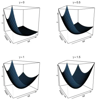
This section seeks to understand the effect of the divergence measure on the weights allocation. Indeed, the choice of the divergence measure can produce different optimal weights. Figure 1 displays the divergence surface between the normal distribution with mean 0 and standard deviation 1, and normal distributions of varying mean and standard deviation. The power divergence family was used, with different sets of exponent values as shown in the figure. It is clear that the divergence has different shapes, depending upon the power parameter. This is a strong indication that portfolio estimators based on different divergence measures will yield different weight parameter estimates.

The supremum of the dual form of the divergence measure is used to estimate the divergence measure itself. Recall that the supremum of the dual form of the power divergence is obtained when its derivatives are equal to zero, where

dγ(Pw, Pr, Pθ) =

1 n(γ−1)

n X i=1 " fθ fr

γ−1

−1 # −1 γ Z b a fr fθ fr γ −1 du,

δθdγ(Pw, Pr, P_θ) =

1 n

n

X

i=1

∇fθ(xi)

fr(xi)

fθ(xi)

fr(xi)

γ−1

−

Z b

a

∇fθ

fθ

fr

γ−1

mean

sd

z

γ =0

mean

sd

z

γ =0.5

mean

sd

z

γ =1

mean

sd

z

γ =1.5

As noted by Toma and Broniatowski [2011], the summation corresponds to the weighted likelihood score function. The weight function is

fθ(xi)

fr(xi)

γ−1

.

The effect of the choice of the power divergence parameter, γ, upon the optimized weights, can be understood by studying this weight function. Note that forγ = 1, there are no weights, and so the estimator reduces to the maximum likelihood estimator.

Two cases must be distinguished. The first case is when the reference distribution can be described by the data set. The second case is when the data set does not converge in distribution to the reference model.

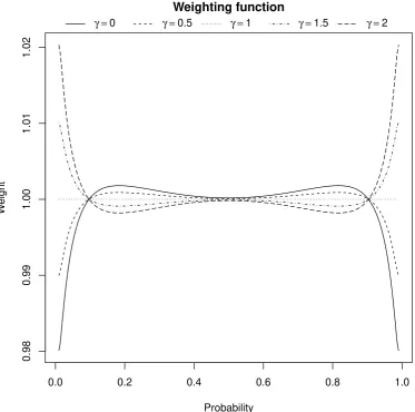
When the portfolio data set converges in distribution to the reference portfolio distribution, the auxiliary distribution in the dual form converges to the reference distribution as well; i.e.,

fθ→fr. The weighting function, [fθ(x)/fr(x)]γ−1, converges to unity, and thus all points are

equally weighted. Figure 2 illustrates this effect; the weight function is close to one for most of the distribution range, irrespective of the gamma factor.

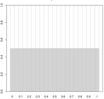
Regarding portfolio allocation, when the portfolio data set can converge in distribution to the reference distribution, the choice of the divergence measure does therefore not change the weights allocation. To illustrate this, two time series were simulated: both from the normal distribution with a mean of 0; one having a standard deviation of 1 and the other having a standard deviation of 10. The reference distribution was taken to be the normal distribution with mean 0 and standard deviation 5. The optimized portfolio should therefore be the equally weighted portfolio. Figure 3 displays the weight plot for a range of power exponents between 0 and 1. The weights remain constant over the range of power exponents.

However, when the data is significantly different from the reference distribution, the likelihood score function is weighted by the likelihood ratio. At the supremum of the dual divergence measure, the auxiliary distribution, fθ, converges in distribution to the portfolio distribution,

fr, as seen in Section 4. The value of the weight function depends on the power exponent γ, if

it is less or greater than 1, and on the likelihood ratio, fθ(xi)

fr(xi), if the likely value of the auxiliary

distribution is less or greater than the one of the reference distribution at xi. Consider the

points with indexiwherefθ(xi)> fr(xi); that is when the reference distribution has thinner

tails than the empirical portfolio. Whenγ >1 (γ <1), the score function is then upweighted (downweighted) at these points. The effect is inverted for values at indexiwherefθ(xi)< fr(xi).

To illustrate this, three cases are considered. The first case is when the reference distribution scale is larger than the data set scale. The second case is when the scale parameter of the reference distribution is smaller than that of the data set. The third case is when the reference distribution has a larger mean than does the data set.

0.0 0.2 0.4 0.6 0.8 1.0

0.98

0.99

1.00

1.01

1.02

Weighting function

Probability

W

eight

γ =0 γ =0.5 γ =1 γ =1.5 γ =2

0 0.1 0.2 0.3 0.4 0.5 0.6 0.7 0.8 0.9 1

0.0

0.2

0.4

0.6

0.8

1.0

Weights Plot

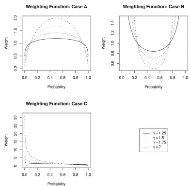
the data set, the divergence portfolio privileges the allocation that produces the best fit in the tails. This effect is increased when reducingγ toward 0. In the case when the target distribution has a smaller scale than the reference distribution, reducingγ towards zero has the effect of increasing the weighting around the center of the distribution.

Whenγ >1, Fig. 5, the effect is inverted as is expected from the form of the weight function, which is to the power γ−1. When the reference distribution has a larger scale than the data set does, the center of the distribution gains higher weighting asγ increases. When the reference distribution has a smaller scale than the data set does, the tail of the distribution has higher weight as γ increases.

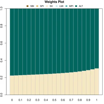
Now to examine the effect of the power parameterγ in the context of portfolio optimization with a real data set; the Swiss Pension Fund Benchmarks1 _{of Pictet is used. The family of}

Pictet LPP indices was created in 1985 with the introduction of new regulations in Switzerland governing the investment of pension fund assets. Since then it has established itself as the authoritative pension fund index for Switzerland. In 2000, a family of three indices, called LPP25, LPP40, and LPP60, where the increasing numbers denote increasingly risky profiles, were introduced to provide a suitable benchmark for Swiss pension funds. It is composed of 6 instruments. In this example, the objective is to find the asset allocation of these 6 assets such that the resulting portfolio is as close as possible to the normal distribution with the mean and standard deviation of the benchmark LPP60. Figure 6 displays the optimal weights obtained for different values of the power divergence.

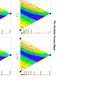
Given that the allocation might change, depending on the choice of the divergence measure, it is of interest to see if the shape of the divergence measure between the empirical portfolio and the reference portfolios might change as well. In this regard, Fig. 7 displays the ternary plot of the divergence measure for the portfolio, with components SBI, SPI and SII, with respect to the reference portfolio. SBI is the Swiss bond index, SPI is the Swiss performance index and SII is the Swiss real estate index. The logarithm returns of these indices with daily records from 2000–01–03 to 2007–05–042 _{were considered. The reference distribution used is the Student}

t-distribution with its parameter-values fitted to the equally weighted portfolio with the SBI, SPI and SII. The four plots have been generated with different power divergence parameters as indicated in the figure. The shape of the divergence measure does not significantly change, although the divergence values themselves are quite different. This is important because it shows that the overall shape of the divergence measure is insensitive to the choice of divergence estimator. This provides an indication of the stability of the approach.

1_{The data set (LPP2005) is available in theRpackage}fEcofin

0.0 0.2 0.4 0.6 0.8 1.0

0.5

1.0

1.5

2.0

Weighting Function: Case A

Probability

W

eight

0.0 0.2 0.4 0.6 0.8 1.0

0.0

0.5

1.0

1.5

2.0

Weighting Function: Case B

Probability

W

eight

0.0 0.2 0.4 0.6 0.8 1.0

0.0

0.5

1.0

1.5

2.0

Weighting Function: Case C

Probability

W

eight

γ =0

γ =0.25

γ =0.5

γ =0.75

0.0 0.2 0.4 0.6 0.8 1.0

0.0

0.5

1.0

1.5

2.0

Weighting Function: Case A

Probability

W

eight

0.0 0.2 0.4 0.6 0.8 1.0

0.6

0.8

1.0

1.2

1.4

Weighting Function: Case B

Probability

W

eight

0.0 0.2 0.4 0.6 0.8 1.0

0

5

10

15

20

25

30

Weighting Function: Case C

Probability

W

eight

γ =1.25

γ =1.5

γ =1.75

γ =2

0 0.1 0.2 0.3 0.4 0.5 0.6 0.7 0.8 0.9 1

0.0

0.2

0.4

0.6

0.8

1.0

Weights Plot

SBI SPI SII LMI MPI ALT

0.0204 0.0282 0.0282 0.0428 0.0428 0.0615 0.0615 0.0845 0.0845 0.117 0.117 0.161 0.161 0.21 0.21 0.284 0.284 0.455 1.02 Rmetrics ● ● ● ● ● ● ● ● ● ● ● ● ●

0.12 0.16 0.21 0.28 0.45

1 1.6 ● ● ● SBI SPI SII γ= 0 0.0223 0.0303 0.0303 0.0467 0.0467 0.0671 0.0671 0.0918 0.0918 0.124 0.124 0.163 0.163 0.215 0.215 0.287 0.287 0.4 0.689 ● ● ● SBI SII γ= 1 3 0.0248 0.0341 0.0341 0.0494 0.0494 0.0719 0.0719 0.0981 0.0981 0.134 0.134 0.18 0.18 0.235 0.311 0.311 0.412 0.412 0.563 Rmetrics ● ● ● ● ● ● ● ● ● ● ● ● ●

0.13 0.18 0.24 0.31 0.41 0.56 0.76

● ● ● SBI SPI SII γ= 2 3 0.0274 0.038 0.038 0.0569 0.0569 0.077 0.077 0.107 0.107 0.147 0.147 0.204 0.204 0.273 0.273 0.351 0.464

7 Statistical test

Recall that theφ-portfolio seeks the allocation that produces a portfolio that is as close as possible to the reference distribution. The closeness is expressed by the divergence measure. The value of the objective function in the φ-portfolio therefore carries valuable information. It says how close one can get to the reference model. This is not the case for traditional portfolio allocation.

Cressie and Read [1984] established the asymptotic null distribution of the goodness-of-fit statistics within the power divergence family. They show that the t-test is linked to the χ2

distribution. Broniatowski and Keziou [2009] proved that the asymptotic null distribution of the power divergence family remains aχ2 _{distribution when the divergence measure is expressed in}

its dual form. An important result in [Broniatowski and Keziou, 2009, Theorem 3.2.b] is that at the supremum of the dual divergence, which occurs when the auxiliary distribution tends to the distribution of the sample data, the statistic

2n φ′′₍₁₎dˆφ

convergences in distribution to the χ2 _{distribution where d}ˆ_{φ is the supremum of the dual}

divergence. In the case of the power divergence family, we haveφ′′

(1) = 1and the statistics reduces to2ndˆγ.

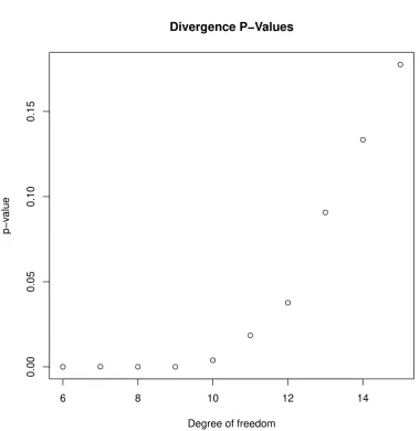
The asymptotic distribution ofφ-divergence statistical tests remains an open research topic. In this context, Jager and Wellner [2007] introduced confidence bands for the power divergence family. The interested reader is referred to their paper and theirRpackage_phitest. Lately, Toma

and Leoni-Aubin [2010] and Toma and Broniatowski [2011] have introduced a more accurate approximation of thep-values of the dual divergence, based on the saddle point approximation of the distribution of the supremum dual divergence as introduced by Robinson et al. [2003] for

M-estimators.

Figure 8 displays the histogram of the statistical tests of the divergence for 1000 time series with the same distribution as the reference distribution that being the normal distribution with mean 0 and standard deviation 1. It is clear from the plot that the statistical test converges in distribution to theχ2 _{distribution.}

Divergence Statistical Test

Density

0 5 10 15

0.00

0.05

0.10

0.15

● ● ● ● ●

●

●

●

●

●

6 8 10 12 14

0.00

0.05

0.10

0.15

Degree of freedom

p−v

alue

Divergence P−Values

8 Expected utility theory

In the expected utility framework, the decision maker constructs a utility function that represents how much the investment would be of interest for him relative to his wealth. The utility function is usually modeled by a concave function that reflects that a smaller gain would be of greater interest to an investor with a smaller wealth. A gain of $1 is of greater interest to an investor who has $10, than to an investor who has $1000. The investor is assumed to be risk-averse and would therefore seek a portfolio allocation that is optimal in a global sense. the investor preference≻is modeled by the stochastic dominance. For two random outcomes, X andY, that belong to a subset of the measurable probability space(Ω,F,P), the preference≻u is defined as

X≻uY ⇐⇒E[u(X)]>E[u(Y)].

The functional form of the expected utility ν(.) = E[u(.)] is known as the expected utility function. When the utility function expresses the risk that the investors are willing to take, then the expected utility functions give a way to measure investor’s preferences.

This section draws the connection between theφ-portfolios and the expected utility theory. Recall that theφ-portfolio is defined as the allocation, w∗_{, for which divergence between the}

portfolio distribution and a reference distribution is smallest:

w∗ _{= arg min} w

Z

φ

fw(x)

fr(x)

fr(x)dx, (9)

where φ is the divergence measure,fw is the empirical distribution of the portfolio given by

the set of weights, w_{, and fr is the reference distribution. When the uniform distribution is}

taken as the reference distribution, the optimal allocation minimizes the expected value of the composition of the divergence φ function and the distribution of the empirical portfolio distribution,φ◦fw. In this case, the optimal weights, w

∗

, are

w∗_{= arg max} w

Z

u(x)dx=E[u(x)] =ν(x), (10)

where u = −φ◦fw. By construction, the function ν is both increasing and concave, and

corresponds to the utility function defined above. The φ-portfolio is thus equivalent to the maximum expected utility portfolio when the reference distribution is the uniform distribution.

It is interesting to note that the Legendre-Fréchet transformation, used here to express to the divergence measure in its dual form, has also been used within the scope of the utility theory [Föllmer and Schied, 2002], where it has been shown that for special choice of the loss function, it reduces to the relative entropy.

The traditional risk-reward portfolio optimization approach can be linked to the utility theory when the risk measures are described as convex functions as shown by De Giorgi [2005]. The

9 Conclusion

This paper has introduced a portfolio allocation scheme based on theφ-divergence measure. The approach uses the dual representation of the divergence measure to avoid using a non-parametric estimation of the empirical distribution. The advantages of the approach are multifold.

As was seen, the scheme seeks the allocation that produces a portfolio that is the closest to a reference model while remaining as compatible as possible to the empirical data, which can be interpreted as a type of Bayesian estimator. This is in contrast to the traditional risk-reward paradigm where an attempt is made to optimize one quantity given constraints. It is believed to be a more viable approach because it reduces the risk estimation error induced by the risk-reward model. In the approach devised in this article, the weights selected are those that are in greatest accord with the empirical data. This could lead to a situation where the selected weights might have a slightly increased deviation, but a much better mean vector. This is also important in the context of robust estimators. As in the case of the power divergence measure, the power exponent can make the estimator more robust to outliers. Given the choice of the divergence measure, the φ-portfolios can be viewed as robust estimators.

Moreover, the value of the optimized φ-portfolio function provides information on how close the investor is to his reference model. It can be used as a statistical test; providing a warning that the reference model might have been too ambitious for the empirical data.

Another important aspect is that the divergence measure is convex and fast optimization routines can be used in practice. This paper has presented the primal-dual interior optimization for estimating the supremum of the dual representation of the divergence measure and to solve the minimumφ-portfolio problem.

The relationship between this new framework and the utility theory has been highlighted. It has been shown that the utility function becomes a particular case of theφ-portfolio when the uniform distribution is chosen as the reference distribution.

Divergence measure is an active research topic. Many problems remain open. There is no clear comparison of the properties for the different functions that have been introduced over the last few decades. Also, a complete asymptotic theory ofφ-divergences has yet to be found. All these open problems constitute a favorable outlook for the practical use ofφ-portfolios. An exhaustive comparison of φ-portfolios to common portfolio optimization schemes would be a valuable contribution to the field.

Acknowledgments

This work is part of the PhD thesis of Yohan Chalabi. He acknowledges financial support from Finance Online GmbH and from the Swiss Federal Institute of Technology Zurich.

References

S. Ali and S. Silvey. A general class of coefficients of divergence of one distribution from another.

J. R. Stat. Soc., Ser. B, 28:131–142, 1966.

F. Black and R. Litterman. Global portfolio optimization. Financial Analysts Journal, pages 28–43, 1992.

M. Broniatowski and A. Keziou. Minimization ofφ-divergences on sets of signed measures. Stud. Sci. Math. Hung., 43(4):403–442, 2006.

M. Broniatowski and A. Keziou. Parametric estimation and tests through divergences and the duality technique. Journal of Multivariate Analysis, 100(1):16–36, 2009.

N. Cressie and T. R. Read. Multinomial goodness-of-fit tests. J. R. Stat. Soc., Ser. B, 46: 440–464, 1984.

I. Csiszár. Eine informationstheoretische Ungleichung und ihre Anwendung auf den Beweis der Ergodizität von Markoffschen Ketten. Publ. Math. Inst. Hung. Acad. Sci., Ser. A, 8:85–108, 1963.

E. De Giorgi. Reward-risk portfolio selection and stochastic dominance. Journal of Banking & Finance, 29(4):895–926, 2005.

P. Fishburn. Mean-risk analysis with risk associated with below-target returns. American Economic Review, 67(2):116–126, 1977.

H. Föllmer and A. Schied. Convex measures of risk and trading constraints. Finance and Stochastics, 6:429–447, 2002.

F. Foster and C. Whiteman. An application of Bayesian option pricing to the Soybean market.

American journal of agricultural economics, 81(3):722–727, 1999.

M. R. Haley and C. H. Whiteman. Generalized safety first and a new twist on portfolio performance. Econometric Reviews, 27(4–6):457–483, 2008.

P. Jorion. Value at risk: the new benchmark for controlling market risk, volume 2. McGraw-Hill New York, 1997.

A. Keziou. Dual representation ofφ-divergences and applications.Comptes Rendus Mathematique, 336(10):857–862, 2003.

Y. Kitamura and M. Stutzer. An information-theoretic alternative to generalized method of moments estimation. Econometrica, 65(4):861–874, July 1997.

S. Kullback and R. A. Leibler. On information and sufficiency. The Annals of Mathematical Statistics, 22(1):79–86, 1951.

F. Liese and I. Vajda. On divergences and informations in statistics and information theory.

Information Theory, IEEE Transactions on, 52(10):4394–4412, Oct. 2006.

B. Lindsay. Efficiency versus robustness - the case for minimum Hellinger distance and related methods. Annals of Statistics, 22(2):1081–1114, June 1994.

P. Mahalanobis. On the generalized distance in statistics. InProceedings of the National Institute of Sciences of India, volume 2, pages 49–55. New Delhi, 1936.

H. Markowitz. Portfolio selection. The Journal of Finance, 7(1):77–91, 1952. H. Markowitz. Portfolio Selection. John Wiley & Sons, New York, 1959.

A. Meucci. Fully flexible views: theory and practice. Risk, 21(10):97–102, 2008.

D. Morales, L. Pardo, and I. Vajda. Some new statistics for testing hypotheses in parametric models. Journal of Multivariate Analysis, 62(1):137–168, July 1997.

D. Morales, L. Pardo, M. Pardo, and I. Vajda. Limit laws for disparities of spacings. Journal of Nonparametric Statistics, 15(3):325–342, June 2003.

T. Morimoto. Markov processes and the H-theorem. J. Phys. Soc. Jap., 18:328–331, 1963. L. Pardo. Statistical Inference Based on Divergence Measures. Taylor & Francis Group, LLC,

2006.

T. R. Read and N. A. Cressie. Goodness-of-fit statistics for discrete multivariate data. New York etc.: Springer-Verlag, 1988.

J. Robertson, E. Tallman, and C. Whiteman. Forecasting using relative entropy. Journal of Money Credit and Banking, 37(3):383–401, June 2005.

R. Rockafellar and S. Uryasev. Optimization of conditional value-at-risk. Journal of risk, 2: 21–42, 2000.

A. D. Roy. Safety first and the holding of assets. Econometrica, 20(3):431–449, 1952.

C. Shannon. A mathematical theory of communication. Bell System Technical Journal, 27(3): 379–423, 1948.

F. Sortino and R. Van Der Meer. Downside risk. The Journal of Portfolio Management, 17(4): 27–31, 1991.

M. Stutzer. A simple nonparametric approach to derivative security valuation. Journal of Finance, 51(5):1633–1652, Dec. 1996.

M. Stutzer. A portfolio performance index. Financial Analysts Journal, 56(3):52, 2000.

A. Toma and M. Broniatowski. Dual divergence estimators and tests: Robustness results.

Journal of Multivariate Analysis, 102(1):20–36, 2011.

A. Toma and S. Leoni-Aubin. Robust tests based on dual divergence estimators and saddlepoint approximations. Journal of Multivariate Analysis, 101(5):1143–1155, 2010.

I. Vajda. Theory of statistical inference and information. Dordrecht etc.: Kluwer Academic Publishers, 1989.