https://doi.org/10.1007/s10955-019-02340-1
Rare Event Simulation for Stochastic Dynamics in Continuous
Time
Letizia Angeli1 ·Stefan Grosskinsky1 ·Adam M. Johansen1 · Andrea Pizzoferrato2
Received: 2 October 2018 / Accepted: 11 June 2019 © The Author(s) 2019
Abstract
Large deviations for additive path functionals of stochastic dynamics and related numerical approaches have attracted significant recent research interest. We focus on the question of convergence properties for cloning algorithms in continuous time, and establish connections to the literature of particle filters and sequential Monte Carlo methods. This enables us to derive rigorous convergence bounds for cloning algorithms which we report in this paper, with details of proofs given in a further publication. The tilted generator characterizing the large deviation rate function can be associated to non-linear processes which give rise to several representations of the dynamics and additional freedom for associated numerical approximations. We discuss these choices in detail, and combine insights from the filtering literature and cloning algorithms to compare different approaches and improve efficiency.
Keywords Dynamic large deviations·Interacting particle systems·Cloning algorithm· Sequential Monte Carlo
1 Introduction
Large deviation simulation techniques based on classical ideas of evolutionary algorithms [1,2] have been proposed under the name of ‘cloning algorithms’ in [3] for discrete and in [4] for continuous time processes, in order to study rare events of dynamic observables of interacting lattice gases. This approach has subsequently been applied in a wide variety of contexts (see e.g. [5–8] and references therein), and more recently, the convergence properties of the algorithm have become a subject of interest. Analytical approaches so far are based on a branching process interpretation of the algorithm in discrete time [9], with limited and mostly numerical results in continuous time [10]. Systematic errors arise from the correlation
Communicated by Abhishek Dhar.
B
Stefan Grosskinsky1 University of Warwick, Coventry, UK
structure of the cloning ensemble which can be large in practice, and several variants of the approach have been proposed to address those including e.g. a multicanonical feedback control [7], adaptive sampling methods [11] or systematic resampling [12]. A recent survey of these issues and different variants of cloning algorithms in discrete and continuous time can be found in [13, Sect. 3].
In this paper we provide a novel perspective on the underlying structure of the cloning algorithm, which is in fact well established in the statistics and applied probability literature on Feynman–Kac models and particle filters [14–16]. The framework we develop here can be used to generalize rigorous convergence results in [17] to the setting of continuous-time cloning algorithms as introduced in [4]. Full mathematical details of this work are published in [18], and here we focus on describing the underlying approach and report the main convergence results. A second motivation is to use different McKean interpretations of Feynman–Kac semigroups (see Sect.2.2) to highlight several degrees of freedom in the design of cloning-type algorithms that can be used to improve performance. We illustrate this with the example of current large deviations for the inclusion process (originally introduced in [19]), aspects of which have previously been studied [20]. Current fluctuations in stochastic lattice gases have attracted significant recent research interest (see e.g. [21–23] and references therein), and are one of the main application areas of cloning algorithms which are particularly challenging. In contrast to previous work in the context of cloning algorithms [9,10], our mathematical approach does not require a time discretization and works in a very general setting of a jump Markov process on a compact state space. This covers in particular any finite state Markov chain or stochastic lattice gas on a finite lattice.
The paper is organized as follows. In Sect.2we introduce notation, the Feynman–Kac semigroup and several representations of the associated non-linear process. In Sect.3we describe different particle approximations including the cloning algorithm, and summarize results published in [18] on convergence properties of estimators based on the latter. In Sect.4 we describe a modification of the cloning algorithm for a particular class of stochastic lattice gases and apply it to the inclusion process as an example.
2 Mathematical Setting
2.1 Large Deviations and the Tilted Generator
We consider a continuous-time Markov jump processX(t):t≥0on a compact state space
E. To fix ideas we can think of a finite state Markov chain, such as a stochastic lattice gas on a finite latticewith a fixed number of particlesM. HereEis of the formSwith a finite setSof local states (e.g.S = {0,1}or{0, . . . ,M}), but continuous settings with compact E⊂Rd for anyd ≥1 are also included. One can in principle also generalize to separable and locally compact state spaces, including countable Markov chains and lattice gases on finite lattices with open boundaries. But this would require more effort and complicate not only the proof but also the presentation of the main results for technical reasons which we want to avoid here (see [18] for a more detailed discussion).
Jump rates are given by the kernelW(x,d y), such that for allx ∈ E and measurable subsetsA⊂E
PX(t+t)∈AX(t)=x=t
A
whereo(t)/t → 0. We use the standard notationPandEfor the distribution and the corresponding expectation on the usual path space for jump processes
=ω: [0,∞)→Eright continuous with left limits .
If we want to stress a particular initial conditionx ∈ Eof the process we writePxandEx. The process can be characterized by the infinitesimal generator
Lf(x)=
E
W(x,d y)[f(y)− f(x)], ∀f ∈Cb(E),x∈E, (2.2)
acting on all continuous bounded functions f ∈Cb(E)on the state space. The adjointL†of this operator acts on probability distributionsμonE, and determines their time evolution via
d
dtμt(d y)=
x∈E
μt(d x)W(x,d y)−
x∈E
μt(d y)W(y,d x), (2.3)
whereP[Xt ∈ A] =
Aμt(d y)for any regularA⊂ Echaracterizes the distribution of the process at timet≥0. In case of countableE, (2.3) is simply the usual master equation of the process forμt(y)=P[Xt=y], but we focus our presentation on the equivalent description via the generator (2.2), which leads to a more compact notation and applies in the general setting. As a technical assumption we require that the total exit rate of the process is uniformly bounded
w(x):=
E
W(x,d y)≤ ¯w <∞ for allx ∈E. (2.4)
We are interested in the large deviations of additive path space observablesAT :→R of the general form
AT(ω):=
t≤T
ω(t−) =ω(t)
gω(t−), ω(t)+
T
0
hω(t)dt, (2.5)
whereg ∈Cb(E2)andh ∈Cb(E). Note thatAT is well defined since the bound onw(x) implies that the sum in the first term almost surely contains only finitely many terms for any
T >0. The above functional, which recently appeared in this form in [24], assigns a weight via the functiongto jumps of the process, as well as to the local time via the functionh. Dynamics conditioned on such a functional have been studied in many contexts [5], including driven diffusions on periodic continuous spacesE[25].
As mentioned before, the simplest examples covered by our setting are Markov chains with finite state space E. This includes stochastic particle systems on a finite lattice with periodic or closed boundary conditions such as zero-range or inclusion processes [20,23,26], and also processes with open boundaries and bounded local state space such as the exclusion process [3]. Choosinggappropriately andh≡0 the functionalATcan, for example, measure the empirical particle current across a bond of the lattice or within the whole system up to timeT.
We assume thatATadmits a large deviation rate function, which is a lower semi-continuous functionI:R→ [0,∞]such that
lim T→∞−
1
convexity ofI can be established in a very general setting for countable state space (see e.g. [29] and references therein). IfI is convex, it is characterized by the scaled cumulant generating function (SCGF)
λk := lim T→∞
1
T logE
ek AT (2.7)
via the Legendre transform
I(a)=sup k∈R
ka−λk
. (2.8)
It is well known (see e.g. [24,26]) thatλkcan be characterized as the principal eigenvalue of a tilted version of the generator (2.2)
Lkf(x):=
E
W(x,d y)ekg(x,y)f(y)− f(x)+kh(x)f(x)
=
E
Wk(x,d y)
f(y)− f(x)
=:Lk f(x)
+Vk(x)f(x) (2.9)
with modified rates for the jump partLˆk
Wk(x,d y):=W(x,d y)ekg(x,y), (2.10) and potential for the diagonal part
Vk(x):=
E
W(x,d y)ekg(x,y)−1+kh(x). (2.11)
By (2.4) and the boundedness ofgandh, for eachk∈Rthere exist constants such that we have uniform bounds
E
Wk(x,d y)≤ ¯wk and Vk(x)≤ ¯vk for allx ∈E. (2.12)
Note also thatL0 =L, but for anyk =0 the diagonal part of the operator does not vanish
and
Lk1(x)=Vk(x) for allx ∈E. (2.13)
Still, it generates a Feynman–Kac semigroup (see e.g. [17,24] for details), defined as
Ptkf(x)=etLkf(x):=Ex
f ek At, (2.14)
which is the unique solution to the backward equation
d
dtP
k
t f = Ptk(Lkf) with P0kf = f. (2.15)
Due to the diagonal part ofLkthis does not conserve probability, i.e. for the constant function
f ≡1 we get
Ptk1(x)=Ex
ek At =1 for allk =0, t>0. (2.16) The associated logarithmic growth rate
λk(t):= 1
t logP
k
t1(x) (2.17)
provides a finite-time approximation of the SCGFλk, which depends on the initial condition
property of the process, discussed in detail in [18] and references therein. Under exponential mixing assumptions, which are mild in our contexts of interest, it can be shown that for some constantC>0
λk(t)−λk≤C/t ast→ ∞. (2.18)
This is for example the case ifEis finite and the process necessarily has a spectral gap, as is the case for all finite state lattice gases mentioned earlier. Furthermore, exponential mixing implies that the modified finite-time approximation
λk(at,t):= 1
(1−a)t log Ptk1(x)
Patk1(x) witha∈(0,1), (2.19)
with a ’burn-in’ time period of lengthat, significantly improves the convergence in (2.18) to
λk(at,t)−λk≤Cρat/t ast→ ∞ (2.20)
for someρ∈(0,1). This is of course routinely used in Monte–Carlo sampling where systems are allowed to relax towards stationarity before measuring. These intrinsic properties of the process and the related finite-time errors in the estimation ofλk are not the main subject of this paper. In the following we simply assume asymptotic stability and (2.18), and focus on the efficient numerical estimation ofλk(t)for any givent ≥0.λk(at,t)can be treated completely analogously, which is discussed in more detail in [18].
2.2 McKean Interpretation of the Feynman–Kac Semigroup
As usual, for a given initial distributionν0konEthe semigroup (2.14) determines a measure
νk
t at timest≥0 onE, which can be characterized weakly through integrals of bounded test functions f ∈Cb(E)as
νk t(f):=
E
f(x)νtk(d x)=
E
Ptkf(x)ν0k(d x). (2.21)
Here and in the following we use the common short notationνtk(f)for the integral of the function f under the measureνkt to simplify notation. Note that we can write (2.17) as
λk(t)= 1
t logν
k
t(1), (2.22)
with a more general initial conditionν0k. But sincePtkdoes not conserve probability,νtkis not a normalized probability measure and it is consequently impossible to sample from it.
With (2.16)νk
t(1) >0 for allt≥0, and we can define normalized versions of the measures via
μk
t(f):=νkt(f)/νkt(1). (2.23) Using (2.9), (2.13) and (2.15) on can derive the evolution equation
d
dtμ
k t(f)=
d dt
νk t(f)
νk t(1)
= 1
νk t(1)
νk
t(Lkf)− ν k t(f)
νk t(1)2
νk t(Lk1) =μk
t(Lkf)−μtk(f) μkt(Lk1) =μk
with initial conditionμk0=νk0. It can be shown by similar direct computation ofdtd logνtk(1), using (2.13) and (2.22) that
λk(t)= 1
t
t
0
μk
s(Vk)ds. (2.25)
So the finite-time approximation ofλk is given by an ergodic average with respect to the distributionμkt, depending on the initial distributionμk0, with an obvious modification for (2.19). The asymptotic stability of the original process implies thatμk
t →μk∞converges to a unique stationary distributionμk∞onE, so that the SCGF (2.7) can be written as the stationary expectation of the potential
λk=μk∞(Vk).
Due to the non-linear nature of (2.24),μk∞is characterized by stationarity as the solution of the non-linear equation
μk
∞(Lkf)=μk∞(f) μk∞(Vk)−μk∞(Vkf) for all f ∈Cb(E).
Usuallyμk∞cannot be evaluated explicitly, but from (2.24) it is possible to define a generic processesXk(t) : t ≥ 0
with time-marginals μkt, and then use Monte Carlo sampling techniques. The first term of (2.24) already corresponds to a jump process with generatorLk, and we have to rewrite the second non-linear part to be of the form of a generator. There is some freedom at this stage, and we report three common choices from the applied probability literature on particle approximations [17,30], one of which corresponds to the approach in [3,4], and to the best of the authors’ knowledge the other two have not been considered in the computational physics literature so far.
For every probability distributionμonEwe can write
μ(Vkf)−μ(f) μ(Vk) = μ
L−k,μ,cf +L+k,μ,cf, (2.26)
where
L−k,μ,cf(x):=Vk(x)−c
−
E
f(y)− f(x)μ(d y) (2.27)
and
L+k,μ,cf(x):=
E
Vk(y)−c
+
f(y)− f(x)μ(d y), (2.28)
using the standard notationa+=max{0,a}anda−=max{0,−a}for positive and negative part ofa ∈ R. We have the freedom to introduce an arbitrary constantc ∈ R, possibly depending also on the measureμ(but not the statex ∈E), since the left-hand side of (2.26) is invariant under renormalization of the potentialVk(x)→Vk(x)−c. The generatorsL−k,μ,c andL+k,μ,cdescribe jump processes onEwith rates depending on the probability measure
μ.Vk(x)can be interpreted as a fitness potential for the process, and play exactly that role in the particle approximation of this process based on population dynamics, which is presented in Sect.3. Generic choices are:
• c=0 is the default and simplest choice, but is usually not optimal as discussed in Sect.4. • c = μkt(Vk)corresponding to the average potential: If the system in statex is less fit
thancit jumps to stateychosen from the distributionμk
t(d y)according to (2.27), and independently, the system jumps to states fitter thanc irrespective of its current state according to (2.28).
Another representation of the non-linear part in (2.24) is (see e.g. [31, Sect. 5.3.1])
LVk,μf(x):=
E
Vk(y)−Vk(x)
+
f(y)− f(x)μ(d y), (2.29)
which is particularly interesting for implementing efficient selection dynamics as discussed in Sect.4. Here every jump from this part of the generator strictly increases the fitness of the process, which is a stronger version of the previous idea where the process on average increased its fitness above levelc. The rate depends on departure statex and target state
y, which is in general computationally more expensive to implement than rates in (2.27) and (2.28), but can still be feasible due to simplifications in many concrete examples as demonstrated in Sect.4. A further improvement of that idea is given by
LVk,μf(x):=
Vk(x)−μ(Vk)
−
E
Vk(y)−μ(Vk)
+
μ(Vk−μ(Vk))+
f(y)− f(x)μ(d y), (2.30)
which resembles a continuous-time version of selection processes which are known under the names of stochastic remainder sampling [32] or residual sampling [33] in discrete time. Here selection events change the process from statesxof less than average fitnessμ(Vk)to statesyfitter than average, but we will see in Sect.4that this variant is harder to implement than (2.29) in our area of interest, and offers only limited extra gain in selection efficiency.
In summary, the evolution equation (2.24) forμkt can be written as
d
dtμ
k
t(f)=μkt(Lkf)+μt(LVk,μt f) (2.31)
where the first choice with (2.27) and (2.28) is included definingLVk,μ=L−k,μ,c+L+k,μ,cin that case. This defines a Markov processXk(t):t≥0
on the state spaceEwith generator
Lk,μk
t f(x):=Lkf(x)+L V
k,μkt f(x). (2.32) The process is non-linear since the transition rates in the generatorLk,μk
t depend on the distri-butionμkt of the process at timet, and in particular the process is also time-inhomogeneous. While the generator is still a linear operator acting on test functions f, the adjointL†
k,μkt is a
non-linear operator acting on measuresμkt, generating their time evolution via
d
dtμ
k
t(d y)=L
†
k,μk tμ
k
t, (2.33)
which is equivalent to (2.31). This microscopic mass transport description consistent with the macroscopic description provided by the Feynman–Kac semigroupPk
t is also called a McKean representation [16,31]. It is well know that particle approximations of different McKean representations can have very different properties. The first part is similar to the original dynamics with modified ratesWk(2.10), and the second non-linear part depending on the distributionμkt arises from normalizing the measuresνtk. Note thatμkt and therefore the finite-time approximationλk(t)in (2.25) are uniquely determined by (2.24), and thus independent of the different McKean representations, as are of course the limiting quantities
μk
∞andλk. Also, these interpretations do not make use of concepts from population dynamics
3 Particle Approximations and the Cloning Algorithm
The rates of the non-linear processXk(t) :t ≥ 0
(2.32) depend on the distributionμt, which is not known a-priori in the cases in which we are interested. The natural framework to sample such non-linear processes approximately is a particle approximation, see e.g. [30]. Here an ensembleXk(t) : t ≥ 0ofN processes (also called particles or clones)Xik(t),
i=1, . . . ,Nis run in parallel on the state spaceEN, andμktis approximated by the empirical distributionμN(Xk(t))of the realizations, where for anyx∈EN we define
μN(x)(d y):= 1
N
N
i=1
δxi(d y) as a distribution onE. (3.1)
SinceμN(Xk(t))is fully determined by the state of the ensemble at timet, the particle approximation is a standard (linear) Markov process onEN. This leads to an estimator for the SCGF using (2.25) given by
N k(t):=
1
t
t
0
μN(X
k(s))(Vk)ds= 1
t
t
0
1
N
N
i=1
Vk(Xik(s))ds, (3.2)
which is a random object depending on the realization of the particle approximation. The full dynamics can be set up in various different ways such thatμN(Xk(t))→μkt converges as
N → ∞for anyt≥0. A generic version, directly related to the above McKean representa-tions has been studied in the applied probability literature in great detail [17,30], providing quantitative control on error bounds for convergence. After describing this approach, we present a different approach known in the theoretical physics literature under the name of cloning algorithms [5,13], which provides some computational advantages but lacks general rigorous error control so far [9,10]. We will then set up a framework to identify common aspects of both approaches, which can be used to generalize existing convergence results to obtain rigorous error bounds for cloning algorithms as described in detail in [18], and to compare computational efficiency of both approaches.
3.1 Basic Particle Approximations
The most basic particle approximation is simply to run the McKean dynamics (2.32) in parallel on each of the particles, replacing the dependence onμkt byμN(Xk(t))in the jump rates. Mathematically, denoting byLNk the generator of the fullNparticle processXk(t):t≥0 acting on functionsF:EN →R, this corresponds to
LN
k F(x):= N
i=1
Li
k,μN(x)F(x). (3.3)
HereLik,μN(x)is equivalent to (2.32) acting on particleionly, i.e. on the functionxi →F(x) whilexj,j =iremain fixed. The linear partL
L−,i
k,μN(x),cF(x)=
Vk(xi)−c
−
E
F(xi,y)−F(x)μN(x)(d y)
=Vk(xi)−c
− 1 N N j=1
F(xi,xj)−F(x) (3.4)
with notationxi,y=(x1, . . . ,xi−1,y,xi+1, . . . ,xN). So with a rate depending on the fitness of particlei, it is ‘killed’ and replaced by a copy of particle j uniformly chosen from all particles. Analogously, we have for (2.28)
L+,i
k,μN(x),cF(x)= 1
N
N
j=1
Vk(xj)−c
+
F(xi,xj)−F(x), (3.5)
which leads to the same transitionx →xi,xj, but with a different interpretation. Each particle
jin the system reproduces independently with a rate depending on its fitness (cloning event), and its offspring replaces a uniformly chosen particle, which is equal toi with probability 1/N. The different nature of killing and cloning events becomes clearer when we write out the full generator (3.3) and switch summation indices for the cloning part (3.5) in the second line,
LN kF(x)=
N
i=1
E
Wk(xi,d y)
F(xi,y)−F(x)
+ N
i=1
Vk(xi)−c
+ 1 N N j=1
F(xj,xi)−F(x)
+ N
i=1
Vk(xi)−c
− 1 N N j=1
F(xi,xj)−F(x). (3.6)
Analogously, the McKean representations (2.29) and (2.30) lead to basicN-particle systems with generators
LN k F(x)=
N
i=1
E
Wk(xi,d y)
F(xi,y)−F(x)
+ 1
N
N
i,j=1
Vk(xj)−Vk(xi)
+F(xi,xj)−F(x) (3.7)
and
LN k F(x)=
N
i=1
E
Wk(xi,d y)
F(xi,y)−F(x)
+ 1
N
N
i,j=1
Vk(xi)−μ(Vk)
−Vk(xj)−μ(Vk)
+
μ(Vk−μ(Vk))+
F(xi,xj)−F(x). (3.8)
Following established results in [17,30,31], the (random) quantitykN(t)is an asymptot-ically unbiased estimator ofλk(t)with a systematic error bounded by
sup t≥0 ENN
k(t)
−λk(t)≤
C
N for allN ≥1, (3.9)
along with several rigorous convergence results. These include an estimate on the random error inLpnorm for anyp>1,
sup t≥0E
N|N
k(t)−λk(t)|p
1/p ≤ Cp
√
N for allN ≥1, (3.10)
as well as other formulations including almost sure convergence. Note that these estimates are uniform int≥0, so are not affected by the choice of simulation time. The use of a finite simulation time,t, leads to an additional systematic error to the estimate of the SCGFλk, of order 1/tas in (2.18) orρat/tas in (2.20). The bound (3.10) for p=2 implies for the variance
sup t≥0
ENN
k(t)−EN
N k(t)
2
≤ C22
N for allN ≥1, (3.11)
since we have Var(Y)=infa∈RE(Y−a)2for any real-valued random variableY. There-fore, error bars based on standard deviations are of the usual Monte Carlo order of 1/√N, and the random error dominates the systematic bias (3.9) forN large enough. Further remarks on possible unbiased estimators can be found at the end of the next subsection.
3.2 Essential Properties of Particle Approximations
Following the standard martingale characterization of Feller-type Markov processes (see e.g. [34], Chap. 3), we know that for every bounded, continuousF∈Cb(EN)
MN
F(t):=F
Xk(t)−FXk(0)−
t
0
LN k F
Xk(s)ds (3.12)
is a martingale onRwith (predictable) quadratic variation
MN F(t)=
t
0
N k F
Xk(s)ds, (3.13)
where the associated carré du champ operatorkN is given by
N
k F(x):=LkNF2(x)−2F(x)LkNF(x). (3.14) In analogy to the decomposition of a random variable into its mean and a centred fluctuating part, the martingale (3.12) describes the fluctuations of the processt → FXk(t). The strength of the noise depends on time and is given by the increasing process (3.13), whose time evolution is generated by the carré du champ operator (3.14). In contrast to the generator
LN
k, this is a quadratic (non-linear) operator and it is the main tool for studying the fluctuations of a process.
Elementary computations for approximations (3.6), (3.7) and (3.8) show that for marginal test functionsF(x)= f(xi)depending only on a single particle, we have
LN
So generator and carré du champ both coincide with the corresponding operatorsLk,μN(x) andk,μN(x) for the McKean dynamics (2.32). This means that for large enough N and
μNX k(t)
close toμkt, each marginal processt → Xik(t)has essentially the same distri-bution as the corresponding McKean processt → Xk(t). Note that due to selection events these (auxiliary) dynamics do not coincide with the original process conditioned on a large deviation event, and they are also not unique since there are various choices for McKean representations of Feynman–Kac semigroups, as discussed earlier. Trajectories in a particle approximation always correspond to the trajectories of the particular McKean interpreta-tion they are based on, which is usually (2.26) in the context of cloning algorithms. Due to asymptotic stability the particle approximation converges ast → ∞for fixedN to a unique stationary distributionμ∞N,k, and the single-particle marginals of this distribution converge toμk
∞ as N → ∞. While the marginal processes for a given particle approximation are
identically distributed they are not independent, andμN∞,k exhibits non-trivial correlations between particles resulting from selection events, which we discuss again in Sect.4.
Now consider averaged observables of the form
F(x)= 1 N
N
i=1
f(xi)=μN(x)(f)
as they appear in the eigenvalue estimator (3.2). Since the generatorLNk is a linear operator inF, we have the same identity as above for the generator,
LN
kμN(x)(f)=μN(x)
Lk,μN(x)f
. (3.15)
The carré du champ, on the other hand, is non-linear in F and the dependence between particles is captured by this operator. Since for all approximations (3.6), (3.7) and (3.8) in every selection event only a single particle is affected, another elementary, slightly more cumbersome computation shows (see [18] for details)
N
k μN(x)(f)= 1
Nμ
N(x) k,μN(x)f
. (3.16)
The factor 1/N results from a self-averaging property of the mean-field interaction through selection dynamics, which is expected from results on other mean-field particle systems (see e.g. [35,36] and references therein), and is fully analogous to the central-limit type scaling of the empirical variance for the sum ofNindependent random variables. While this scaling remains the same for more general particle approximations with more than one particle being affected by selection events, the simple identity (3.16) does not hold exactly for anyN ≥1 as we see in the next subsection.
Recall that the estimator (3.2) for the principal eigenvalue (2.7) is given by an ergodic integral of the average observableF(x) =μN(x)(Vk). With (2.12)Vk ∈Cb(E)and rates are bounded, soμN(x)k,μN(x)Vk
is also bounded and the carré du champ (3.16) vanishes as N → ∞. Therefore the martingaleMNF(t) also vanishes1 for allt ≥ 0, leading to a convergence of the measuresμN(X
k(t))→μkt(t)and also of finite time approximations
N
k(t) → λk(t)as reported in the previous subsection. Due to the time-normalization in (3.2) and the assumed ergodicity, corresponding error bounds hold uniformly int ≥ 0. In summary, bounds on the carré du champ are the main ingredient for the proof of conver-gence results as explained in detail in [18] and references therein. All above properties up to and including (3.15) are generic requirements for any particle approximation. These particle
approximations can differ in their correlation structures and this freedom can be used to con-struct numerically more efficient particle approximations as discussed in the next subsection. To optimize sampling, particles should ideally evolve in as uncorrelated a fashion as possible; it is not possible to achieve completely independent evolution due to the non-linearity of the underlying McKean process and resulting selection events and mean-field interactions.
Remarks on Unbiased Estimators.Estimators based on expectations w.r.t. the empirical measuresμN
t = μN(Xk(t))usually have a bias, i.e.E
μN t (f)
=μt(f)for f ∈ Cb(E), which vanishes only asymptotically (3.9). This originates from the non-linear time evolution ofμkt (2.24) and associated McKean processes. It is straightforward to derive estimators based on the unnormalized measuresνkt (2.21) that are unbiased. Based on (2.25) and (3.2), we obtain an estimate of the normalizationνtk(1):
νN
t (1):=exp t
0
μN s (Vk)ds
, (3.17)
and then introduce unnormalized empirical measures on Eat timet based on the particle approximation
νN
t (f):=νtN(1)μtN(f) for all f ∈Cb(E). The expected time evolution of observables f is then given by
d dtE
νN t (f)
=EνN
t (f)μNt (Vk)+νtN(1)LkNμNt (f)
. (3.18)
Now with (3.15) and the decomposition (2.32) ofLk,μN
t into mutation and selection part, we have
LN
kμtN(f)=μtNLkf +LVk,μN t f
,
and with the general construction of McKean representations (2.26)
μN t (LVk,μN
t f)=μ N
t (Vkf)−μtN(f)μtN(Vk). Inserting into (3.18), this simplifies to
d dtE
νN t (f)
=EνN
t (Lkf)+νtN(Vkf)
.
Since with (2.15)Lk=Lk+Vkalso generates the time evolution ofνt(f), a simple Gronwall argument withEν0N(f)=ν0(f)gives
EνN t (f)
=νt(f) for allt≥0 andN ≥1. (3.19)
Note that choosing f ≡1 implies that the normalization (3.17) is an unbiased estimator ofetλk(t), which we will see again in Sect.3.4in the context of cloning algorithms. However, in practice the random error dominates the accuracy of estimates ofλk(t), soN has to be chosen large and the bias of the estimatorkN(t)(3.2) is negligible.
3.3 Cloning Algorithms
algorithm proposed in [4], but other continuous-time versions can be analysed analogously. The idea is simply to sample the cloning process for each particleitogether with the mutation process at the same rate
wk(xi):=
E
Wk(xi,d y)=
E
w(xi,d y)ekg(xi,y).
In each combined event, a random number of clones is generated with a distributionpkN,x
i(n) such that its expectation is
mNk(xi):= N
n=0
npkN,xi(n)=Vk(xi)−c
+/w
k(xi). (3.20)
These clones then replacenparticles chosen uniformly at random (in the sense that all subsets of sizenare equally probable) from the ensemble. In this way, the rate at which a clone of particleireplaces any given particle jis
wk(xi)
mkN(xi)
N =
1
N
Vk(xi)−c
+
,
as required forLkN in (3.6). The only additional assumption on pkN,xi(n)is that the range of possible values fornhas to be bounded byNfor the cloning event to be well defined. Since its mean is bounded by maxx∈E
Vk(x)−c
+
/wk(x) <∞independently ofN, any distribution with the correct mean and finite range will lead to a valid algorithm for sufficiently largeN.
The above cloning process is described by the generator
LN,mc k F(x):=
N
i=1
N
n=0 1
N
n
A⊆{1,..,N} |A|=n
E
Wk(xi,d y)pkN,xi(n)
F(xA,xi;i,y)−F(x). (3.21)
Here we have used the notationxA,w;i,yfor the vectorz∈EN with
zj :=
⎧ ⎪ ⎨ ⎪ ⎩
xj j ∈/ A∪ {i}
w j ∈A\ {i}
y j =i,
for j ∈ {1, . . . ,N}andw,y ∈ E. (3.21) combines cloning ofxi into a uniformly chosen subsetAof sizen, with a subsequent mutation event where the state of particleichanges to
y. If we simply writeLNk,−for the killing part (third line in (3.6)) which remains unchanged, the full generator of this cloning algorithm is given by
LN,clone
k :=L
N,mc
k +L
N,−
k . (3.22)
It can be shown by direct computation that for marginal test functions of the formF(x)= f(xi)this is equivalent to the generator (3.6)
LN
k F(x)=L N,clone
k F(x), (3.23)
in the correlation structure between particles is picked up by the carré du champ operator. Instead of (3.16) one can derive the following estimate for the mutation and cloning part
N,mc k F(x)≤
2
Nμ
N(x)
kf +1(Vk>c)
qkN
mNk
+
k,μN(x),cf
,
see [18], the proof of Theorem 3.3. HereqkN(xi):=
N
n=0n2pkN,xi(n)denotes the second moment of the number of clones for the particlei, and we use the decomposition (2.32) wherekf is the carré du champ corresponding to the mutation dynamicsLk, andk+,μN(x),c the one corresponding to the cloning part (2.28). This estimate holds, of course, only forN large enough that the cloning event is well defined (see Sect.5). Note also that+
k,μN(x),cf(x)is proportional to(Vk(x)−c)+ and with (3.20)(Vk(x)−c)+=0 impliesmkN(x)=0 for the expectation of the distribution
pkN,x, leading to the indicator function1(Vk>c)∈ {0,1}.
This is sufficient to carry out the full proof of the convergence results mentioned in Sect.3 based on results in [17]. This is carried out in [18] in full detail, and here we only report the main result of that work. Recall the bounds (2.12) onVkand the total modified exit ratewk.
Theorem Denote by ¯kN(t)the eigenvalue estimator (3.2) corresponding to the cloning algorithm(3.22). Then there exist constantsα, γ >0andαp, γp >0such that for all N
large enough
sup t≥0 EN¯N
k(t)
−λk(t)≤ α
Nv¯kw¯k
γ+ qkN∞, (3.24)
and for all p>1
sup t≥0
EN| ¯N
k(t)−λk(t)|p
1/p ≤ αp
√
Nv¯kw¯k
γp+ qkN∞
1/2
. (3.25)
Remarks • Choosing the normalization of the potentialc<infx∈EVk(x)the killing rate in (3.6) vanishes and (3.21) describes the full generatorLN,clone
k for the cloning algo-rithm. This is computationally cheaper and simpler to implement, since only the mutation process has to be sampled independently for all particles, and cloning events happen simultaneously. However, as is discussed in Sect.4, this choice in general reduces the accuracy of the estimator.
• A common choice in the physics literature for the distribution pkN,x
i of the clone size event (see e.g. [3,13]) is
pkN,x
i(n)=
⎧ ⎨ ⎩
mNk(xi)− mNk(xi), forn= mNk(xi) +1 mNk(xi) +1−mkN(xi), forn= mNk(xi)
0, otherwise
, (3.26)
so the two adjacent integers to the mean are chosen with appropriate probabilities, which minimizes the variance of the distribution for a given mean. This choice therefore min-imizes the contribution of the second momentqkN to the bound for the errors in (3.24) and (3.25), and is also simple to implement in practice.
3.4 The Cloning Factor
In the physics literature an alternative estimator toN
t (3.2) is often used, based on a concept called the ‘cloning factor’ (see e.g. [3,5,13]). This is essentially a continuous-time jump process(CkN(t) : t ≥ 0)onR+ withCkN(0) = 1, where at each selection event of size
n≥ −1 at a given timetthe value is updated as
CkN(t)=CkN(t−)(1+n/N). (3.27)
Heren = −1 indicates a killing event, andn ≥ 0 a cloning event according to the two parts of the generator (3.22). This idea comes from a branching process interpretation of the cloning ensemble related to the unnormalized measureνk
t, since with (2.17) we have that
νk
t(1)≈eλkt ast → ∞,
soλk corresponds to the volume expansion factor of the clone ensemble due to selection dynamics.
In our setting, the dynamics ofCkN(t)can be defined jointly with the cloning process via an extension of the generator (3.22)
¯
LN,clone
k F(x, ζ )= ¯L N,mc
k F(x, ζ )+ ¯L N,−
k F(x, ζ ) ,
acting on functions that depend on the statex ∈ EN and the cloning factorζ ∈R+. With (3.21) we have for cloning events
¯
LN,mc
k F(x, ζ ):= N i=1 N n=0 1 N n
A⊆{1,...,N}
|A|=n
E
Wk(xi,d y)pkN,xi(n)
FxA,xi;i,y, ζ(1+n/N)−Fx, ζ
and with the third line of (3.6) for killing events
¯
LN,−
k F(x, ζ )= N
i=1
Vk(xi)−c
− 1
N
N
j=1
F(xi,xj, ζ(1−1/N))−F(x, ζ ).
So the joint process(XNk(t),CkN(t)): t ≥ 0is Markov, and observing only the cloning factor with the simple test functionG(x, ζ )=ζ we get
¯
LN,mc
k G(x, ζ )= N
i=1
N
n=0
1
N
n
A⊆{1,...,N} |A|=n
E
Wk(xi,d y)pkN,xi(n)ζ·
n N =ζ N N i=1
Vk(xi)−c
+
. (3.28)
In the last line we have used (3.20), and in a similar fashion we get for killing events
¯
LN,−
k G(x, ζ )= −
ζ N N i=1
Vk(xi)−c
−
Therefore
¯
LN,clone
k G(x, ζ )=
ζ
N
N
i=1
Vk(xi)−c
=ζmN(x)(Vk)−ζc,
and analogously to (3.18), the expected time evolution ofCkN(t)is then given by
d dtE[C
N
k (t)] =E[CkN(t)·μtN(Vk−c)].
This is also the evolution ofνtN(e−tc)=e−tcνtN(1), since
d dtE[ν
N
t (e−tc)] =E[μtN(Vk)e−tcνtN(1)−c e−tcνtN(1)] =E[νN
t (e−tc)·μtN(Vk−c)].
With initial conditionsCkN(0)=1=νtN(1), a Gronwall argument analogous to (3.19) gives
E[etcCkN(t)] =E[νtN(1)] =νt(1) for allt≥0 andN ≥1.
SoetcCkN(t)is an unbiased estimator forνt(1), which leads also to an alternative estimator forλk(t)(2.17) given by
N k(t):=
1
t logC
N
k(t)+c. (3.30)
Note that this is not itself unbiased as a consequence of the nonlinear transformation involving the logarithm.
SinceCkN(t) is defined as a product (3.27), we can use another simple test function
G(x, ζ )=logζ to analyze the convergence behaviour ofNk(t). Analogously to (3.28) and (3.29) we get
¯
LN,clone
k G(x, ζ )= 1 N N i=1
Vk(xi)−c
=mN(x)(Vk)−c+O
1
N
,
where we have also used (3.20) and assumed that the support ofpkN,x
i is bounded indepen-dently ofN (which is the case for common choices in the literature such as (3.26)). This allows us to approximate log(1+n/N) =n/N +O(1/N2)asN → ∞, leading to error
terms of order 1/N. Then, analogously to (3.12) we get with logCkN(0)=0 that
MN
C(t):=logCkN(t)−
t
0
¯
LN,clone
k G(Xk(s),CkN(s))ds
=logCkN(t)−t(kN(t)−c)+t O
1
N
is a martingale. For the carré du champ we obtain from a straightforward computation that
N,clone
k G(x, ζ )= 1
N2
N
i=1
Vk(xi)−c+O
1
N2
,
and since the potentialVk is bounded (2.12), the quadratic variation of the martingale is bounded by
MN C(t)≤
t N
¯
vk+ |c|
Therefore the estimator (3.30) based on the cloning factor
¯
N k(t)=
1
t logC
N
k(t)+c=kN(t)+O
1
N
+1
tM
N C(t)
is asymptotically equal to the basic estimatorNk(t)(3.2), with corrections that vanish as 1/N
in theLp-norm asN → ∞uniformly int ≥0, analogously to the discussion in Sect.3.2. Therefore, the same convergence results as stated in the Theorem apply for¯Nk(t). Similar convergence results can be shown to hold foretcCkN(t)as an estimator ofνt(1)for fixed
t>0, but naturally cannot hold uniformly in time. Since the object of interest is usually the long-time limitλk(2.17), the practical relevance of this is limited, in addition to the general point that random errors dominate the convergence as mentioned in Sect.3.2. In practice, the basic ergodic averagekN(t)(3.2) is more useful than the cloning factor in the application areas we have in mind. In particular, for alternative particle approximations such as (3.7) or (3.8) where cloning and killing events are effectively combined, it is not clear how to define a cloning factor, whereasNk(t)is always easily accessible.
4 Efficiency and Application of Particle Approximations
4.1 Efficiency of Algorithms
Selection events (cloning or killing) in a particle approximation increase the correlations among the particles in the ensemble, and thereby decrease the resolution in the empirical distribution μNt = μN(Xk(t)), and ultimately the quality of the sample average in the estimator (3.2). Therefore it is desirable to minimize the total rateSk(x)of selection events for a particle approximation. For algorithm (3.6) this is given by
Sk1(x)=
N
i=1
Vk(xi)−c, (4.1)
and the same holds for the cloning algorithm (3.22), since the change in cloning rate is compensated exactly by the average number of clones created to obtain the same overall rate. It is easy to see that for a given state x of the clone ensemble, there is an optimal choice ofc to minimize this expression, given by the median of the fitness distributions
Vk(x):=
Vk(xi):i =1, . . . ,N . If the distribution ofXk(t)is unimodal with light enough tails, the median can be well approximated by the meanμNt (Vk). Since both quantities can be computed with similar computational effort (or well approximated at reduced cost using only a subset of the ensemble), choosing
c=c(t)=medianVk(Xk(t))
should be computationally optimal. In particular, the simplest choicec= 0 in the cloning algorithm is in general far from optimal, so is choosingc =infx∈EVk(x)to get rid of the killing part of the dynamics (see first remark in Sect.3.3).
Sk2(x)= 1 N
N
i,j=1
Vk(xi)−Vk(xj)
+
= 1 2N
N
i,j=1
Vk(xi)−Vk(xj)
≤ 1 2
N
i=1
Vk(xi)−c+c−Vk(xi)=Sk1(x), (4.2)
by symmetry of summations and the triangle inequality. The inequality is strict except for degenerate cases, e.g. ifVk(xi)takes only two values, andclies in between the two. In practice, in the scenarios which we have investigated, it turns out that unless the distribution ofXk(t)
is seriously skewed,S2kis strictly smaller thanSk1by a sizeable amount, as is illustrated later in Fig.2for the inclusion process. Algorithm (3.8) provides further improvement with
Sk3(x)= 1 N
N
i,j=1
Vk(xi)−μN(x)(Vk)
− Vk(xj)−μN(x)(Vk)
+
μN(x)(V
k−μN(x)(Vk))+
= 1 2
N
i=1
Vk(xi)−μN(x)(Vk)≤Sk2(x) . (4.3)
Here we have usediN=1Vk(xi)−μN(x)(Vk)
=0 and Jensen’s inequality to compare with
Sk2(x), sincev→ |a−v|is convex for alla∈R. Note that the rate of change of the mean fitnessμtN(Vk)is given by the same expression in all the above particle approximations,
μN
t (LkVk)+μtN(Vk2)−μtN(Vk)2. (4.4) The first term due to mutation dynamicsLkcan have either sign and is identical in all algo-rithms, while the second due to selection is positive and given by the empirical variance ofVk. This follows from direct computations using the averaged test functionF(x)=μN(x)(Vk) in (3.6), (3.7), (3.8) and (3.22), and is consistent with the evolution equation (2.24). So the mean fitness evolves until a mutation selection balance is reached and the rate of change (4.4) vanishes, characterizing the stationary state of the particle approximation process. Note that this basic mechanism is identical in all particle approximations discussed here, so we expect the mean fitness to show a very similar behaviour. While finite size effects can lead to deviations also in the mean, the main difference between the algorithms is found on the level of variances and time correlations, which can be significantly reduced using (3.7) or (3.8) as illustrated in the next subsections. Since our main observable of interestNk(t)is an ergodic time average ofμtN(Vk), this can lead to significant improvements in the accuracy of the estimator (3.2).
(3.6). While the scalingt NlogN of computational complexity with the sizeNof the clone ensemble is the same, the prefactor and computational cost in practice may be higher and this has to be traded off against gains in accuracy on a case by case basis. For the examples studied below we find a computationally efficient implementation of (3.7) providing a clear improve-ment over the standard cloning algorithm, which is the main contribution of this paper in this context. Algorithm (3.8), on the other hand, provides only marginal improvement over (3.7), but cannot be implemented as efficiently in our area of interest.
4.2 Current Large Deviations for Lattice Gases
In the following we consider one-dimensional stochastic lattice gases with periodic boundary conditions on the discrete torusTLwithLsites and a fixed number of particlesM. Within our general framework, they are simply Markov chains on the finite state spaceE of all particle configurations, which have been of recent research interest in the context of current fluctuations. We denote configurations byη=(ηx :x ∈TL)whereηx∈N0is interpreted as the mass (or number of monomers) at sitex, and the process is denoted as(η(t):t ≥0). In order to use standard notation for lattice gases, in this and the following subsection we change notation, and in particular the use ofx,y ∈ TL is different to the use of those symbols in previous sections where they denoted states inE. Monomers jump to nearest neighbour sites with ratesu(ηx, ηy)≥0 fory=x±1 depending on the occupation numbers of departure and target site, multiplied with a spatial biasp=1−q ∈ [0,1]. The generator is of the form
Lf(η)=
x∈TL
p u(ηx, ηx+1)
f(σx,x+1η)− f(η)
+q u(ηx, ηx−1)
f(σx,x−1η)− f(η)
, (4.5)
whereσx,yη results from the configurationηafter moving one particle fromx to y. The number of particlesM =x∈TLηx is a conserved quantity, but otherwise we assume the process to be irreducible for any fixedM, which is ensured for example by positivity of the rates, i.e. for allk,l≥0
u(k,l)=0 ⇔ k =0.
This class includes various models that have been studied in the literature, for example the inclusion process introduced in [19], where
u(k,l)=k(d+l) for allk,l≥0, (4.6) with a positive parameterd > 0. Particles perform independent jumps with ratedand in addition are attracted by each particle on the target site with rate 1, giving rise to the ‘inclu-sion’ interaction. This model has attracted recent attention due the presence of condensation phenomena [40,41] and in the context of large deviations of the particle current [20], and we will use this as an example in Sect.4.3. Other well-studied models covered by our set-up are the exclusion process with state space E ⊂ {0,1}TL andu(ηx, ηy) = ηx(1−ηy), or zero-range processes withE ⊂ NTL0 and ratesu(ηx, ηy) = u(ηx)depending only on the occupation number on the departure site.
In terms of previous notation, the jump rates for a lattice gas of type (4.5) between any two configurationsηandζare given as
W(η, ζ )=
x∈TL
p u(ηx, ηx+1)δζ,σx,x+1η+q u(ηx, ηx−1)δζ,σx,x−1η
In the following we focus on lattice gases wherexu(ηx, ηx+1)=
xu(ηx, ηx−1)for all configurationsη. While this is not true in general for models of type (4.5), it holds for many examples including inclusion, exclusion and zero-range processes mentioned above. With
p+q=1, the total exit rate out of configurationηis then simply given by
w(η)= x∈TL
p u(ηx, ηx+1)+q u(ηx, ηx−1)
=
x∈TL
u(ηx, ηx+1). (4.8)
We are interested in an observable AT measuring the total particle current up to timeT, which is achieved by choosingh(η)≡0 in (2.5) and
g(η, ζ )= ±1 ifζ =σx,x±1η and g(η, ζ )=0 otherwise.
Using (4.8) we see by direct computation that the potential (2.11) takes the simple form
Vk(η)=(Qk−1)w(η) where Qk:= pek+qe−k. (4.9)
Modified mutation ratesWk(η, ζ )are given by (4.7) replacing(p,q)by(pek,qe−k), leading to modified total exit rates
wk(η)=Qk
x∈TL
u(ηx, ηx+1)=Qkw(η). (4.10)
The similarity ofVk andwkfor lattice gases (4.5) that obey (4.8) provides a direct relation between mutation and selection rates, and allows us to set up an efficient rejection based implementation of a particle approximation(η
k(t):t≥0)based on the efficient algorithm (3.7). In the following we omit the subscriptkfor configurations and writeη(t)=(ηi(t),i=
1, . . . ,N)to simplify notation. For given parameters p,q = 1− pand fixedk ∈ Rwe distinguish two cases.
Qk<1. We sample the ensemble ofN clones at a total rate ofW(η):=
N
i=1w(ηi), and pick a cloneiwith probabilityw(ηi)/W(η)for the next event. With probabilityQk∈(0,1) this is a simple mutation within clonei, and then we replaceηi by ζi with probability
Wk(ηi, ζi)/wk(ηi). Otherwise, with probability 1−Qkwe perform a selection event fol-lowing the second line in (3.7): Pick a clone juniformly at random (includingi). If
Vk(ηj) >Vk(ηi) or equivalently w(ηj) < w(ηi)
(with (4.9) and sinceQk <1), replaceηi byηj with probability
w(ηi)−w(ηj)/w(ηi). This procedure ensures that mutation and selection events are sampled with the correct rates as required in (3.7).
Qk>1. We sample the ensemble ofN clones at a total rate ofQkW(η), and pick a clone
i with probability w(ηi)/W(η) and a clone j uniformly at random. If w(ηj) < w(ηi) we replaceηj byηi with probability Qk−1
Qk
w(ηi)−w(ηj)
w(ηi) . Then we mutate clonei as above, combining the mutation and selection event as in the cloning algorithm.
Remarks Note thatQk=1 is equivalent tok=0, which corresponds to the original process withλ0 = 0 and does not require any estimation. ForQk > 1 we perform mutation and selection events simultaneously, in analogy to the cloning procedure explained in Sect.3.3, but can use the efficient algorithm (3.7). ForQk <1 no mutation or selection event occurs with probability(1−Qk)w(η
j)
Fig. 1 Illustration ofQk(left) as given in (4.9) and the drift 2pek/Qk−1 for the modified dynamics (right)
as a function ofkfor different values of the asymmetryp=1−q. The minimum ofQkis 2√pq, attained at k= 12logqp∈ [−∞,∞], which is also where the modified drift vanishes
Note also that if the cloning algorithm (3.22) is implemented with the common choice
c=0 for a lattice gas of the type discussed here, due to (4.9) and (4.10) the average number of clones per event (3.20) is
mkN(ηi)=Vk(ηi)
+
/wk(ηi)=
Qk−1
Qk ∈(
0,1) ifQk>1,
and 0 forQk<1, where only killing occurs. In particular, this is independent of the stateη of the clone ensemble, and the standard distribution of the form (3.26) is a simple Bernoulli random variable.
While with (4.10) the total mutation rate isQkW(η), selection rates (4.1), (4.2) and (4.3) can be written as
Sk1(η)=
N
i=1
(Qk−1)w(ηi)−cc= |=0 Qk−1|W(η)
Sk2(η)= |Qk−1| 1 2N
N
i,j=1
w(ηi)−w(ηj)
Sk3(η)= |Qk−1| 1 2
N
i=1
w(ηi)−μN(η)(w). (4.11)
So for very small values of Qk close to 0 the mutation rate can become very small in comparison to selection, which means that significant computation time is devoted to re-weighting by selection, rather than advancing the dynamics via mutation events. This effect is typically much stronger for the standard cloning algorithm withc = 0, and occurs for example for totally asymmetric lattice gases withp=1 and negativekconditioning on low currents. In Fig.1we include a sketch ofQkfor different values of asymmetry, including also the drift of the modified dynamics, which can be reversed in partially asymmetric systems.
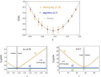
In Fig.2we compare the cloning algorithm to algorithms (3.7) and (3.8) for an inclusion process withd = 1, L = 64, M = 128 and asymmetry p = 0.7. It is known [20] that the SCGF λk scales linearly with the system size L, and outside the convergent regime
[image:21.439.54.390.52.167.2]Fig. 2 Inclusion process (4.6) withd=1, system sizeL=64,M=128 particles, asymmetryp=0.7 and
N=211clones at timet=42000. (Top) The rescaled estimatorkN(t)/Las a function ofkin the convergent regime, comparing the cloning algorithm (3.22) withc=0 (orange) and algorithm (3.7) (blue). Error bars indicate 5 standard deviations, which are bounded by the size of the symbols for (3.7). (Bottom) Illustration of the relationship betweenSk1depending onc, andSk2andSk3(4.11) fork= −0.79 (left) andk=0.1 (right) based on the stateη(t)of the clone ensemble
[image:22.439.49.395.52.315.2]Fig. 3 Inclusion process (4.6) withd=1, system sizeL=64,M=128 particles, asymmetryp=0.7 and
N=211clones. Time series of the mean fitnessmN(η(t))(Vk)/Lfor the cloning algorithm (red dots) and
algorithm (3.7) (blue crosses), with time averages indicated by full lines. (Left) In the convergent regime for
k= −0.79 we see a clear variance reduction using (3.7) with similar time average. (Right) In the divergent regime fork=0.1 we have similar variance but (3.7) improves on the time average
4.3 Details for the Inclusion Process
We summarize the procedure outlined in the previous subsection for the inclusion process with rates (4.6) on the torusTLwithMparticles in pseudo-code given below. Besides fixing the model parameterd>0 and the tiltk∈R, the specific parameters for the estimator are the ensemble sizeN and the total simulation timet, which lead to the estimatorkN(t)as given in (3.2). For simplicity we do not include any burn-in times in this description, which would obviously be used in practice. In this implementation we make a further simplification which is very common for continuous-time jump dynamics of large systems: We replace exponentially distributed random time increments by their expectation, given byt=1/W(η)forQk<1 andt=1/(QkW(η))forQk>1. Since with (4.9)
1
N
N
i=1
Vk(ηi(s))=
Qk−1
N W(η) ,
we get for increments in the evaluation of the ergodic time integral in (3.2)
t 1 N
N
i=1
Vk(ηi(s))=
Qk−1
N , Qk <1 Qk−1
QkN ,Qk>1
.
These are independent of the actual stateηof the clones, so evaluation ofkN(t)in (3.2) can be achieved by a simple integer counterˆNk as explained in the pseudocode Algorithm1 and2. While this counter may appear similar to the cloning factor explained in Sect.3.4at first glance, we want to stress that here finer increments of+1 are added after every event (not only selections).