Munich Personal RePEc Archive
Testing for Non-Fundamentalness
Hamidi Sahneh, Mehdi
Universidad Carlos III de Madrid
1 June 2016
Online at
https://mpra.ub.uni-muenchen.de/71924/
Testing for Non-Fundamentalness
Mehdi Hamidi Sahneh
∗Abstract
Non-fundamentalness arises when observed variables do not contain enough
infor-mation to recover structural shocks. This paper propose a new test to empirically
detect non-fundamentalness, which is robust to the conditional heteroskedasticity
of unknown form, does not need information outside of the specified model and
could be accomplished with a standard F-test. A Monte Carlo study based on a
DSGE model is conducted to examine the finite sample performance of the test. I
apply the proposed test to the U.S. quarterly data to identify the dynamic effects
of supply and demand disturbances on real GNP and unemployment.
Keywords: Non-Fundamentalness; Invertibility; Vector Autoregressive.
JEL classification: C5, C32, E3.
∗Departamento de Economia, Universidad Carlos III de Madrid, Getafe, 28903, Spain. Email address: [email protected]. The author is deeply indebted to Carlos Velasco for guidance and
1
Introduction
Structural Vector Autoregressive (SVAR) models have been used extensively for economic
analysis. The underlying assumption of SVAR, known as fundamentalness, is that we
are able to recover the structural shocks driving the process from linear combinations
of observed present and past values of the process, by imposing proper identification
restrictions. Once the representation is non-fundamental, all identification schemes fail
to recover the true structural shocks.
In this paper, I propose a test to empirically detect whether the shocks recovered
from the estimation of a VAR are truly fundamental. I prove that the reduced form
residuals are predictable if and only if the model is non-fundamental. The test is simple
to implement with common econometrics packages, since the test statistic is F-distributed
under the null of fundamentalness. Finally, I apply the proposed test to the U.S. quarterly
data to identify the dynamic effects of supply and demand disturbances on real GNP and
unemployment. I test whether the small scale SVAR model considered by Blanchard and
Quah (1989) (hereafter BQ) is fundamental. I find that the baseline VAR model of BQ
is non-fundamental, and therefore, the impulse responses and variance decompositions
obtained from this model is not reliable.
2
Characterization of non-fundamental VARMA
rep-resentations
Consider the following d-variate zero mean VARMA(p,q) model in standard representa-tion:
xt = p
X
i=1
φixt−i+ξt+ q
X
j=1
θjξt−j.
The vectors xt and ξt contain the d univariate time series: xt = [x1t, x2t,· · · , xdt] and
ξt= [ξ1t, ξ2t,· · · , ξdt]. We can also write the previous equation in lag operators:
where Φp 6= 0 and Θq 6= 0 and L is the lag operator, i.e., Lxt = xt−1. The poly-nomials Φ(·) and Θ(·) have no common roots and neither of the roots is on the unit
circle. Moreover, {ξt} is an unpredictable process, also known as martingale difference.
A real-valued stationary time series {ξt} ∞
t=−∞ is a martingale difference (MD) process if
E[ξt|ξt−1, ξt−2,· · ·] = 0.
A VARMA process defined by (2.1) is said to be fundamental, also known as invertible,
if and only if all the roots of det[Θ(z)] lie outside the unit circle in the complex plane.1 One can show that if non-fundamental representation is excluded by mistake, the resulting
process has a representation given by
Φ(L)xt= ˜Θ(L) ˜ξt (2.2)
where ˜Θ(L) has the same order as Θ(L) but all its roots are outside the unit circle and
{ξ˜t} are the Wold innovations related to the original innovations,{ξt}, through
˜
ξt= ˜Θ −1
(L)Θ(L)ξt (2.3)
where ˜Θ−1
(L)Θ(L) is the Blaschke factor (Lippi and Reichlin, 1994). Therefore, (2.2) can be written as a VAR(∞) form:
˜ Θ(L)−1
Φ(L)xt= ∞
X
j=0
γjxt−j = ˜ξt (2.4)
In this paper, I use the information available in the higher order moments to propose
a new test which is robust to the conditional heteroskedasticity of unknown form.
Assumption 1. Let {ξt}be a vector of shocks and {ξjt}denote the jth element of this
vector. Then, (a) for allj,{ξjt}is a m.d.s., continuously distributed with a non-Gaussian
distribution such that (a+ 1)st moment finite with (a+ 1)st cumulant nonzero for some
a ≥ 2, and (b) there exists a j ∈ 1,· · · , d such that φξjt+ξjt′(τ) =φξjt(τ)φξjt′(τ) for any
1Fundamentalness is slightly different from invertibility, since invertibility requires that no roots of
t6=t′
, where φξt(τ) denote the characteristic function of {ξt}.
Proposition.1: Let Assumption 1 hold. The VARMA model (2.1) is non-fundamental
if and only if the Wold innovations are predictable.
For the proof see Hamidi Sahneh (2014). Proposition 1 implies that one can detect
non-fundamentalness by testing if the residuals of the reduced form VAR are
unpre-dictable, i.e.,
E[ ˆξt|ξˆt−j]6= 0, for somej ≥1. (2.5)
In this paper, I take advantage of the powerful result of Bierens (1990) to propose a
simple test for (2.5). This result essentially states that
E[ ˆξt|ξˆt−j]6= 0, if and only if E[ ˆξtΨ( ˆξt−j)]6= 0 for somej ≥1 (2.6)
where Ψ belongs to the class of generically comprehensively revealing (GCR) functions
(Stinchcombe and White, 1998). An important class of functions of the GCR class
includes second and higher order moments. Proposition 1 and equation (2.6) together
imply that one can detect non-fundamentalness by testing for the joint significance of
squares and cubes of the past residuals.
3
Monte Carlo evidence and empirical application
3.1
Simulation study
In this section I examine the finite sample performance of the proposed test based on
artificial data generated from the DSGE model with fiscal foresight of Leeper et al. (2013).
Assuming that agents have one period fiscal foresight, i.e.,
ˆ
the equilibrium solution for capital and tax rate is:
(1−αL)kt
ˆ τ =
1 −κyb
0 1 +bL
ξt,a ξt,τ (3.1)
The determinant of (3.1) vanishes for|b|<1. For the simulation exercise, I set parameter
b = (0.1,· · · ,0.9) for the fundamental representation and b = (2,· · ·,10) to generate data from a non-fundamental representation. Following Leeper et al. (2013), I set α = 0.36, β = 0.95, and τ = 0.25. The structural shocks ξa,t and ξτ,t are generated as
iid lognormal(0,1), mutually independent at all leads and lags. To examine the impact of the conditional heteroskedasticity of unknown form on the performance of the test,
I also consider the following GARCH process: ξa,t = σ
1 2
tzt where zt is iid N(0,1) and
σt = 0.01 + 0.05ξt2−1 + 0.95σt−1. I estimate a VAR with four lags included based on a
sample size of 200 which is about the size of most postwar data sets. The number of
Monte Carlo replication is 1000.
The auxiliary regression that we consider is as follows:
ˆ
ξt=c+β1ξˆ 2
t−1 +β2ξˆ 3
t−1+et, (3.2)
and null of fundamentalness can be stated as
H0 :β1 =β2 = 0 (3.3)
which can be tested using an standard F-test. Although we are using the estimated
residuals on the right hand side of the regression, generated regressors is not an issue.
This is because under the null hypothesis each fitted value has zero population coefficient,
and therefore usual limit theory applies.
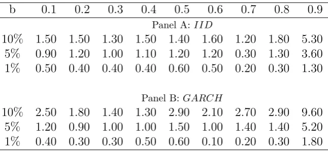
INSERT TABLE 1 HERE
INSERT TABLE 2 HERE
Tables 1 and 2 report the rejection rates of the tests at the 10%, 5% and 1% levels.
con-trolling the size. The performance is slightly worst when one of the roots is close to the
unit circle and when we consider the GARCH process.
4
Empirical Application
In order to investigate the performance of the test, I consider the model of Blanchard
and Quah (1989) which represents the origin of the debate on non-fundamentalness. The
equilibrium solution for unemployment rateUt and output growth ∆Ythas the structural
form:
∆Yt
Ut =
1−L d(L) + (1−L)a
−1 −a
ξt,d ξt,s (4.1)
BQ assume no dynamics in productivity except for the instantaneous response to the
supply shock, i.e., d(L) = 1. This assumption implies that the determinant of the MA polynomial equals to unity and the model is invertible. Lippi and Reichlin (1993),
how-ever, argue that economic theory does not provide sufficient conditions on the roots of
d(L) and the invertibility of (4.1) is not automatically guaranteed.
I now apply the test to empirically evaluate the validity of the invertibility assumption
of the model (4.1). The quarterly time series data is obtained from the St. Louis Fed
website, using the seasonally adjusted series GNPC96 and UNRATE. Here, I extend the
sample to cover the period 1948:1 to 2010:4 as opposed to the period 1948:1-1989:4 in
the original paper.
Following BQ, I estimate a bivariate VAR system in real GNP growth and
unem-ployment rate, allowing for eight lags and obtain the residuals, ˆξt, which is the inputs of
our test. Since the test relies on a non-Gausianity assumption of the estimated
residu-als, I first provide some empirical evidence of it. We reject the null of normality in the
5
Conclusions
This paper provides a new testing procedure to empirically detect fundamentalness,
con-vert the fundamentalness testing problem into one of predictability of the Wold
innova-tions. The proposed test is simple to apply since it only needs model residuals and fitted
values as input and can be implemented using a simple F-test. The test is robust to the
conditional heteroskedasticity of unknown form and does not need information outside of
the specified model. The Monte Carlo study based on a DSGE model with fiscal foresight
Table 1: Size Performance
b 0.1 0.2 0.3 0.4 0.5 0.6 0.7 0.8 0.9
Panel A:I I D
10% 1.50 1.50 1.30 1.50 1.40 1.60 1.20 1.80 5.30 5% 0.90 1.20 1.00 1.10 1.20 1.20 0.30 1.30 3.60 1% 0.50 0.40 0.40 0.40 0.60 0.50 0.20 0.30 1.30
Panel B:GARCH
10% 2.50 1.80 1.40 1.30 2.90 2.10 2.70 2.90 9.60 5% 1.20 0.90 1.00 1.00 1.50 1.00 1.40 1.40 5.20 1% 0.40 0.30 0.30 0.50 0.60 0.10 0.20 0.30 1.80
[image:9.595.138.461.94.243.2]Notes: Percentage of rejections across 1000 experiments for the null of fundamental-ness of the VAR with 4. Sample size is 200.
Table 2: Power Performance
b 2 3 4 5 6 7 8 9 10
Panel A:I I D
10% 92.7 99.8 99.9 100 99.7 98.8 97.9 95.9 91.4 5% 89.9 99.6 99.9 100 99.5 98.2 97.0 94.3 88.4 1% 80.5 98.5 99.9 100 98.6 96.2 93.4 88.6 79.3
Panel B:GARCH
10% 63.3 85.4 90.7 95.0 95.1 93.3 89.5 86.9 83.7 5% 57.6 81.9 88.8 92.3 93.1 90.2 84.8 80.7 77.4 1% 47.9 76.2 84.1 87.0 87.0 81.7 74.0 67.5 62.5
References
Bierens, H. J., 1990. A consistent conditional moment test of functional form.
Econo-metrica: Journal of the Econometric Society, pages 1443–1458.
Blanchard, O. J. and Quah, D., 1989. The Dynamic Effects of Aggregate Demand and
Supply Disturbances. American Economic Review, 79(4):655–73.
Hamidi Sahneh, M., 2014. Are the shocks obtained from svar fundamental? URL
https://editorialexpress.com/cgi- bin/conference/download.cgi?db_name=
EWM2014&paper_id=170.
Leeper, E. M., Walker, T. B., and Yang, S.-C. S., 2013. Fiscal foresight and information
flows. Econometrica, 81(3):1115–1145.
Lippi, M. and Reichlin, L., 1993. The dynamic effects of aggregate demand and supply
disturbances: reply. The American Economic Review, 83(0):653–658.
Lippi, M. and Reichlin, L., 1994. Var analysis, nonfundamental representations, blaschke
matrices. Journal of Econometrics, 63(1):307–325.
Stinchcombe, M. B. and White, H., 1998. Consistent specification testing with nuisance