Computer Simulation of Multiphase Binary Diffusion in Gas Solid Type Couples

(1)

Computer Simulation of Multiphase Binary Diﬀusion in Gas–Solid Type Couples

Shinji Tsuji

Department of Mechanical and Precision System, School of Science and Engineering, Teikyo University, Utsunomiya 320-8551, Japan

Model 1 for describing multiphase diffusion and Model 2 for determining the interdiffusion coefficient of each phase in binary gas–solid couples were developed by modifying models previously presented. No restrictions on the number of phases, the values of interdiffusion coefficients, or the homogeneity ranges of phases were placed on the present models.

Composition profiles, mass changes per unit area of surface and dimensional changes normal to the surface for N–Cr, N–Fe, and N–Ti couples were numerically calculated from diffusivity and phase equilibrium data with Model 1. A good agreement between experimental and calculated results was found. It was confirmed that Model 1 is compatible with Model 2, which can be easily applied and is useful when no references are available for diffusivity data.

(Received December 9, 2004; Accepted April 20, 2005; Published June 15, 2005)

Keywords: computer simulation, composition profile, mass change, dimensional change, layer width, interdiffusion coefficient, phase boundary composition, partial molar volume, nitriding, nitrogen–chromium system, nitrogen–iron system, nitrogen–titanium system

1. Introduction

In binary gas–solid couples, new phases often form as layers parallel to the surface. For example, if pure iron is oxidized, Fe2O3, Fe3O4and FeO form on the surface under given conditions. Similar behavior is observed during case hardening processes such as carburizing and diffusion coat-ing processes such as chromizcoat-ing. Estimation of the layer width and simulation of the composition profile in the diffusion zone at any diffusion time are interesting, not only from a theoretical but also from a practical point of view.

An analytical solution for two-phase diﬀusion in a binary semi-inﬁnite medium was presented by Jost,1)_{but no solution}

has been derived for more than one product phase. Ja¨ger and Matauschek2)_{presented approximate solutions for the layer}

growth of one and two product phases in a semi-infinite medium on the assumption of the linear concentration in a phase. The solutions can be easily generalized to a general n-phase system. However, their method is not totally satisfac-tory because it gives no description of the composition profiles. Two different models, for describing multiphase diffusion3) (Model 1) and determining the interdiffusion coefficient in each phase4) (Model 2) were developed for Boltzmann–Matano type diffusion where a variable

x=t1=2_{is introduced and the solution}_c

i¼ciðÞis assumed.

It has already been pointed out5)_{that the layer growth rate}

of a product phase increases proportionally to the product of the square root of the interdiffusion coefficient and the homogeneity range of the phase, if the miscibility gap between adjacent phases is excluded. Therefore, a rise in the number of phases present in a couple and a drop in the amount of the preceding product make the simulation still more difficult. One purpose of the present study was to develop a general model for the numerical description of binary multiphase diffusion without being restricted by the number of phases, the interdiffusion coefficient, or the homogeneity range of a phase. This was done by modifying the preceding Model 1.

Equilibrium phase boundary data and diﬀusion data are

needed to execute Model 1. The former data are available for almost all binary systems (for example, reference6)_{). The}

latter data are available for some limited systems only. It is therefore useful to apply Model 2 to systems for which there are no available diﬀusivity data. Another purpose of the present study is to verify the compatibility between Models 1 and 2.

2. Models

For general gas–solid binary couples, one diﬀusing component, A, is transferred from the gas phase to the solid phase, and the other component, B, is transferred in the opposite direction. The following assumptions are made:

(a) the composition at each phase boundary, including that at the surface, is time independent;

(b) the interdiﬀusion coeﬃcient in each phase, DðjÞ, is composition independent;

(c) the ratio of the number of moles for component A entering the solid phase to that for componentBleaving the solid phase,, is time independent.

In gas–solid couples, for such diffusion processes as nitriding and carburizing, the partial molar volume of the diffusing gas component, A, is much smaller than that of the metallic diffusing component, B. However, most analyses of diffusion in gas–solid couples have ignored possible effects due to variations of molar volume with composition, and have assumed constant molar volume over the composition range considered. Nevertheless, these effects should be of significance in the calculated composition profile, mass change, and dimensional change of the solid phase. The additional assumption is made here that:

(d) molar volume changes linearly with composition. The present numerical simulation of multiphase diﬀusion in gas–solid couples consists of the following two models:

(1) numerical calculation for describing the Boltzmann– Matano type of diﬀusion where the concentration of a diﬀusing component, c, can be expressed in terms of a single variablex=t1=2;

(2)

(2) numerical calculation of the interdiffusion coefficient for each phase in the Boltzmann–Matano type of diffusion couple.

2.1 Numerical calculation for describing multiphase diﬀusion (Model 1)

The equations describing the concentration proﬁles in the product phase jand the terminal phasenare given by

cA¼CAðj;j1Þ þ

CAðj;jþ1Þ CAðj;j1Þ

erf½!ðj;jþ1Þ erf½!ðj;jiÞ ferf½ erf½!ðj;j1Þg ð1Þ

and

cA¼CAðn;nþ1Þ

CAðn;nþ1Þ CAðn;n1Þ

1erf½!ðn;n1Þ

f1erf½g ð2Þ

where¼x=½2t1=2_D_ð_j_Þ1=2

¼=½2DðjÞ1=2,CAðj;j1Þ ¼

NAðj;j1Þ=fNAðj;j1Þ VAþ ½1NAðj;j1Þ VBg. The

termVistands for the partial molar volume of componenti,

NAðj;j1Þstands for the mole fraction of componentAat

the phase boundary in phasejcoexisting with phasej1or jþ1,NAð1;0Þstands for that at the surface; andNAðn;nþ1Þ

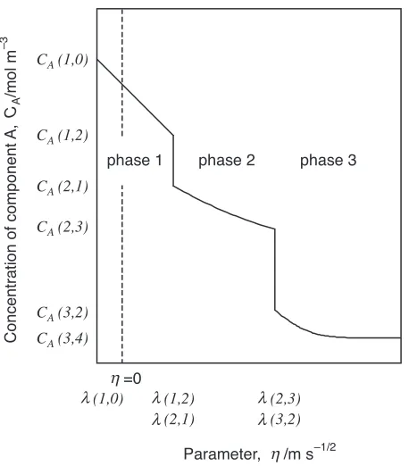
stands for that in the solid phase att¼0. An example of a schematiccAproﬁle is shown in Fig. 1.

The unknowns !ðj;j1Þ, where j¼1;2;. . .;n, can substantially be obtained by a binary bisection method.3) By adding a modification, a general numerical method that is not restricted by the number of phases present in the couple, the interdiffusion coefficient and the solubility range of a phase has been developed. Provided that the parameters !ðj;j1Þare all known, the following characteristic values can be obtained:

ðj;j1Þ the rate constant for the moving of interfaces

ðj1=jÞ or ðj=jþ1Þ[ms1=2_{] =}₂_!_ð_j;_j₁_Þ DðjÞ1=2;

Xðj;j1Þ the displacement of interface ðj1=jÞ or

ðj=jþ1Þ relative to the x¼0 plane [m] = t1=2_ð_j;_j₁_Þ_;

XS the displacement of the surface relative to the

x¼0plane [m] =Xð1;0Þ;

kWðjÞ the rate constant for layer growth of phase j[ms1=2_{] =}_ð_j;_j_þ₁_Þ_ð_j;_j₁_Þ_;

WðjÞ the layer width of phase j[m] =Xðj;jþ1Þ

Xðj;j1Þ;

PðjÞ[x;NA] the point expressed by the distance and mole

fraction of componentA;

kM the rate constant for mass change per unit area of surface [gm2s1=2];

M the change in mass of the solid phase per unit area of surface [gm2_{] =}_t1=2_kM_.

kM is given by the following equation which eq. (27) in Ref. 3) has been modiﬁed into:

kM¼ ð1;0Þ Að1;0Þ ðRAþRBÞ ð3Þ

where

Að1;0Þ ¼1=ðVAþVBÞ ð4Þ

andRiin eq. (3) is the relative atomic mass of component i.

The data necessary for the calculation and some character-istic calculated data are shown in Fig. 2.

2.2 Numerical calculation of interdiﬀusion coeﬃcients (Model 2)

We developed a model for determining interdiﬀusion coeﬃcients for all the phases present in a gas–solid couple.4)

With this model there is no need to evaluate the concentration gradient in each phase. The method principally consists of the calculation of integrals and determination of XS by the

following equations, respectively:

SiðjÞ ¼

Z Xðj;jþ1Þ

Xðj;j1Þ

½ciCiðn;nþ1Þdx ð5Þ

and

phase 1 phase 2 C_A (1,0)

C_A (1,2)

C_A (2,1)

C_A (2,3)

C_A (3,2) C_A (3,4)

(1,0) (1,2) λ

λ η λ

λ λ

(2,3)

Concentration of component

A,

CA

/mol m

–3

Parameter, /m s–1/2

(2,1) (3,2)

phase 3

=0

η

Fig. 1 Schematic–c proﬁle of three-phase diﬀusion in a gas–solid couple.

D (j)

NA(j, j 1)

VA, VB RA, RB

γ

(j, j 1)

ω

λ(j, j 1) kW (j) kM

P(j)(x,NA) XS W(j)

M

∆

t

Fig. 2 Input and output data used in Model 1. Here,PðjÞ½x;NAdenotes a

[image:2.595.57.286.494.755.2] [image:2.595.308.543.522.736.2]

(3)

Xs¼

RA

Xn

k¼1

SAðkÞ þRB

Xn

k¼1

SBðkÞ M

RACAðn;nþ1Þ þRBCBðn;nþ1Þ

ð6Þ

Here,Mcan be obtained, provided thatXSis known. From

eqs. (17a, b) in Ref. 3) and eq. (44) in Ref. 4), the mole ratio is given by

¼

Xn

k¼1

SBðkÞ CBðn;nþ1Þ XS

Xn

k¼1

SAðkÞ CAðn;nþ1Þ XS

ð7Þ

The number in moles of componentihaving passed through interfaceðj=jþ1Þis given by

Qiðj=jþ1Þ ¼

Xn

k¼jþ1

SiðkÞ Ciðn;nþ1Þ Xðj;jþ1Þ ð8Þ

Now, we can numerically calculate interdiﬀusion coeﬃcients for all the phases present by the initial substitution of QAðj=jþ1ÞandQBðj=jþ1Þand the sequential substitution

of the results obtained into the following equations,3)_i.e.

ðj=jþ1Þ ¼QAðj=jþ1Þ=QBðj=jþ1Þ ð9Þ

Aðj;jþ1Þ ¼Aðjþ1;jÞ

¼ðj=jþ1Þ=½ðj=jþ1ÞVAþVB ð10Þ

exp Xðj;jþ1Þ

2_X_ð_j;_j₁_Þ2

4DðjÞ t

¼Xðj;j1Þ ½Aðj;j1Þ CAðj;j1Þ

Xðj;jþ1Þ ½Aðj;jþ1Þ CAðj;jþ1Þ

ð11aÞ

and

f Xðn;n1Þ 2½DðnÞ t1=2

¼CAðn;nþ1Þ CAðn;n1Þ

Aðn;n1Þ CAðn;n1Þ

ð11bÞ

wherefð!Þ ¼1=2_!_erfc_ð_!_Þ_exp_ð_!2_Þ_.

The necessary data for the calculation and some character-istic calculated data are shown in Fig. 3.

3. Example of Simulations

Nitriding of chromium, iron, and titanium will be used as examples here since equilibrium and diﬀusivity data are

available as input data for their systems, and the reliable mass changes, dimensional changes and diffusion layer widths needed for comparison with the calculated results have been measured. It is possible by either Model 1 or Model 2 to make simulations of composition profiles and the associated changes, provided that the equilibrium and diffusivity or experimental data are known.

By approximating the linear dependence of molar volumes on composition, the partial molar volumes of both the diﬀusing components for a given system were calculated from the molar volumes of nitrides and the parent pure metal in reference to the lattice parameter data.7)Phase boundary compositions excluding the surface composition were taken from the equilibrium phase diagrams.6)

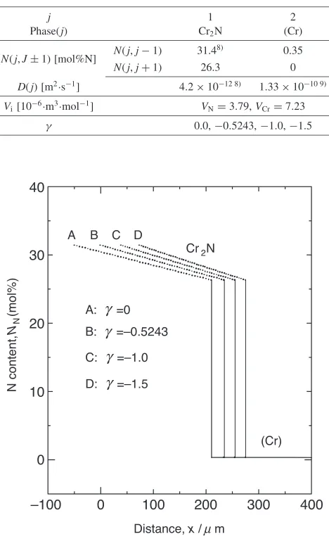
3.1 Nitriding of Chromium

Nitrogen content proﬁles of nitrided chromium calculated from Table 1 are shown in Fig. 4. The proﬁle for case A stands for expansion normal to the surface, that for case B no change, and those for C and D, shrinkage. On the other hand, the following equations were already deduced in Ref. 3),i.e.

NA(j, j 1)

W(j) P(j)[x, NA] VA, VB RA, RB t

M or X

∆ S

D(j)

(j, j 1)

P(j)[x, NA] γ

λ ω

XS or ∆M

Fig. 3 Input and output data used in Model 2. Here,PðjÞ½x;NAmust be

input when a linear approximation is not made of the composition proﬁle in phasej. The bottom item on the left side means thatXSis output in the

[image:3.595.49.296.349.523.2]

case whereMis input, andMis output in the case whereXSis input.

Table 1 Phase boundary compositions, interdiﬀusion coeﬃcients, partial molar volumes, and the mole ratio for the N–Cr system at 1473 K utilized in the calculations using Model 1.

j Phase(j)

1 Cr2N

2 (Cr)

Nðj;J1Þ[mol%N] Nðj;j1Þ 31.4

8Þ _0.35

Nðj;jþ1Þ 26.3 0 DðjÞ[m2_s1_] ₄_:₂₁₀12 8Þ ₁_:₃₃₁₀10 9Þ

Vi[106m3mol1] VN¼3:79,VCr¼7:23

0.0,0:5243,1:0,1:5

–100 0 100 200 300 400 0

10 20 30 40

N content,

NN

(mol%)

Distance, x /

A B C D

A: γ =0 B: =–0.5243 C: =–1.0 D: =–1.5

Cr₂N

(Cr)

m µ

γ γ γ

[image:3.595.310.544.376.759.2] [image:3.595.56.284.625.735.2]

(4)

1=2!ð1;0Þferf½!ð1;0Þ !ð1;2Þg exp½!ð1;0Þ2

¼CAð1;0Þ CAð1;2Þ

Að1;0Þ CAð1;0Þ

ð12Þ

When takes the value of case B, it makes the termVAþ

VB nearly equal to zero, and then the parameter Að1;0Þ

approaches inﬁnity, as is clear from eq. (4). Next, when Að1;0Þhaving the value of inﬁnity is substituted into eq. (3), i.e.

XS¼

M Að1;0Þ ðRAþRBÞ

ð13Þ

it can be seen that!ð1;0Þwhich is written asXS=½2Dð1Þt1=2

becomes nearly zero. Equation (1), where j¼1, therefore, yields

cA¼CAð1;0Þ þ

CAð1;2Þ CAð1;0Þ

erf½!ð1;2Þ

erff=½2Dð1Þ1=2g ð14Þ

Equation (14) is identical to the solution1)_{to diﬀusion into a}

homogeneous phase, a second phase developing from the surface given by Jost. That is, it is apparent that the solution by Jost can be applied only to no net transfer of volume through the surface for both diﬀusing components. Figure 4 shows that Xs increases from a negative value to a larger

positive value with a decrease in mole ratio , that is, the dimensional change of the nitrided chromium normal to the surface continuously varies from expansion to shrinkage with a decrease in.

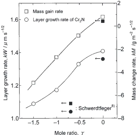
The dependence of the rate constant for layer growth of Cr2N and the rate constant for mass change upon the mole ratio are shown in Fig. 5, in which both of them decrease with a decrease in and especially the latter reaches negative values. An ammonia gas used in gas nitriding processes is decomposed into nascent nitrogen and hydrogen at the nitriding temperature,i.e.

NH3!Nþ3H

For example, the nascent nitrogen reacts with chromium and forms chromium nitride. It is clear from the above reaction equation that the mole ratio is zero when the evaporation rate of chromium from the surface is negligibly small. Therefore, the nitriding processes will not result in the mass losses seen in Cases B, C, and D. On the other hand, in siliconizing processes performed on iron with silicon tetra-chloride under neutral atmosphere, the following substitution reaction mainly occurs:

SiCl4(g)þ2Fe(s)¼Si(in Fe)þ2FeCl2

where the mole ratio has the value-2. It has been reported by Mitani and Onishi10) that the mass loss of siliconized steel decreases parabolically with treatment time. Their observa-tions correspond to the negative value of the mole ratio.

The experimental values ofkW(Cr2N) andkMobtained by Schwerdtfeger8) _{are less than the calculations in the case}

where¼0. This is perhaps due to evaporation of chromium at the high nitriding temperature 1473 K employed in his study. Even if this is not so, the calculations show close agreement with the experimental results.

3.2 Nitriding of Iron

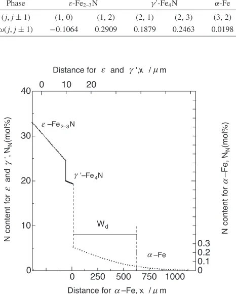
The parameters !ðj;j1Þ, calculated from the data in Table 2 are shown in Table 3. Substituting !ð1;0Þ and !ð1;2Þfor the most outer product phase"-Fe2{3N,!ð2;1Þand !ð2;3Þfor the inner product phase0-Fe4N into eq. (1), and !ð3;2Þfor the terminal phase-Fe into eq. (2) gives acA–

curve or a NA–x curve. The nitrogen content proﬁle thus

calculated is shown in Fig. 6. As is clear from the ﬁgure, the -Fe layer in which nitrogen atoms diﬀuse away is much wider than the compound layer, which consists of"-Fe2{3N

Fig. 5 Dependence of mass change rate and layer growth rate on for chromium nitrided at 1473 K. The arrow indicates that a negative value of

[image:4.595.311.541.72.299.2]

is possible.

Table 2 Phase boundary compositions, interdiﬀusion coeﬃcients, partial molar volumes, and the mole ratiofor the N–Fe system at 773 K utilized in the calculations using Model 1.

j Phase(j)

1

"-Fe2{3N

2

0_-Fe 4N

3

-Fe

Nðj;J1Þ[mol%N] Nðj;j1Þ 33 20 0.26

11Þ

Nðj;jþ1Þ 24.6 19.3 0

DðjÞ[m2_s1_] ₉_:₈₁₀15 12Þ ₂_:₃₅₁₀14 13Þ ₃_:₆₅₁₀12 14Þ

Vi[106m3mol1] VN¼4:24,VFe¼7:04

[image:4.595.52.549.691.785.2]

(5)

and0_-Fe

4N. The width of the diﬀusion layer,Wd, is deﬁned

as the distance from the0_-Fe

4N/-Fe interface to the plane at which-Fe is saturated with 0.046 mol% N at 573 K. The calculated diﬀusion layer width of 616mmagrees well with the experimental result15)_{of about 650}_m_m_.

Steel parts increase slightly in size during nitriding. This dimensional change is aﬀected by such factors as the temperature and time of nitriding, the relative thicknesses of the nitriding layer and core, and the shape of the parts. An expansion of the order of a 40mmincrease in diameter occurs in solid round bars made of Nitralloy 135 nitrided at 798 K for 259.2 ks.16) _{On the other hand, calculations with the}

diﬀusivity and equilibrium data for the N–Fe system under the preceding heating conditions result in expansion of 28.5mmin diameter. Nitralloy 135 containing such alloying components as aluminum, chromium, and molybdenum with higher aﬃnity for nitrogen than iron will take in a greater mass of nitrogen; furthermore, the partial molar volume of nitrogen for "-Fe2{3N is 12:4106m3/mol,17) which is much larger than that in Table 2. This leads to greater expansion in diameter for the Nitralloy 135, as is clear from the following equation, which is obtained from the combi-nation of eq. (4) with eq. (13) for the condition¼0:

XS¼

MVA

RA

ð15Þ

Therefore, provided that these eﬀects are taken into consid-eration, the expansion calculated will be larger, and the diﬀerence between the calculated and experimental results will become a reasonable value.

3.3 Nitriding of Titanium

[image:5.595.47.289.85.135.2]

ThekWðjÞ,kM, andð1;0Þcalculated from the data shown in Table 4 and those experimentally obtained, are shown in Table 5. As can be seen in the table, the agreement between the calculated and experimental results in terms of both quantities is quite satisfactory. The layer growth rates calculated for "-Ti2N and -Ti are larger than those experimentally obtained, for which ion nitriding was em-ployed. It is generally known that layer growth rates are larger for ion nitriding than for gas nitriding. Figure 7 shows

Table 3 Values of!ðj;j1Þcalculated from data given in Table 2. j

Phase

1

"-Fe2{3N

2

0_-Fe4N

3

-Fe

ðj;j1Þ (1, 0) (1, 2) (2, 1) (2, 3) (3, 2)

!ðj;j1Þ 0:1064 0.2909 0.1879 0.2463 0.0198

0 250 500 750 1000

0 10 20 30

40 0 10 20

0 0.1 0.2 0.3 –Fe2–3N

ε

γ

α

'–Fe4N

–Fe

N content for

εγ

and

',

NN

(mol%)

N content for

α

–Fe,

NN

(mol%)

Distance for –Fe, x

W_d

µ

α / m

Distance for ε and γ',x /µm

[image:5.595.54.287.99.389.2]

Fig. 6 Calculated nitrogen content proﬁle in iron nitrided at 773 K for 28.8 ks.

Table 4 Phase boundary compositions, interdiﬀusion coeﬃcients, partial molar volumes, and the mole ratiofor the N–Ti system at 1173 K utilized in the calculations using Model 1.

j Phase(j)

1 -TiN

2

"-Ti2N

3

-Ti

4

-Ti

Nðj;J1Þ[mol%N] Nðj;j1Þ 51.2

18Þ _33.8 _15.5 _0.14

Nðj;jþ1Þ 38.1 32.8 1.2 0.0

DðjÞ[m2_s1_] ₁_:₁₁₁₀16 19Þ ₈_:₀₄₁₀16 20Þ ₄_:₀₉₁₀15 19Þ ₁_:₇₇₁₀12 19Þ

Vi[106m3mol1] VN¼0:80,VTi¼10:8

[image:5.595.43.553.550.645.2]

0

Table 5 Comparison of calculated rate constants for layer growth of phase j and mass gain per unit area of surface with those experimentally obtained for titanium nitrided at 1173 K.

Product phase Rate constant

1: -TiN 2:"-Ti2N 3:-Ti

kWðjÞ[ms1=2_] Calculated values 5:0610

9 ₂_:₀₉₁₀9 ₁_:₄₂₁₀7

Experimental values 2:54108 18Þ ₁_:₆₂₁₀7 18Þ

kM[gm2_s1=2_] Calculated values 2:3710

2

Experimental values 1:96102 21Þ_,₁_:₇₇₁₀2 22Þ

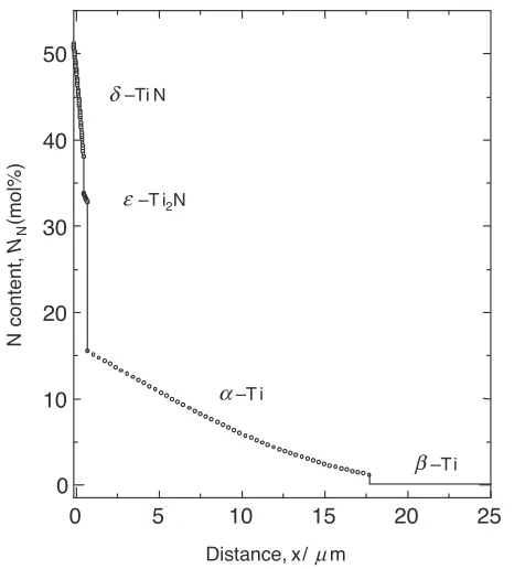
[image:5.595.55.548.690.785.2]

(6)

a nitrogen content proﬁle calculated from the values in Table 4. Although the proﬁle in-Ti seems parallel to thex -axis, a decrease in nitrogen content from 0.14 to 0.01 mol% N extends over 413mm.

The quantitiesWðjÞ,PðjÞ½x;NA,SiðjÞandM shown in

Table 6, which had been calculated from the data in Table 4, were utilized for determination of the interdiﬀusion coef-ﬁcients of the phases using Model 2. Here, the following two cases are dealt with:

Case 1, nitrogen content proﬁles in -TiN and"-Ti2N were assumed to be linear;

Case 2, those in -TiN,"-Ti2N and-Ti were to be linear. In the case where a nitrogen content proﬁle is approximated by a linear function,SiðjÞis given by

SiðjÞ ¼WðjÞ ½Ciðj;j1Þ þCiðj;jþ1Þ=2 ð16Þ

In the case where a nitrogen content proﬁle is described by PðjÞ½x;NA,SiðjÞwas evaluated using the Simpson

integra-tion formula. UsingSiðjÞ thus obtained,XScalculated from

eq. (6), from eq. (7), andDðjÞfrom eqs. (8), (9), (10), and (11a, 11b) are shown in Table 7 together. Here, DðjÞ ¼

100 ½D_ð_j_Þ_D_ð_j_Þ_=D_ð_j_Þ_{, where}_D_ð_j_Þ_{stands for}_D_ð_j_Þ_in

Table 4 andDðjÞstands for that calculated from eqs. (11a) and (11b) in Model 2. To obtain a more accurate interdiffu-sion coefficient it is necessary to input data closer to the original concentration profile, as clear from a comparison of Cases 1 and 2 in Table 7. Using the closer input data also gives more accurate and XS, as is understood from a

comparison of in Table 4 and S (¼XS=t1=2) in Table 5

with those in Table 7. The above shows that Model 1 and Model 2 are compatible with no inconsistencies between them.

0 5 10 15 20 25 0

10 20 30 40 50

δ

ε

β α

–Ti N

–T i₂N

–T i

N content,

NN

(mol%)

Distance, x/µm

[image:6.595.54.292.69.327.2]

Fig. 7 Calculated nitrogen content proﬁle in titanium nitrided at 1173 K for 14.4 ks.

Table 6 Layer widths, points as a function of distance and nitrogen content, and mass gain per unit area of surface calculated from the values in Table 4 using Model 1. Here, distancexis measured relative to the interfaceðj1=jÞ. Temperature and time for nitriding are 1173 K and 14.4 ks, respectively.

j Phase

1 -TiN

2

"-Ti2N 3

-Ti

4

-Ti

WðjÞ[mm] 0.6 0.25 16.99 463.2

1.7, 13.66 48.3, 0.12 3.4, 11.80 96.5, 0.09 5.1, 9.99 144.7, 0.07 6.8, 8.25 193.0, 0.05 PðjÞ½x;NA[mm, mol% N] 8.5, 6.65 241.2, 0.04

10.2, 5.19 289.5, 0.03 11.9, 3.92 337.7, 0.02 13.6, 2.83 386.0, 0.01 15.3, 1.93 434.2, 0.01

[image:6.595.306.551.122.285.2]

M[gm2_] _2.85

Table 7 IntegrationSiðjÞobtained from the values in Table 6, and dimensional change normal to the surfaceXS, the mole ratio ofand

interdiﬀusion coeﬃcients that were calculated using Model 2.

j Phase

1 -TiN

2

"-Ti2N

3

-Ti

4

-Ti

SNðjÞ[molm2] 4:34102 1:12102 1:519101 2:27102

STiðjÞ[molm2] 3:21103 8:3104 1:125102 1:68103

Case 1 Xs[mm] 0:10

0:033

DðjÞ[m2_s1_] ₁_:₂₈₁₀16 ₉_:₂₉₁₀16 ₃_:₆₉₁₀15 ₁_:₈₀₁₀12

DðjÞ[%] 15.3 15.5 9:8 1.7

SNðjÞ[molm2] 4:34102 1:12102 1:256101 2:27102

STiðjÞ[molm2] 3:21103 8:3104 9:30103 1:68103

Case 2 Xs[mm] 0:16

0.001

DðjÞ[m2_s1_] ₁_:₁₀₁₀16 ₇_:₉₉₁₀16 ₄_:₀₁₁₀15 ₁_:₇₉₁₀12

[image:6.595.45.552.600.786.2]

(7)

4. Conclusions

Model 1 for describing multiphase diffusion and Model 2 for determining interdiffusion coefficients for each phase present in binary gas–solid couples have been developed by modifying the models previously presented. It has been confirmed that Model 1 is compatible with Model 2. No restriction is imposed on the number of phases, the interdiffusion coefficients, or the homogeneity ranges of phases.

The good agreements between the numerical and exper-imental results shows that Model 1 is capable of predicting composition proﬁles, mass changes per unit area of surface, and dimensional changes normal to the surface. It is apparent that Model 2 can be easily applied, and is useful when no references are available for diﬀusivity data.

REFERENCES

1) W. Jost:Diﬀusion in Solids, Liquids and Gases, (Academic Press, New York, 1960) pp. 71–72.

2) I. Ja¨ger and Matauschek: Z. Metallkd.69(1978) 761–765. 3) S. Tsuji: Metall. Mater. Trans. A25A(1994) 753–761. 4) S. Tsuji: Metall. Mater. Trans. A25A(1994) 741–751. 5) S. Tsuji: J. Jpn. Inst. Met.41(1977) 678–685.

6) T. B. Massalski:Binary Alloy Phase Diagrams, (ASM, Ohio, 1986). 7) P. Villars and L. D. Calvert:Pearson’s Handbook of Crystallographic

Data for Intermetallic Phases, (The Materials Information Society, Ohio, 1991).

8) K. Schwerdtfeger: Trans. AIME239(1967) 1432–1438. 9) M. J. Klein: J. Appl. Phys.38(1967) 167–170.

10) Y. Mitani and M. Onishi: J. Jpn. Inst. Met.23(1959) 273–276. 11) R. Rawlings and D. Tambini: J. Iron Steel Inst.184(1956) 302. 12) M. O. Speidel: Proc. 2nd High Nitrogen Steels (Aachen 1990) 128. 13) G. E. Totten and M. A. H. Howes:Steel Heat Treatment Handbook,

(Marcel Dekker Inc., 1997) p. 695.

14) J. D. Fast and M. B. Verrijp: J. Iron Steel Inst.176(1954) 24. 15) T. Sone, E. Tsunasawa and K. Yamanaka: Netsu Shori24(1984) 316–

322.

16) American Society for Metals:Metals Handbook 9th Ed., vol. 4, (ASM,

Ohio, 1980) pp. 199–203.

17) V. G. Paranjpe, M. Cohen, M. B. Bever and C. F. Floe: Trans. AIME, 188(1950) 261–267.

18) E. Metin and O. T. Inal: Metall. Trans. A20A(1989) 1819–1832. 19) R. J. Wasilewski and G. L. Kehl: J. Inst. Metals.83(1954) 94–104. 20) F. W. Wood and O. G. Paasche: Thin Solid Films40(1977) 131–137. 21) L. S. Richardson and N. J. Grant: Trans. AIME200(1954) 69–70. 22) Yu. V. Levinskii: Izv. Akad Nauk SSSR Neorg Mater.4(1968) 2068–

2073.

Appendix

Almost all the symbols in this paper correspond to those used in the previous papers.3,4)The parameter!ðj;j1Þand the rate constantsðj;j1Þ, as an example, in Refs. 3) and 4) were written as

ðj;j1Þ ¼!ðj;j1Þ DðjÞ1=2 ðA:1Þ

and

Xðj;j1Þ ¼ðj;j1Þ 2t1=2 ðA:2Þ

Those in this paper, however, are deﬁned as

ðj;j1Þ ¼!ðj;j1Þ 2DðjÞ1=2 ðA:3Þ

and

Xðj;j1Þ ¼ðj;j1Þ t1=2 ðA:4Þ

In eq. (23) in Ref. 3), which is written as

dQAð0=1Þ

dt ¼ Dð1Þ @cA

@x

S