Application Note 150
Agilent
2
Contents
Chapter 1
Introduction ...3
What is a spectrum? ...3
Why measure spectra? ...4
Chapter 2 The superheterodyne spectrum analyzer...6
Tuning equation ...8
Resolution...11
Analog filters ...11
Digital filters ...13
Residual FM ...14
Phase noise ...14
Sweep time...15
Analog resolution filters...15
Digital resolution filters ...16
Envelope detector...17
Display smoothing...18
Video filtering...18
Video averaging ...20
Amplitude measurements...21
CRT displays...21
Digital displays...22
Amplitude accuracy...25
Relative uncertainty ...25
Absolute accuracy ...26
Improving overall uncertainty ...26
Sensitivity ...27
Noise figure...29
Preamplifiers ...30
Noise as a signal ...33
Preamplifier for noise measurements ...35
Dynamic range...36
Definition ...36
Dynamic range versus internal distortion ...36
Attenuator test ...39
Noise ...39
Dynamic range versus measurement uncertainty...40
Mixer compression ...41
Display range and measurement range...42
Frequency measurements ...42
Summary...43
Chapter 3 Extending the frequency range ...44
Harmonic mixing ...44
Amplitude calibration ...47
Phase noise ...48
Signal identification ...48
Preselection ...50
Improved dynamic range ...51
Multiband tuning ...52
Pluses and minuses of preselection...53
Wideband fundamental mixing ...53
Summary...55
Glossary of terms ...56
Index ...63
3
Chapter 1
Introduction
This application note is intended to serve as a primer on superheterodyne spectrum analyzers. Such analyzers can also be described as frequency-selective, peak-responding voltmeters calibrated to display the rms value of a sine wave. It is impor-tant to understand that the spectrum analyzer is not a power meter, although we normally use it to display power directly. But as long as we know some value of a sine wave (for example, peak or average) and know the resistance across which we measure this value, we can calibrate our voltmeter to indicate power.
What is a spectrum?
Before we get into the details of describing a spec-trum analyzer, we might first ask ourselves: just what is a spectrum and why would we want to analyze it?
Our normal frame of reference is time. We note when certain events occur. This holds for electrical events, and we can use an oscilloscope to view the instantaneous value of a particular electrical event (or some other event converted to volts through an appropriate transducer) as a function of time; that is, to view the waveform of a signal in the time domain.
Enter Fourier.1He tells us that any time-domain electrical phenomenon is made up of one or more sine waves of appropriate frequency, amplitude, and phase. Thus with proper filtering we can decompose the waveform of figure 1 into separate sine waves, or spectral components, that we can then evaluate independently. Each sine wave is characterized by an amplitude and a phase. In other words, we can transform a time-domain sig-nal into its frequency-domain equivalent. In gener-al, for RF and microwave signals, preserving the phase information complicates this transformation process without adding significantly to the value of the analysis. Therefore, we are willing to do with-out the phase information. If the signal that we wish to analyze is periodic, as in our case here, Fourier says that the constituent sine waves are separated in the frequency domain by 1/T, where T is the period of the signal.2
To properly make the transformation from the time to the frequency domain, the signal must be evaluated over all time, that is, over ± infinity. However, we normally take a shorter, more practi-cal view and assume that signal behavior over sev-eral seconds or minutes is indicative of the ovsev-erall characteristics of the signal. The transformation can also be made from the frequency to the time domain, according to Fourier. This case requires the evaluation of all spectral components over fre-quencies to ± infinity, and the phase of the individ-ual components is indeed critical. For example, a square wave transformed to the frequency domain and back again could turn into a saw tooth wave if phase were not preserved.
Figure 1. Complex time-domain signal
1 Jean Baptiste Joseph Fourier, 1768-1830, French mathematician and physicist.
4
So what is a spectrum in the context of this discus-sion? A collection of sine waves that, when com-bined properly, produce the time-domain signal under examination. Figure 1 shows the waveform of a complex signal. Suppose that we were hoping to see a sine wave. Although the waveform certain-ly shows us that the signal is not a pure sinusoid, it does not give us a definitive indication of the reason why.
Figure 2 shows our complex signal in both the time and frequency domains. The frequency-domain dis-play plots the amplitude versus the frequency of each sine wave in the spectrum. As shown, the spectrum in this case comprises just two sine waves. We now know why our original waveform was not a pure sine wave. It contained a second sine wave, the second harmonic in this case.
Are time-domain measurements out? Not at all. The time domain is better for many measurements, and some can be made only in the time domain. For example, pure time-domain measurements include pulse rise and fall times, overshoot, and ringing.
Figure 2. Relationship between time and frequency domain
Why measure spectra?
5
Spectral occupancy is another important frequen-cy-domain measurement. Modulation on a signal spreads its spectrum, and to prevent interference with adjacent signals, regulatory agencies restrict the spectral bandwidth of various transmissions. Electromagnetic interference (EMI) might also be considered a form of spectral occupancy. Here the concern is that unwanted emissions, either radiat-ed or conductradiat-ed (through the power lines or other interconnecting wires), might impair the operation of other systems. Almost anyone designing or man-ufacturing electrical or electronic products must test for emission levels versus frequency according to one regulation or another.
So frequency-domain measurements do indeed have their place. Figures 3 through 6 illustrate some of these measurements.
Figure 3. Harmonic distortion test
Figure 5. Digital radio signal and mask showing limits of spectral occupancy
Figure 4. Two-tone test on SSB transmitter
6
Chapter 2
The superheterodyne
spectrum analyzer
While we shall concentrate on the superheterodyne spectrum analyzer in this note, there are several other spectrum analyzer architectures. Perhaps the most important non-superheterodyne type is that which digitizes the time-domain signal and then performs a Fast Fourier Transform (FFT) to dis-play the signal in the frequency domain. One advantage of the FFT approach is its ability to characterize single-shot phenomena. Another is that phase as well as magnitude can be measured. However, at the present state of technology, FFT machines do have some limitations relative to the superheterodyne spectrum analyzer, particularly in the areas of frequency range, sensitivity, and dynamic range.
Figure 7. Superheterodyne spectrum analyzer
Figure 7 is a simplified block diagram of a super-heterodyne spectrum analyzer. Heterodyne means to mix - that is, to translate frequency - and super refers to super-audio frequencies, or frequencies above the audio range. Referring to the block dia-gram in figure 7, we see that an input signal passes through a low-pass filter (later we shall see why the filter is here) to a mixer, where it mixes with a signal from the local oscillator (LO). Because the mixer is a non-linear device, its output includes not only the two original signals but also their har-monics and the sums and differences of the origi-nal frequencies and their harmonics. If any of the mixed signals falls within the passband of the intermediate-frequency (IF) filter, it is further processed (amplified and perhaps logged), essen-tially rectified by the envelope detector, digitized (in most current analyzers), and applied to the ver-tical plates of a cathode-ray tube (CRT) to produce a, vertical deflection on the CRT screen (the dis-play). A ramp generator deflects the CRT beam horizontally across the screen from left to right.1 The ramp also tunes the LO so that its frequency changes in proportion to the ramp voltage.
7
If you are familiar with superheterodyne AM radios, the type that receive ordinary AM broad-cast signals, you will note a strong similarity between them and the block diagram of figure 7. The differences are that the output of a spectrum analyzer is the screen of a CRT instead of a speak-er, and the local oscillator is tuned electronically rather than purely by a front-panel knob.
Since the output of a spectrum analyzer is an X-Y display on a CRT screen, let’s see what information we get from it. The display is mapped on a grid (graticule) with ten major horizontal divisions and generally eight or ten major vertical divisions. The horizontal axis is calibrated in frequency that increases linearly from left to right. Setting the fre-quency is usually a two-step process. First we adjust the frequency at the centerline of the gratic-ule with the center frequency control. Then we adjust the frequency range (span) across the full ten divisions with the Frequency Span control. These controls are independent, so if we change the center frequency, we do not alter the frequency span. Some spectrum analyzers allow us to set the start and stop frequencies as an alternative to set-ting center frequency and span. In either case, we can determine the absolute frequency of any signal displayed and the frequency difference between any two signals.
The vertical axis is calibrated in amplitude. Virtually all analyzers offer the choice of a linear scale calibrated in volts or a logarithmic scale cali-brated in dB. (Some analyzers also offer a linear scale calibrated in units of power.) The log scale is used far more often than the linear scale because the log scale has a much wider usable range. The log scale allows signals as far apart in amplitude as 70 to 100 dB (voltage ratios of 3100 to 100,000 and power ratios of 10,000,000 to 10,000,000,000) to be displayed simultaneously. On the other hand, the linear scale is usable for signals differing by no more than 20 to 30 dB (voltage ratios of 10 to 30). In either case, we give the top line of the graticule, the reference level, an absolute value through cali-bration techniques1and use the scaling per divi-sion to assign values to other locations on the graticule. So we can measure either the absolute value of a signal or the amplitude difference between any two signals.
In older spectrum analyzers, the reference level in the log mode could be calibrated in only one set of units. The standard set was usually dBm (dB rela-tive to 1 mW). Only by special request could we get our analyzer calibrated in dBmV or dBuV (dB rela-tive to a millivolt or a microvolt, respecrela-tively). The linear scale was always calibrated in volts. Today’s analyzers have internal microprocessors, and they usually allow us to select any amplitude units (dBm, dBuV, dBmV, or volts) on either the log or the linear scale.
Scale calibration, both frequency and amplitude, is shown either by the settings of physical switches on the front panel or by annotation written onto the display by a microprocessor. Figure 8 shows the display of a typical microprocessor-controlled analyzer.
But now let’s turn our attention back to figure 7.
Figure 8. Typical spectrum analyzer display with control settings
8
Tuning equation
To what frequency is the spectrum analyzer of fig-ure 7 tuned? That depends. Tuning is a function of the center frequency of the IF filter, the frequency range of the LO, and the range of frequencies allowed to reach the mixer from the outside world (allowed to pass through the low-pass filter). Of all the products emerging from the mixer, the two with the greatest amplitudes and therefore the most desirable are those created from the sum of the LO and input signal and from the difference between the LO and input signal. If we can arrange things so that the signal we wish to examine is either above or below the LO frequency by the IF, one of the desired mixing products will fall within the pass-band of the IF filter and be detected to create a vertical deflection on the display.
How do we pick the LO frequency and the IF to create an analyzer with the desired frequency range? Let us assume that we want a tuning range from 0 to 2.9 GHz. What IF should we choose? Suppose we choose 1 GHz. Since this frequency is within our desired tuning range, we could have an input signal at 1 GHz. And since the output of a mixer also includes the original input signals, an input signal at 1 GHz would give us a constant out-put from the mixer at the IF. The 1 GHz signal would thus pass through the system and give us a constant vertical deflection on the display regard-less of the tuning of the LO. The result would be a hole in the frequency range at which we could not properly examine signals because the display deflection would be independent of the LO.
So we shall choose instead an IF above the highest frequency to which we wish to tune. In Agilent spectrum analyzers that tune to 2.9 GHz, the IF chosen is about 3.6 (or 3.9) GHz. Now if we wish to tune from 0 Hz (actually from some low frequency because we cannot view a to 0-Hz signal with this architecture) to 2.9 GHz, over what range must the LO tune? If we start the LO at the IF (LO - IF = 0) and tune it upward from there to 2.9 GHz above the IF, we can cover the tuning range with the LO-minus-IF mixing product. Using this information, we can generate a tuning equation:
fsig= fLO- fIF
where fsig= signal frequency,
fLO= local oscillator frequency, and fIF = intermediate frequency (IF).
If we wanted to determine the LO frequency need-ed to tune the analyzer to a low-, mid-, or high-fre-quency signal (say, 1 kHz, 1.5 GHz, and 2.9 GHz), we would first restate the tuning equation in terms of fLO:
9
Then we would plug in the numbers for the signal and IF:
fLO= 1 kHz + 3.6 GHz = 3.600001 GHz, fLO= 1.5 GHz + 3.6 GHz = 5.1 GHz, and fLO= 2.9 GHz; + 3.6 GHz = 6.5 GHz.
Figure 9 illustrates analyzer tuning. In the figure, fLOis not quite high enough to cause the fLO– fsig mixing product to fall in the IF passband, so there is no response on the display. If we adjust the ramp generator to tune the LO higher, however, this mixing product will fall in the IF passband at some point on the ramp (sweep), and we shall see a response on the display.
Since the ramp generator controls both the hori-zontal position of the trace on the display and the LO frequency, we can now calibrate the horizontal axis of the display in terms of input-signal frequency.
Figure 9. The LO must be tuned to fIF+ fsigto produce a response on the
display.
We are not quite through with the tuning yet. What happens if the frequency of the input signal is 8.2 GHz? As the LO tunes through its 3.6-to-6.5-GHz range, it reaches a frequency (4.6 GHz) at which it is the IF away from the 8.2-GHz signal, and once again we have a mixing product equal to the IF, creating a deflection on the display. In other words, the tuning equation could just as eas-ily have been
Fsig= fLO+ fIF.
10
In summary, we can say that for a single-band RF spectrum analyzer, we would choose an IF above the highest frequency of the tuning range, make the LO tunable from the IF to the IF plus the upper limit of the tuning range, and include a low-pass filter in front of the mixer that cuts off below the IF.
To separate closely spaced signals (see Resolution below), some spectrum analyzers have IF band-widths as narrow as 1 kHz; others, 100 Hz; still others, 10 Hz. Such narrow filters are difficult to achieve at a center frequency of 3.6 GHz. So we must add additional mixing stages, typically two to four, to down-convert from the first to the final IF. Figure 10 shows a possible IF chain based on the architecture of the Agilent 71100. The full tuning equation for the 71100 is:
fsig= fLO1– (fLO2+ fLO3+ fLO4+ ffinal IF).
However,
fLO2+ fLO3+ fLO4+ ffinal IF
= 3.3 GHz + 300 MHz + 18.4 MHz + 3 MHz = 3.6214 GHz, the first IF.
So simplifying the tuning equation by using just the first IF leads us to the same answers. Although only passive filters are shown in the diagram, the actual implementation includes amplification in the narrower IF stages, and a logarithmic amplifier is part of the final IF section.1
Figure 10. Most spectrum analyzers use two to four mixing steps to reach the final IF
Most RF analyzers allow an LO frequency as low as and even below the first IF. Because there is not infinite isolation between the LO and IF ports of the mixer, the LO appears at the mixer output. When the LO equals the IF, the LO signal itself is processed by the system and appears as a
response on the display. This response is called LO feed through. LO feed through actually can be used as a 0-Hz marker.
An interesting fact is that the LO feed through marks 0 Hz with no error. When we use an analyz-er with non-synthesized LOs, frequency uncanalyz-ertain- uncertain-ty can be ±5 MHz or more, and we can have a tun-ing uncertainty of well over 100% at low frequen-cies. However, if we use the LO feed through to indicate 0 Hz and the calibrated frequency span to indicate frequencies relative to the LO feed
through, we can improve low-frequency accuracy considerably. For example, suppose we wish to tune to a 10-kHz signal on an analyzer with 5-MHz tuning uncertainty and 3% span accuracy. If we rely on the tuning accuracy, we might find the sig-nal with the asig-nalyzer tuned anywhere from -4.99 to 5.01 MHz. On the other hand, if we set our ana-lyzer to a 20-kHz span and adjust tuning to set the LO feed through at the left edge of the display, the 10-kHz signal appears within ±0.15 division of the center of the display regardless of the indicated center frequency.
11
Resolution
Analog filters
Frequency resolution is the ability of a spectrum analyzer to separate two input sinusoids into dis-tinct responses. But why should resolution even be a problem when Fourier tells us that a signal (read sine wave in this case) has energy at only one fre-quency? It seems that two signals, no matter how close in frequency, should appear as two lines on the display. But a closer look at our superhetero-dyne receiver shows why signal responses have a definite width on the display. The output of a mixer includes the sum and difference products plus the two original signals (input and LO). The intermediate frequency is determined by a band-pass filter, and this filter selects the desired mix-ing product and rejects all other signals. Because the input signal is fixed and the local oscillator is swept, the products from the mixer are also swept. If a mixing product happens to sweep past the IF, the characteristics of the bandpass filter are traced on the display. See figure 11. The narrowest filter in the chain determines the overall bandwidth, and in the architecture of figure 10, this filter is in the 3-MHz IF.
Figure 11. As a mixing product sweeps past the IF filter, the filter shape is traced on the display
12
Agilent data sheets indicate resolving power by listing the 3-dB bandwidths of the available IF fil-ters. This number tells us how close together equal-amplitude sinusoids can be and still be resolved. In this case there will be about a 3-dB dip between the two peaks traced out by these sig-nals. See figure 12. The signals can be closer together before their traces merge completely, but the 3-dB bandwidth is a good rule of thumb for resolution of equal-amplitude signals.1
More often than not we are dealing with sinusoids that are not equal in amplitude. What then? The smaller sinusoid can be lost under the skirt of the response traced out by the larger. This effect is illustrated in figure 13. Thus another specification is listed for the resolution filters: bandwidth selec-tivity (or selecselec-tivity or shape factor). For Agilent analyzers, bandwidth selectivity is specified as the ratio of the 60-dB bandwidth to the 3-dB band-width, as shown in figure 14. Some analyzer manufacturers specify the 60:6 dB ratio. The ana-log filters in Agilent analyzers are synchronously-tuned, have four or five poles, and are nearly Gaussian in shape. Bandwidth selectivity varies from 25:1 for the wider filters of older Agilent ana-lyzers to 11:1 for the narrower filters of newer stabilized and high-performance analyzers.
So what resolution bandwidth must we choose to resolve signals that differ by 4 kHz and 30 dB, assuming 11:1 bandwidth selectivity? We shall start by assuming that the analyzer is in its most commonly used mode: a logarithmic amplitude and a linear frequency scale. In this mode, it is fairly safe to assume that the filter skirt is straight between the 3- and 60-dB points, and since we are concerned with rejection of the larger signal when the analyzer is tuned to the smaller signal, we need to consider not the full band-width but the fre-quency difference from the filter center frefre-quency to the skirt. To determine how far down the filter skirt is at a given offset, we have:
–3 dB – [(Offset – BW3dB/2)/(BW60dB/2 – BW3dB/2)]*Diff60,3dB’
where
Offset = frequency separation of two signals, BW3dB = 3-dB bandwidth,
BW60dB= 60-dB bandwidth, and
Diff60,3dB= difference between 60 and 3 dB (57 dB).
Figure 12. Two equal- amplitude sinusoids separated by the 3 dB BW of the selected IF filter can be resolved
Figure 13. A low-level signal can be lost under skirt of the response to a larger signal
Figure 14. Bandwidth selectivity, ratio of 60 dB to 3 dB bandwidths, helps determine resolving power for unequal sinusoids
13
Let’s try the 3-kHz filter. At 60 dB down it is about 33 kHz wide but only about 16.5 kHz from center frequency to the skirt. At an offset of 4 kHz, the fil-ter skirt is down:
–3 – [(4 – 3/2)/(33/2 - 3/2)]*(60 – 3) = -12.5 dB,
not far enough to allow us to see the smaller sig-nal. If we use numbers for the 1-kHz filter, we find that the filter skirt is down:
–3 – [4 – 1/2)/(11/2 –1/2)1*(60 – 3) = –42.9 dB,
and the filter resolves the smaller signal. See figure 15. Figure 16 shows a plot of typical resolu-tion versus signal separaresolu-tion for several resoluresolu-tion bandwidths in the 8566B.
Digital filters
Some spectrum analyzers, such as the Agilent 8560 and ESA-E Series, use digital techniques to realize their narrower resolution-bandwidth filters (100 Hz and below for the 8560 family, 300 Hz and below for the ESA-E Series family). As shown in figure 17, the linear analog signal is mixed down to 4.8 kHz and passed through a bandpass filter only 600 Hz wide. This IF signal is then amplified, sam-pled at a 6.4-kHz rate, and digitized.
Once in digital form, the signal is put through a Fast Fourier Transform algorithm. To transform the appropriate signal, the analyzer must be fixed-tuned (not sweeping); that is, the transform must be done on a time-domain signal. Thus the 8560 analyzers step in 600-Hz increments, instead of
Figure 17. Digital implementation of 10, 30, and 100 Hz resolution filters in 8560A, 8561B, and 8563A
sweeping continuously, when we select one of the digital resolution bandwidths. This stepped tuning can be seen on the display, which is updated in 600-Hz increments as the digital processing is com-pleted. The ESA-E Series uses a similar scheme and updates its displays in approximately 900-Hz increments.
An advantage of digital processing as done in these analyzers is a bandwidth selectivity of 5:11.
And, this selectivity is available on the narrowest filters, the ones we would choose to separate the most closely spaced signals.
Figure 15. The 3 kHz filter does not resolve smaller signal - the 1 kHz filter does
Figure 16. Resolution versus offset for the 8566B
14
Residual FM
Is there any other factor that affects the resolution of a spectrum analyzer? Yes, the stability of the LOs in the analyzer, particularly the first LO. The first LO is typically a YIG-tuned oscillator (tuning somewhere in the 2 to 7 GHz range), and this type of oscillator has a residual FM of 1 kHz or more. This instability is transferred to any mixing prod-ucts resulting from the LO and incoming signals, and it is not possible to determine whether the sig-nal or LO is the source of the instability.
The effects of LO residual FM are not visible on wide resolution bandwidths. Only when the band-width approximates the peak-to-peak excursion of the FM does the FM become apparent. Then we see that a ragged-looking skirt as the response of the resolution filter is traced on the display. If the fil-ter is narrowed further, multiple peaks can be pro-duced even from a single spectral component. Figure 18 illustrates the point. The widest response is created with a 3-kHz bandwidth; the middle, with a 1-kHz bandwidth; the innermost, with a 100-Hz bandwidth. Residual FM in each case is about 1 kHz.
So the minimum resolution bandwidth typically found in a spectrum analyzer is determined at least in part by the LO stability. Low-cost analyz-ers, in which no steps are taken to improve upon the inherent residual FM of the YIG oscillators, typically have a minimum bandwidth of 1 kHz. In mid-performance analyzers, the first LO is stabi-lized and filters as narrow as 10 Hz are included. Higher-performance analyzers have more elaborate synthesis schemes to stabilize all their LOs and so have bandwidths down to 1 Hz. With the possible exception of economy analyzers, any instability that we see on a spectrum analyzer is due to the incoming signal.
Figure 18. LO residual FM is seen only when the resolution bandwidth is less than the peak-to-peak FM
Phase noise
Even though we may not be able to see the actual frequency jitter of a spectrum analyzer LO system, there is still a manifestation of the LO frequency or phase instability that can be observed: phase noise (also called sideband noise). No oscillator is perfectly stable. All are frequency- or phase-modu-lated by random noise to some extent. As noted above, any instability in the LO is transferred to any mixing products resulting from the LO and input signals, so the LO phase-noise modulation sidebands appear around any spectral component on the display that is far enough above the broad-band noise floor of the system (figure 19). The amplitude difference between a displayed spectral component and the phase noise is a function of the stability of the LO. The more stable the LO, the far-ther down the phase noise. The amplitude differ-ence is also a function of the resolution band-width. If we reduce the resolution bandwidth by a factor of ten, the level of the phase noise decreases by 10 dB1.
Figure 19. Phase noise is displayed only when a signal is displayed far enough above the system noise floor
15
The shape of the phase-noise spectrum is a func-tion of analyzer design. In some analyzers the phase noise is a relatively flat pedestal out to the bandwidth of the stabilizing loop. In others, the phase noise may fall away as a function of frequen-cy offset from the signal. Phase noise is specified in terms of dBc or dB relative to a carrier. It is sometimes specified at a specific frequency offset; at other times, a curve is given to show the phase-noise characteristics over a range of offsets.
Generally, we can see the inherent phase noise of a spectrum analyzer only in the two or three narrow-est resolution filters, when it obscures the lower skirts of these filters. The use of the digital filters described above does not change this effect. For wider filters, the phase noise is hidden under the filter skirt just as in the case of two unequal sinu-soids discussed earlier.
In any case, phase noise becomes the ultimate limi-tation in an analyzer’s ability to resolve signals of unequal amplitude. As shown in figure 20, we may have determined that we can resolve two signals based on the 3-dB bandwidth and selectivity, only to find that the phase noise covers up the smaller signal.
Figure 20. Phase noise can prevent resolution of unequal signals
Sweep time
Analog resolution filters
If resolution was the only criterion on which we judged a spectrum analyzer, we might design our analyzer with the narrowest possible resolution (IF) filter and let it go at that. But resolution affects sweep time, and we care very much about sweep time. Sweep time directly affects bow long it takes to complete a measurement.
Resolution comes into play because the IF filters are band-limited circuits that require finite times to charge and discharge. If the mixing products are swept through them too quickly, there will be a loss of displayed amplitude as shown in figure 21. (See Envelope Detector below for another
approach to IF response time.) If we think about bow long a mixing product stays in the passband of the IF filter, that time is directly proportional to bandwidth and inversely proportional to the sweep in Hz per unit time, or:
Time in passband =
(RBW)/[(Span)/(ST)] = [(RBW)(ST)]/(Span),
where RBW = resolution bandwidth and ST = sweep time.
16
On the other hand, the rise time of a filter is inversely proportional to its bandwidth, and if we include a constant of proportionality, k, then:
Rise time = k/(RBW).
If we make the times equal and solve for sweep time, we have:
k/(RBW) = [(RBW)(ST)]/(Span), or:
ST = k(Span)/(RBW)2.
The value of k is in the 2 to 3 range for the syn-chronously-tuned, near-Gaussian filters used in Agilent analyzers. For more nearly square, stagger-tuned filters, k is 10 to 15.
The important message here is that a change in resolution has a dramatic effect on sweep time. Some spectrum analyzers have resolution filters selectable only in decade steps, so selecting the next filter down for better resolution dictates a sweep time that goes up by a factor of 100!
How many filters, then, would be desirable in a spectrum analyzer? The example above seems to indicate that we would want enough filters to pro-vide something less than decade steps. Most Agilent analyzers provide values in a 1,3,10 sequence or in ratios roughly equaling the square root of 10. So sweep time is affected by a factor of about 10 with each step in resolution. Some series of Agilent spectrum analyzers offer bandwidth steps of just 10% for an even better compromise among span, resolution, and sweep time.
Most spectrum analyzers available today automati-cally couple sweep time to the span and resolution-bandwidth settings. Sweep time is adjusted to maintain a calibrated display. If a sweep time longer than the maximum available is called for, the analyzer indicates that the display is uncali-brated. We are allowed to override the automatic setting and set sweep time manually if the need arises.
Digital resolution filters
17
Envelope detector
Spectrum analyzers typically convert the IF signal to video1with an envelope detector. In its simplest
form, an envelope detector is a diode followed by a parallel RC combination. See figure 22. The output of the IF chain, usually a sine wave, is applied to the detector. The time constants of the detector are such that the voltage across the capacitor equals the peak value of the IF signal at all times; that is, the detector can follow the fastest possible changes in the envelope of the IF signal but not the instan-taneous value of the IF sine wave itself (nominally 3, 10.7, or 21.4 MHz in Agilent spectrum analyzers).
Figure 22. Envelope detector
For most measurements, we choose a resolution bandwidth narrow enough to resolve the individ-ual spectral components of the input signal. If we fix the frequency of the LO so that our analyzer is tuned to one of the spectral components of the sig-nal, the output of the IF is a steady sine wave with a constant peak value. The output of the envelope detector will then be a constant (dc) voltage, and there is no variation for the detector to follow.
However, there are times when we deliberately choose a resolution bandwidth wide enough to include two or more spectral components. At other times, we have no choice. The spectral components are closer in frequency than our narrowest band-width. Assuming only two spectral components within the passband, we have two sine waves interacting to create a beat note, and the envelope of the IF signal varies as shown in figure 23 as the phase between the two sine waves varies.
Figure 23. Output of the envelope detector follows the peaks of the IF signal.
18
What determines the maximum rate at which the envelope of the IF signal can change? The width of the resolution (IF) filter. This bandwidth deter-mines how far apart two input sinusoids can be and, after the mixing process, be within the filter at the same time.1If we assume a 21.4-MHz final IF
and a 100-kHz bandwidth, two input signals sepa-rated by 100 kHz would produce, with the appro-priate LO frequency and two or three mixing processes, mixing products of 21.35 and 21.45 MHz and so meet the criterion. See figure 23. The detec-tor must be able to follow the changes in the envelope created by these two signals but not the nominal 21.4 MHz IF signal itself.
The envelope detector is what makes the spectrum analyzer a voltmeter. If we duplicate the situation above and have two equal-amplitude signals in the passband of the IF at the same time, what would we expect to see on the display? A power meter would indicate a power level 3 dB above either sig-nal; that is, the total power of the two. Assuming that the two signals are close enough so that, with the analyzer tuned half way between them, there is negligible attenuation due to the roll-off of the fil-ter, the analyzer display will vary between a value twice the voltage of either (6 dB greater) and zero (minus infinity on the log scale). We must remem-ber that the two signals are sine waves (vectors) at different frequencies, and so they continually change in phase with respect to each other. At some time they add exactly in phase; at another, exactly out of phase.
So the envelope detector follows the changing amplitude values of the peaks of the signal from the IF chain but not the instantaneous values. And gives the analyzer its voltmeter characteristics.
Although the digitally-implemented resolution bandwidths do not have an analog envelope detec-tor, one is simulated for consistency with the other bandwidths.
Figure 24. Spectrum analyzers display signal plus noise
Display smoothing
Video filtering
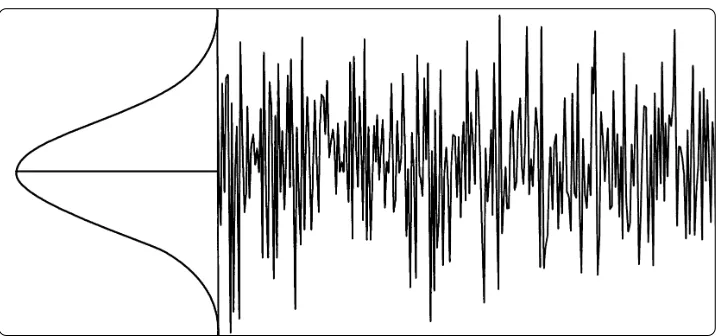
Spectrum analyzers display signals plus their own internal noise,2as shown in figure 24. To reduce
the effect of noise on the displayed signal ampli-tude, we often smooth or average the display, as shown in figure 25. All Agilent superheterodyne analyzers include a variable video filter for this purpose. The video filter is a low-pass filter that follows the detector and determines the bandwidth of the video circuits that drive the vertical deflec-tion system of the display. As the cutoff frequency of the video filter is reduced to the point at which it becomes equal to or less than the bandwidth of the selected resolution (IF) filter, the video system can no longer follow the more rapid variations of the envelope of the signal(s) passing through the IF chain. The result is an averaging or smoothing of the displayed signal.
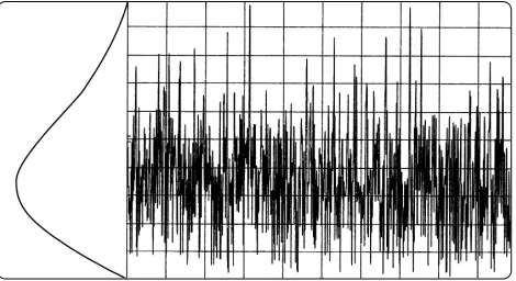
Figure 25. Display of figure 24 after full smoothing
19
The effect is most noticeable in measuring noise, particularly when a wide resolution bandwidth is used. As we reduce the video bandwidth, the peak-to-peak variations of the noise are reduced. As fig-ure 26 shows, the degree of reduction (degree of averaging or smoothing) is a function of the ratio of the video to resolution bandwidths. At ratios of 0.01 or less, the smoothing is very good; at higher ratios, not so good. That part of the trace that is already smooth - for example, a sinusoid displayed well out of the noise - is not affected by the video filter.
(If we are using an analyzer with a digital display and "pos peak" display mode1, we notice two
things: changing the resolution bandwidth does not make much difference in the peak-to-peak fluctua-tions of the noise, and changing the video band-width seems to affect the noise level. The fluctua-tions do not change much because the analyzer is displaying only the peak values of the noise. However, the noise level appears to change with video bandwidth because the averaging [smooth-ing] changes, thereby changing the peak values of the noise. See figure 27. We can select sample detection to get the full effect.)
Because the video filter has its own response time, the sweep time equation becomes: ST = k(Span)/[(RBW)(VBW)] when the video bandwidth is equal to or less than the resolution bandwidth. However, sweep time is affected only when the value of the signal varies over the span selected. For example, if we were experimenting with the analyzer’s own noise in the example above, there would be no need to slow the sweep because the average value of the noise is constant across a very wide frequency range. On the other hand, if there is a discrete signal in addition to the noise, we must slow the sweep to allow the video filter to respond to the voltage changes created as the mixing product of the discrete signal sweeps past the IF. Those analyzers that set sweep time automatically account for video bandwidth as well as span and resolution bandwidth.
Figure 26. Smoothing effect of video-resolution bandwidth ratios of 3, 1/10, and 1/100 (on a single sweep)
Figure 27. On analyzers using pos peak display mode, reducing the video bandwidth lowers the peak noise but not the average noise. Lower trace shows average noise.
20
Video averaging
Analyzers with digital displays often offer another choice for smoothing the display: video averaging. In this case, averaging is accomplished over two or more sweeps on a point-by-point basis. At each dis-play point, the new value is averaged in with the previously averaged data:
Aavg= [(n - 1)/n]Aprior avg+ (1/n)An,
where Aavg = new average value,
Aprior avg= average from prior sweep, An= measured value on current sweep, and n = number of current sweep.
Thus the display gradually converges to an average over a number of sweeps. As with video filtering, we can select the degree of averaging or smoothing by setting the number of sweeps over which the averaging occurs. Figure 28 shows video averaging for different numbers of sweeps. While video aver-aging has no effect on sweep time, the time to reach a given degree of averaging is about the same as with video filtering because of the number of sweeps required1.
Which form of display smoothing should we pick? In many cases, it does not matter. If the signal is noise or a low-level sinusoid very close to the noise, we get the same results with either video fil-tering or video averaging.
However, there is a distinct difference between the two. Video filtering performs averaging in real time; that is, we see the full effect of the averaging or smoothing at each point on the display as the sweep progresses. Each point is averaged only once, for a time of about 1/VBW on each sweep. Video averaging, on the other hand, requires multi-ple sweeps to achieve the full degree of averaging, and the averaging at each point takes place over the full time period needed to complete the multi-ple sweeps.
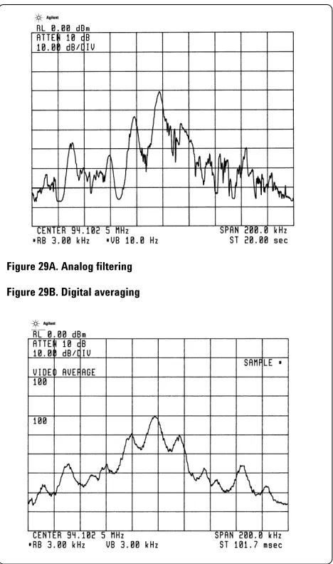
As a result, we can get significantly different results from the two averaging methods on certain signals. For example, a signal with a spectrum that changes with time can yield a different average on each sweep when we use video filtering. However, if we choose video averaging over many sweeps, we shall get a value much closer to the true average. See figure 29.
[image:20.612.312.546.248.644.2]Figure 28. Effect of video (digital) averaging for 1, 5, 20, and 100 sweeps (top to bottom)
Figure 29A. Analog filtering
Figure 29B. Digital averaging
Figure 29. Video (analog) filtering and video (digital) averaging yield different results on an FM broadcast signal
21
Amplitude measurements
CRT displays
Up until the mid-1970s, spectrum analyzer displays were purely analog. That is, the output of the enve-lope detector was simply amplified and applied directly to the vertical plates of the CRT. This mode of operation meant that the CRT trace pre-sented a continuous indication of the signal enve-lope, and no information was lost. However, analog displays had drawbacks. The major problem was in handling the long sweep times when narrow reso-lution bandwidths were used. In the extreme case, the display became a spot that moved slowly across the CRT with no real trace on the display. Even with long-persistence phosphors such as P7, a meaningful display was not possible with the longer sweep times. One solution in those days was time-lapse photography.
Another solution was the storage CRT. These tubes included mechanisms to store a trace so that it could be displayed on the screen for a reasonable length of time before it faded or became washed out. Initially, storage was binary in nature. We could choose permanent storage, or we could erase the display and start over. Hewlett-Packard (now Agilent) pioneered a variable-persistence mode in which we could adjust the fade rate of the display. When properly adjusted, the old trace would just fade out at the point where the new trace was updating the display. The idea was to provide a display that was continuous, had no flicker, and avoided confusing overwrites. The system worked quite well with the correct trade-off between trace intensity and fade rate. The difficulty was that the intensity and the fade rate had to be readjusted for each new measurement situation.
22
Digital displays
But digital systems were had problems of their own. What value should be displayed? As figure 30 shows, no matter how many data points we use across the CRT, each point must represent what has occurred over some frequency range and, although we usually do not think in terms of time when dealing with a spectrum analyzer, over some time interval. Let us imagine the situation illustrat-ed in figure 30: we have a display that contains a single CW signal and otherwise only noise. Also, we have an analog system whose output we wish to display as faithfully as possible using digital techniques.
As a first method, let us simply digitize the instan-taneous value of the signal at the end of each interval (also called a cell or bucket). This is the sample mode. To give the trace a continuous look, we design a system that draws vectors between the points. From the conditions of figure 30, it appears that we get a fairly reasonable display, as shown in figure 31. Of course, the more points in the trace, the better the replication of the analog signal. The number of points is limited, with 400, 600, 800, and 1,000 being typical.1As shown in figure 32,
more points do indeed get us closer to the analog signal.
While the sample mode does a good job of indicat-ing the randomness of noise, it is not a good mode for a spectrum analyzer's usual function: analyzing sinusoids. If we were to look at a 100-MHz comb on the Agilent 71210, we might set it to span from 0 to 22 GHz. Even with 1,000 display points, each point represents a span of 22 MHz, far wider than the maximum 3-MHz resolution bandwidth.
Figure 30. When digitizing an analog signal, what value should be displayed at each point?
Figure 31. The sample display mode using ten points to display the signal of figure 30
Figure 32. More points produce a display closer to an analog display
23
As a result, the true amplitude of a comb tooth is shown only if its mixing product happens to fall at the center of the IF when the sample is taken. Figure 33 shows a 5-GHz span with a 1-MHz band-width; the comb teeth should be relatively equal in amplitude. Figure 34 shows a 500-MHz span com-paring the true comb with the results from the sample mode; only a few points are used to exag-gerate the effect. (The sample trace appears shifted to the left because the value is plotted at the begin-ning of each interval.)
One way to insure that all sinusoids are reported is to display the maximum value encountered in each cell. This is the positive-peak display mode, or pos peak. This display mode is illustrated in figure 35. Figure 36 compares pos peak and sample play modes. Pos peak is the normal or default dis-play mode offered on many spectrum analyzers because it ensures that no sinusoid is missed, regardless of the ratio between resolution band-width and cell band-width. However, unlike sample mode, pos peak does not give a good representa-tion of random noise because it captures the crests of the noise. So spectrum analyzers using the pos peak mode as their primary display mode generally also offer the sample mode as an alternative.
To provide a better visual display of random noise than pos peak and yet avoid the missed-signal problem of the sample mode, the Rosenfell display mode is offered on many spectrum analyzers. Rosenfell is not a person’s name but rather a description of the algorithm that tests to see if the signal rose and fell within the cell represented by a given data point. Should the signal both rise and fall, as determined by pos-peak and neg-peak detectors, then the algorithm classifies the signal as noise. In that case, an odd-numbered data point indicates the maximum value encountered during its cell. On the other band, an even-numbered data point indicates the minimum value encountered during its cell. Rosenfell and sample modes are compared in figure 37.
Figure 33. A 5-GHz span of a 100-MHz comb in the sample display mode. The actual comb values are relatively constant over this range.
Figure 34. The actual comb and results of the sample display mode over a 500-MHz span. When resolution bandwidth is narrower than the sam-ple interval, the samsam-ple mode can give erroneous results. (The samsam-ple trace has only 20 points to exaggerate the effect.)
Figure 35. Pos peak display mode versus actual comb
Figure 36. Comparison of sample and pos peak display modes
24
What happens when a sinusoidal signal is encoun-tered? We know that as a mixing product is swept past the IF filter, an analyzer traces out the shape of the filter on the display. If the filter shape is spread over many display points, then we
encounter a situation in which the displayed signal only rises as the mixing product approaches the center frequency of the filter and only falls as the mixing product moves away from the filter center frequency. In either of these cases, the pos-peak and neg-peak detectors sense an amplitude change in only one direction, and, according to the
Rosenfell algorithm, the maximum value in each cell is displayed. See figure 38.
What happens when the resolution bandwidth is narrow relative to a cell? If the peak of the response occurs anywhere but at the very end of the cell, the signal will both rise and fall during the cell. If the cell happens to be an odd-numbered one, all is well. The maximum value encountered in the cell is simply plotted as the next data point. However, if the cell is even-numbered, then the minimum value in the cell is plotted. Depending on the ratio of resolution bandwidth to cell width, the minimum value can differ from the true peak value (the one we want displayed) by a little or a lot. In the extreme, when the cell is much wider than the resolution bandwidth, the difference between the maximum and minimum values encountered in the cell is the full difference between the peak signal value and the noise. Since the Rosenfell algorithm calls for the minimum value to be indicated during an even-numbered cell, the algorithm must include some provision for preserving the maximum value encountered in this cell.
To ensure no loss of signals, the pos-peak detector is reset only after the peak value has been used on the display. Otherwise, the peak value is carried over to the next cell. Thus when a signal both rises and falls in an even-numbered cell, and the mini-mum value is displayed, the pos-peak detector is not reset. The pos-peak value is carried over to the next cell, an odd-numbered cell. During this cell, the pos-peak value is updated only if the signal value exceeds the value carried over. The displayed value, then, is the larger of the held-over value and the maximum value encountered in the new, odd-numbered cell. Only then is the pos-peak detector reset.
This process may cause a maximum value to be displayed one data point too far to the right, but the offset is usually only a small percentage of the span. Figure 39 shows what might happen in such a case. A small number of data points exaggerate the effect.
Figure 38. When detected signal only rises or falls, as when mixing product sweeps past resolution filter, Rosenfell displays maximum values
Figure 39. Rosenfell when signal peak falls between data points (fewer trace points exaggerate the effect)
The Rosenfell display mode does a better job of combining noise and discrete spectral components on the display than does pos peak. We get a much better feeling for the noise with Rosenfell.
However, because it allows only maxima and mini-ma to be displayed, Rosenfell does not give us the true randomness of noise as the sample mode does. For noise signals, then, the sample display mode is the best.
Agilent analyzers that use Rosenfell as their default, or normal, display mode also allow selec-tion of the other display modes - pos peak, neg peak, and sample.
25
Amplitude accuracy
Now that we have our signal displayed on the CRT, let’s look at amplitude accuracy. Or, perhaps bet-ter, amplitude uncertainty. Most spectrum analyz-ers these days are specified in terms of both absolute and relative accuracy. However, relative performance affects both, so let us look at those factors affecting relative measurement uncertainty first.
Relative uncertainty
When we make relative measurements on an incoming signal, we use some part of the signal as a reference. For example, when we make second-harmonic distortion measurements, we use the fundamental of the signal as our reference. Absolute values do not come into play1; we are
interested only in how the second harmonic differs in amplitude from the fundamental.
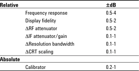
So what factors come into play? Table 1 gives us a reasonable shopping list. The range of values given covers a wide variety of spectrum analyzers. For example, frequency response, or flatness, is fre-quency-range dependent. A low-frequency RF ana-lyzer might have a frequency response of ±0.5 dB2.
[image:25.612.311.544.97.216.2]On the other hand, a microwave spectrum analyzer tuning in the 20-GHz range could well have a fre-quency response in excess of ±4 dB. Display fideli-ty covers a variefideli-ty of factors. Among them are the log amplifier (how true the logarithmic characteris-tic is), the detector (how linear), and the digitizing circuits (how linear). The CRT itself is not a factor for those analyzers using digital techniques and offering digital markers because the marker infor-mation is taken from trace memory, not the CRT. The display fidelity is better over small amplitude differences, so a typical specification for display fidelity might read 0.1 dB/dB, but no more than the value shown in table 1 for large amplitude differences.
Figure 40. Controls that affect amplitude accuracy
Table 1. Amplitude uncertainties
Relative ±dB
Frequency response 0.5-4
Display fidelity 0.5-2
6RF attenuator 0.5-2
6lF attenuator/gain 0.1-1
6Resolution bandwidth 0.1-1
6CRT scaling 0.1-1
Absolute
Calibrator 0.2-1
The remaining items in the table involve control changes made during the course of a measure-ment. See figure 40. Because an RF input attenua-tor must operate over the entire frequency range of the analyzer, its step accuracy, like frequency response, is a function of frequency. At low RF fre-quencies, we expect the attenuator to be quite good; at 20 GHz, not as good. On the other hand, the IF attenuator (or gain control) should be more accurate because it operates at only one frequency. Another parameter that we might change during the course of a measurement is resolution band-width. Different filters have different insertion losses. Generally we see the greatest difference when switching between inductor-capacitor (LC) filters, typically used for the wider resolution bandwidths, and crystal filters. Finally, we may wish to change display scaling from, say, 10 dB/div to 1 dB/div or linear.
26
A factor in measurement uncertainty not covered in the table is impedance mismatch. Analyzers do not have perfect input impedances, nor do most signal sources have ideal output impedances. However, in most cases uncertainty due to mis-match is relatively small. Improving the mis-match of either the source or analyzer reduces uncertainty. Since an analyzer’s match is worst with its input attenuator set to 0 dB, we should avoid the 0-dB setting if we can. If need be, we can attach a well-matched pad (attenuator) to the analyzer input and so effectively remove mismatch as a factor.
Absolute accuracy
The last item in table 1 is the calibrator, which gives the spectrum analyzer its absolute calibra-tion. For convenience, calibrators are typically built into today’s spectrum analyzers and provide a signal with a specified amplitude at a given fre-quency. We then rely on the relative accuracy of the analyzer to translate the absolute calibration to other frequencies and amplitudes.
Improving overall uncertainty
If we are looking at measurement uncertainty for the first time, we may well be concerned as we mentally add up the uncertainty figures. And even though we tell ourselves that these are worst-case values and that almost never are all factors at their worst and in the same direction at the same time, still we must add the figures directly if we are to certify the accuracy of a specific measurement.
There are some things that we can do to improve the situation. First of all, we should know the spec-ifications for our particular spectrum analyzer. These specifications may be good enough over the range in which we are making our measurement. If not, table 1 suggests some opportunities to
improve accuracy.
Before taking any data, we can step through a measurement to see if any controls can be left unchanged. We might find that a given RF attenua-tor setting, a given resolution bandwidth, and a given display scaling suffice for the measurement. If so, all uncertainties associated with changing these controls drop out. We may be able to trade off IF attenuation against display fidelity, using whichever is more accurate and eliminating the other as an uncertainty factor. We can even get around frequency response if we are willing to go to the trouble of characterizing our particular ana-lyzer1. The same applies to the calibrator. If we
have a more accurate calibrator, or one closer to the frequency of interest, we may wish to use that in lieu of the built-in calibrator.
Finally, many analyzers available today have self-calibration routines. These routines generate error coefficients (for example, amplitude changes ver-sus resolution bandwidth) that the analyzer uses later to correct measured data. The smaller values shown in table 1, 0.5 dB for display fidelity and 0.1 dB for changes in IF attenuation, resolution bandwidth, and display scaling, are based on cor-rected data. As a result, these self-calibration rou-tines allow us to make good amplitude measure-ments with a spectrum analyzer and give us more freedom to change controls during the course of a measurement.
27
Sensitivity
One of the primary uses of a spectrum analyzer is to search out and measure low-level signals. The ultimate limitation in these measurements is the random noise generated by the spectrum analyzer itself. This noise, generated by the random electron motion throughout the various circuit elements, is amplified by the various gain stages in the analyz-er and ultimately appears on the display as a noise signal below which we cannot make measurements. A likely starting point for noise seen on the display is the first stage of gain in the analyzer. This ampli-fier boosts the noise generated by its input termi-nation plus adds some of its own. As the noise sig-nal passes on through the system, it is typically high enough in amplitude that the noise generated in subsequent gain stages adds only a small
amount to the noise power. It is true that the input attenuator and one or more mixers may be
between the input connector of a spectrum analyz-er and the first stage of gain, and all of these com-ponents generate noise. However, the noise that they generate is at or near the absolute minimum of –174 dBm/Hz (kTB), the same as at the input termination of the first gain stage, so they do not significantly affect the noise level input to, and amplified by, the first gain stage.
While the input attenuator, mixer, and other circuit elements between the input connector and first gain stage have little effect on the actual system noise, they do have a marked effect on the ability of an analyzer to display low-level signals because they attenuate the input signal. That is, they reduce the signal-to-noise ratio and so degrade sensitivity.
We can determine sensitivity simply by noting the noise level indicated on the display with no input signal applied. This level is the analyzer’s own noise floor. Signals below this level are masked by the noise and cannot be seen or measured.
However, the displayed noise floor is not the actual noise level at the input but rather the effective noise level. An analyzer display is calibrated to reflect the level of a signal at the analyzer input, so the displayed noise floor represents a fictitious (we have called it an effective) noise floor at the input below which we cannot make measurements. The actual noise level at the input is a function of the input signal. Indeed, noise is sometimes the signal of interest. Like any discrete signal, a noise signal must be above the effective (displayed) noise floor to be measured. The effective input noise floor includes the losses (attenuation) of the input attenuator, mixer(s), etc., prior to the first gain stage.
28
Different analyzers handle the change of input attenuation in different ways. Because the input attenuator has no effect on the actual noise gener-ated in the system, some analyzers simply leave the displayed noise at the same position on the display regardless of the input-attenuator setting. That is, the IF gain remains constant. This being the case, the input attenuator will affect the loca-tion of a true input signal on the display. As we increase input attenuation, further attenuating the input signal, the location of the signal on the dis-play goes down while the noise remains stationary. To maintain absolute calibration so that the actual input signal always has the same reading, the ana-lyzer changes the indicated reference level (the value of the top line of the graticule). This design is used in older Agilent analyzers.
In newer Agilent analyzers, starting with the 8568A, an internal microprocessor changes the IF gain to offset changes in the input attenuator. Thus, true input signals remain stationary on the display as we change the input attenuator, while the displayed noise moves up and down. In this case, the reference level remains unchanged. See figures 41 and 42. In either case, we get the best signal-to-noise ratio (sensitivity) by selecting mini-mum input attenuation.
Resolution bandwidth also affects signal-to-noise ratio, or sensitivity. The noise generated in the analyzer is random and has a constant amplitude over a wide frequency range. Since the resolution, or IF, bandwidth filters come after the first gain stage, the total noise power that passes through the filters is determined by the width of the filters. This noise signal is detected and ultimately reach-es the display. The random nature of the noise sig-nal causes the displayed level to vary as:
10*log(bw2/bw1),
where bw1= starting resolution bandwidth and bw2= ending resolution bandwidth.
[image:28.612.311.545.396.556.2]Figure 41. Some spectrum analyzers change reference level when RF attenuator is changed, so an input signal moves on the display, but the analyzer’s noise does not
29
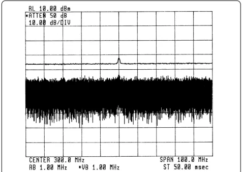
So if we change the resolution bandwidth by a fac-tor of 10, the displayed noise level changes by 10 dB1, as shown in figure 43. We get best
signal-to-noise ratio, or best sensitivity, using the minimum resolution bandwidth available in our spectrum analyzer.
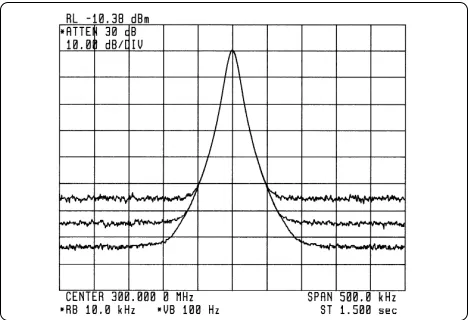
A spectrum analyzer displays signal plus noise, and a low signal-to-noise ratio makes the signal difficult to distinguish. We noted above that the video filter can be used to reduce the amplitude fluctuations of noisy signals while at the same time having no effect on constant signals. Figure 44 shows how the video filter can improve our ability to discern low-level signals. It should be noted that the video filter does not affect the average noise level and so does not, strictly speaking, affect the sensitivity of an analyzer.
In summary, we get best sensitivity by selecting the minimum resolution bandwidth and minimum input attenuation. These settings give us best sig-nal-to-noise ratio. We can also select minimum video bandwidth to help us see a signal at or close to the noise level2. Of course, selecting narrow
res-olution and video bandwidths does lengthen the sweep time.
Noise figure
Many receiver manufacturers specify the perfor-mance of their receivers in terms of noise figure rather than sensitivity. As we shall see, the two can be equated. A spectrum analyzer is a receiver, and we shall examine noise figure on the basis of a sinusoidal input.
Noise figure can be defined as the degradation of signal-to-noise ratio as a signal passes through a device, a spectrum analyzer in our case. We can express noise figure as:
F = (Si/Ni)/(So/No),
where F= noise figure as power ratio, Si = input signal power,
[image:29.612.310.545.50.224.2]Ni = true input noise power, So= output signal power, and No= output noise power.
[image:29.612.308.546.261.430.2]Figure 43. Displayed noise level changes as 10*log(BW2/BW1)
Figure 44. Video filtering makes low-level signals more discernable. (The average trace was offset for visibility.)
If we examine this expression, we can simplify it for our spectrum analyzer. First of all, the output signal is the input signal times the gain of the ana-lyzer. Second, the gain of our analyzer is unity because the signal level at the output (indicated on the display) is the same as the level at the input (input connector). So our expression, after substi-tution, cancellation, and rearrangement, becomes:
F = No/Ni
This expression tells us that all we need to do to determine the noise figure is compare the noise level as read on the display to the true (not the effective) noise level at the input connector. Noise figure is usually expressed in terms of dB, or:
NF = 10*log(F) = 10*log(No) - 10*log(Ni).
1 Not always true for the analyzer’s own noise because of the way IF step gain and filter poles are distributed throughout the IF chain. However, the relationship does hold true when the noise is the external signal being measured.
30
We use the true noise level at the input rather than the effective noise level because our input signal-to-noise ratio was based on the true noise. Now we can obtain the true noise at the input simply by terminating the input in 50 ohms. The input noise level then becomes:
Ni= kTB,
where k = Boltzmann’s constant,
T = absolute temperature in degrees Kelvin, and
B = bandwidth.
At room temperature and for a 1-Hz bandwidth,
kTB = –174 dBm.
We know that the displayed level of noise on the analyzer changes with bandwidth. So all we need to do to determine the noise figure of our spec-trum analyzer is to measure the noise power in some bandwidth, calculate the noise power that we would have measured in a 1-Hz bandwidth using 10*log(bw2/bw1), and compare that to –174 dBm. For example, if we measured –110 dBm in a 10-kHz resolution bandwidth, we would get:
NF =
(measured noise)dBm/RBW– 10*log(RBW/1) – kTBB=1
= –110 dBm – 10*log(10,000/1) – (–174 dBm) = –110 – 40 + 174
= 24 dB.
Noise figure is independent of bandwidth1. Had we selected a different resolution bandwidth, our results would have been exactly the same. For example, had we chosen a 1-kHz resolution bandwidth, the measured noise would have been –120 dBm and 10*log(RBW/1) would have been 30. Combining all terms would have given –120 – 30 + 174 = 24 dB, the same noise figure as above.
The 24-dB noise figure in our example tells us that a sinusoidal signal must be 24 dB above kTB to be equal to the average displayed noise on this partic-ular analyzer. Thus we can use noise figure to determine sensitivity for a given bandwidth or to compare sensitivities of different analyzers on the same bandwidth2.
Preamplifiers
One reason for introducing noise figure is that it helps us determine how much benefit we can derive from the use of a preamplifier. A 24-dB noise figure, while good for a spectrum analyzer, is not so good for a dedicated receiver. However, by placing an appropriate preamplifier in front of the spectrum analyzer, we can obtain a system (pream-plifier/spectrum analyzer) noise figure that is lower than that of the spectrum analyzer alone. To the extent that we lower the noise figure, we also improve the system sensitivity.
When we introduced noise figure above, we did so on the basis of a sinusoidal input signal. We shall examine the benefits of a preamplifier on the same basis. However, a preamplifier also amplifies noise, and this output noise can be higher than the effec-tive input noise of the analyzer. As we shall see in the Noise as a Signal section below, a spectrum analyzer displays a random noise signal 2.5 dB below its actual value. As we explore preamplifiers, we shall account for this 2.5-dB factor where appropriate.
1 This may not be precisely true for a given analyzer because of the way resolution filter sections and gain are distributed in the IF chain.
31
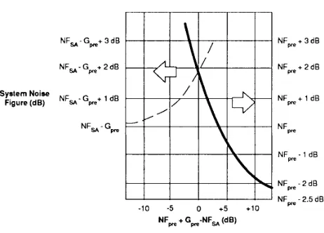
Rather than develop a lot of formulas to see what benefit we get from a preamplifier, let us look at two extreme cases and see when each might apply. First, if the noise power out of the preamplifier (in a bandwidth equal to that of the spectrum analyz-er) is at least 15 dB higher than the displayed average noise level (noise floor) of the spectrum analyzer, then the noise figure of the system is approximately that of the preamplifier less 2.5 dB. How can we tell if this is the case? Simply connect the preamplifier to the analyzer and note what happens to the noise on the CRT. If it goes up 15 dB or more, we have fulfilled this requirement.
On the other hand, if the noise power out of the preamplifier (again, in the same bandwidth as that of the spectrum analyzer) is 10 dB or more lower than the average displayed noise level on the ana-lyzer, then the noise figure of the system is that of the spectrum analyzer less the gain of the pream-plifier. Again we can test by inspection. Connect the preamplifier to the analyzer; if the displayed noise does not change, we have fulfilled the requirement.
But testing by experiment means that we have the equipment at hand. We do not need to worry about numbers. We simply connect the preamplifier to the analyzer, note the average displayed noise level and subtract the gain of the preamplifier. Then we have the sensitivity of the system.
What we really want is to know ahead of time what a preamplifier will do for us. We can state the two cases above as follows:
if NFPRE + GPRE * NFSA+ 15 dB,
then NFSYS = NFPRE– 2.5 dB,
and
if NFPRE+ GPRE ) NFSA– 10 dB,
then NFSYS = NFSA– GPRE.
Using these expressions, let’s see how a preampli-fier affects our sensitivity. Assume that our spec-trum analyzer has a noise figure of 24 dB and the preamplifier has a gain of 36 dB and a noise figure of 8 dB. All we need to do is to compare the gain plus noise figure of the preamplifier to the noise figure of the spectrum analyzer. The gain plus noise figure of the preamplifier is 44 dB, more than 15 dB higher than the noise figure of the spectrum analyzer, so the noise figure of the pre-amplifier/spectrum-analyzer combination is that of the preamplifier less 2.5 dB, or 5.5 dB. In a 10-kHz resolution bandwidth our preamplifier/analyzer system has a sensitivity of:
kTBB=1+ 10*log(RBW/1) + NFSYS
= –174 dBm + 40 dB + 5.5 dB = –128.5 dBm.
This is an improvement of 18.5 db over the –110 dBm noise floor without the preamplifier.
Is there any drawback to using this preamplifier? That depends upon our ultimate measurement objective. If we want the best sensitivity but no loss of measurement range, then this preamplifier is not the right choice. Figure 45 illustrates this point. A spectrum analyzer with a 24-dB noise fig-ure will have an average displayed noise level of –110 dBm in a 10-kHz resolution bandwidth. If the 1-dB compression point1for that analyzer is –10 dBm, the measurement range is 100 dB. When we connect the preamplifier, we must reduce the maximum input to the system by the gain of the pre-amplifier to –46 dBm. However, when we con-nect the preamplifier, the noise as displayed on the CRT will rise by about 17.5 dB because the noise power out of the preamplifier is that much higher than the analyzer’s own noise floor, even after accounting for the 2.5-dB factor. It is from this higher noise level that we now subtract the gain of the preamplifier. With the preamplifier in place, our measurement range is 82.5 dB, 17.5 dB less than without the preamplifier. The loss in mea-surement range equals the change in the displayed noise when the preamplifier is connected.
32
Figure 45. If the displayed noise goes up when a preamplifier is con-nected, measurement range is diminished by the amount the noise changes
Is there a preamplifier that will give us better sen-sitivity without costing us measurement range? Yes. But it must meet the second of the above crite-ria; that is, the sum of its gain and noise figure must be at least 10 dB less than the noise figure of the spectrum analyzer. In this case the displayed noise floor will not change noticeably when we connect the preamplifier, so although we shift the whole measurement range down by the gain of the preamplifier, we end up with the same overall range that we started with.
To choose the correct preamplifier, we must look at our measurement needs. If we want absolutely the best sensitivity and are not concerned about measurement range, we would choose a high-gain, low-noise-figure preamplifier so that our system would take on the noise figure of the preamplifier less 2.5 dB. If we want better sensitivity but cannot afford to give up any measurement range, we must choose a lower-gain preamplifier.
Interestingly enough, we can use the input attenua-tor of the spectrum analyzer to effectively degrade its the noise figure (or reduce the gain of the pre-amplifier, if you prefer). For example, if we need slightly better sensitivity but cannot afford to give up any measurement range, we can use the above preamplifier with 30 dB of RF input attenuation on the spectrum analyzer. This attenuation increases the noise figure of the analyzer from 24 to 54 dB. Now the gain plus noise figure of the preamplifier (36 + 8) is 10 dB less than the noise figure of the analyzer, and we have met the conditions of the second criterion above. The noise figure of the sys-tem is now: NFsys= NFSA – GPRE= 54 dB – 36 dB = 18 dB, a 6-dB improvement over the noise figure of
the analyzer alone with 0 dB of input attenuation. So we have improved sensitivity by 6 dB and given up virtually no measurement range.
Of course, there are preamplifiers that fall in between the extre