Munich Personal RePEc Archive
Estimating multivariate GARCH and
stochastic correlation models equation by
equation
Francq, Christian and Zakoian, Jean-Michel
2014
Online at
https://mpra.ub.uni-muenchen.de/54250/
Estimating multivariate GARCH and stochastic
corre-lation models equation by equation
Christian Francq
CREST and Université Lille 3 (EQUIPPE)
Jean-Michel Zakoïan
CREST and Université Lille 3 (EQUIPPE)
March 8, 2014
Abstract. A new approach is proposed to estimate a large class of multivariate volatility mod-els. The method is based on estimating equation-by-equation the volatility parameters of the individual returns by quasi-maximum likelihood in a first step, and estimating the correlations based on volatility-standardized returns in a second step. Instead of estimating ad-multivariate volatility model we thus estimatedunivariate GARCH-type equations plus a correlation matrix, which is generally much simpler and numerically efficient. The strong consistency and asymp-totic normality of the first-step estimator is established in a very general framework. For gen-eralized constant conditional correlation models, and also for some time-varying conditional correlation models, we obtain the asymptotic properties of the two-step estimator. Our estima-tor can also be used to test the restrictions imposed by a particular MGARCH specification. An application to financial series illustrates the interest of the approach.
Keywords: Constant conditional correlation, Dynamic conditional correlation, Markov switching models, Multivariate GARCH, Quasi maximum likelihood estimation.
Address for correspondence: Jean-Michel Zakoïan, CREST, 15 Boulevard Gabriel Péri, 92245 Malakoff cedex.
1. Introduction
Generalized Autoregressive Conditional Heteroskedasticity (GARCH) models have featured prominently in the analysis of financial time series. The versions initially stressed in the econometric literature (see Engle (1982) and Bollerslev (1986)) are univariate. The last twenty years have witnessed significant research devoted to the multivariate extension of the concepts and models developed for univariate GARCH. Among the numerous speci-fications of multivariate GARCH (MGARCH) models, the most popular seem to be the Constant Conditional Correlations (CCC) model introduced by Bollerslev (1990) and ex-tended by Jeantheau (1998), the BEKK model developed by Baba, Engle, Kraft and Kroner, in a preliminary version of Engle and Kroner (1995), and the Dynamic Conditional Corre-lations (DCC) models proposed by Tse and Tsui (2002) and Engle (2002). Reviews on the rapidly changing literature on MGARCH are Bauwens, Laurent and Rombouts (2006), Sil-vennoinen and Teräsvirta (2009), Francq and Zakoïan (2010, Chapter 11), Bauwens, Hafner and Laurent (2012).
The complexity of MGARCH models has been a major obstacle to their use in applied works. Indeed, in asset pricing applications or portfolio management, cross-sections of hundreds of stocks are common. However, as the dimension of the cross section increases, the number of parameters can become very large in MGARCH models, making estimation increasingly cumbersome. This "dimensionality curse" is general in multivariate time series, but is particularly problematic in GARCH models. The reason is that the parameters of interest are involved in the conditional variance matrix, which has to be inverted in gaussian likelihood-based estimation methods.
who introduced the Dynamic Equicorrelation (DECO) model.
A solution to the high-dimension problem which does not preclude a high-dimensional parameter set relies on estimatingequation by equation the conditional variances of each component of a vector of returns. The conditional variance of component kis a function, parameterized by some parameter vectorθ(k), of the past ofall componentsof the vector of returns. Thus, the univariate models of the components are generally not GARCH in the classical sense. This approach has been used in several empirical studies (see e.g. Sucarrat, Grønneberg and Escribano (2013) for a recent reference) but asymptotic results are lacking. We propose an Equation-by-Equation (EbE) method of estimation, based on the Quasi-Maximum Likelihood (QML), for the volatility parameters θ(k) and, under appropriate assumptions, we develop an asymptotic theory for such EbE estimators (EbEE).
Apart from the numerical simplicity, one advantage of this approach is that the deriva-tion of EbEE is independent from the specificaderiva-tion of a condideriva-tional correladeriva-tion matrix. It can therefore be employed for CCC GARCH models as well as for DCC GARCH models, leading to the same estimators of the individual volatilities. It can also be used for mul-tivariate models that are not GARCH. We consider a class ofStochastic Correlation (SC) models which has the same multiplicative form as GARCH-type models, except that the correlation matrix is not a measurable function of the past observations. The term stochas-tic correlation obviously refers to the class of Stochasstochas-tic Volatility models, which differ from GARCH by the fact that the volatility depends on unobservable stochastic factors.
Estimation of the individual conditional variances can be completed, in a second step, by the estimation of a time-varying correlation matrix using the standardized returns obtained in the first step. For CCC models, the constant conditional correlation matrix can be estimated by the empirical correlation matrix of the EbEE residuals. For some DCC and SC models, the structure of the time-varying correlation can also be estimated by modeling the dynamics of the EbEE residuals. In this article, we derive asymptotic results for this estimator, which can be seen as an extension of the two-step estimator proposed by Engle and Sheppard (2001) in the case where the individual volatilities have pure GARCH forms with iid innovations. The present paper considers augmented GARCH individual volatilities depending on lagged values of all the components of the returns, with the possibility of volatility spillovers, and also enables the estimation of more complex correlation matrices.
the class of multivariate processes studied in this article. Such assumptions are discussed under different assumptions on the correlation matrix Rt. In Section 3, we study the estimation of the volatility parameters without any assumption onRt. Section 4 develops the two-step estimation method in the case of constant conditional correlation and stochastic correlation matrices. Consistency and asymptotic normality of the estimator are established. Section 5 studies testing the adequacy of a class of multivariate models. In Section 6, we apply our method to a large set of stock market indices, and to several exchange rate series. Section 7 concludes. The most technical assumptions and the proofs of the main theorems are collected in the Appendix.
2. Models and assumptions
Letǫt = (ǫ1t,· · ·, ǫmt)′ be a Rm-valued process and let Ftǫ−1 be theσ-field generated by {ǫu, u < t}. Assume
E(ǫt| Ftǫ−1) =0, (2.1)
and
Var(ǫt| Ftǫ−1) =Ht exists and is positive definite. (2.2)
Denoting byσ2
ktthe diagonal elements ofHt, that is the variances of the components ofǫt conditional onFǫ
t−1, we introduce the vector
η∗t =D−1t ǫt= (ǫ1t/σ1t, . . . , ǫmt/σmt)′ whereDt=diag(σ1t, . . . , σmt).
By (2.1)-(2.2), we haveE(η∗t | Ftǫ−1) = 0 and the conditional correlation matrix ofǫt is given by
Rt=Var(η∗t | Ftǫ−1) =D−1t HtD−1t .
It follows that, fork= 1, . . . , m,
E(η∗kt| Ftǫ−1) = 0, Var(η∗kt| Ftǫ−1) = 1. (2.3)
Introducing the vectorηtsuch thatη∗t =R 1/2
t ηt, the previous equations can be summarized as follows. The square root has to be understood in the sense of the Cholesky factorization, that is,R1t/2(R
1/2
t )′=RtandH1t/2(H 1/2
Assumptions and notations: The Rm-valued process(ǫt) satisfies
ǫt = H1t/2ηt, E(ηt| Ftǫ−1) =0, Var(ηt| Ftǫ−1) =Im,
Ht = H(ǫt−1,ǫt−2, . . .) =DtRtDt,
(2.4)
whereDt=diag(H 1/2
t )andRt=Corr(ǫt,ǫt| Ftǫ−1).
We assume that the conditional variance of the k-th component of ǫt is parameterized by some parameterθ(0k)∈Rdk, so that
ǫkt = σktη∗kt,
σkt = σk(ǫt−1,ǫt−2, . . .;θ(0k)),
(2.5)
whereσk : R∞×Θk →(0,∞). In view of (2.3), the process(η∗t)can be called the vector ofEquation-by-Equation(EbE) innovations of(ǫt).
Remark 2.1. In this model, the volatility of any component ofǫtis allowed to depend on the past values of all components. For this reason, Model (2.5) can be referred to as an
augmented GARCHmodel. Moreover, the innovationsη∗
kt are not iid. Thus, (2.5) is not a Data Generating Process (DGP).
We now consider two classes of DGP satisfying the previous assumptions.
2.1. GARCH-type models
Consider a GARCH process, defined as a non anticipative1solution of
ǫt=DtR1t/2ηt, where(ηt)is an iid sequence. (2.6)
Obviously,(ǫt)thus satisfies (2.4). A variety of parametric forms of function H has been introduced in the literature. In the GARCH literature, it is usual to distinguish Constant Conditional Correlation (CCC) models, for which
Rt=Ris a constant correlation matrix, (2.7)
from Dynamic Conditional Correlation (DCC) models whereRtis a non constant function of the past ofǫt, that is,
Rt=R(ǫt−1,ǫt−2, . . .)6=R.
1that isǫt∈ Fη
Note that in the case of CCC models, the sequence (η∗t)is iid which is generally not the case for DCC models.
2.2. Stochastic Correlation Models
To obtain a DGP satisfying (2.4), an alternative to GARCH-type models is to introduce correlation matrices that are not function of the past but also depend on some latent process
(∆t). More precisely, let
ǫt=DtR∗1t /2ξt, (2.8)
where(ξt)is an iid(0,Im)sequence and
R∗t =R∗(ǫt−1,ǫt−2, . . . ,∆t), ∆t∈ F/ tǫ−1. (2.9)
By analogy with the so-called Stochastic Volatility models, in which the volatility is not a measurable function of the past observables, we can call model (2.8)-(2.9) a Stochastic Correlation(SC) model. For this model, the individual volatilitiesσkt, as given by (2.5), are of GARCH-type, while the correlations between components inR∗t are not. In this context, a non anticipative solution of the model is such that ǫt ∈ Ftξ,∆, the σ-field generated by {ξu,∆u, u≤t}. Assuming that
(ǫt)is a non anticipative solution andξtis independent fromFt∆, (2.10)
theσ-field generated by{∆u, u≤t}, we haveE(ǫt| Ftǫ−1) =0,and
Ht = Var(ǫt| Ftǫ−1) =DtE(R∗1t /2ξtξ′tR ∗′1/2
t | Ftǫ−1)Dt=DtE(R∗t | Ftǫ−1)Dt, using the fact that E(ξtξ′t) = Im. Note that the conditional correlation matrix is Rt = E(R∗t | Fǫ
t−1).
Therefore, SC models (2.8)-(2.10), which are extensions of GARCH-type models, satisfy Assumptions (2.4). Note that the three innovations sequences are linked by
η∗t =R∗1t /2ξt=R1t/2ηt.
3. Equation-by-equation estimation of volatility parameters
To estimateθ(0k)we will use the Gaussian QML, which is the most widely used estimation method for univariate GARCH models, but other methods could be considered as well (for instance the LAD method or the weighted QML studied by Ling (2007), the non Gaussian QML studied by Berkes and Horváth (2004)). In view of Remark 2.1, Model (2.5) is not, in general, a univariate GARCH and we cannot directly rely on existing results for its estimation.
Given observations ǫ1, . . . ,ǫn, and arbitrary initial values ˜ǫi for i ≤ 0, we define
˜
σkt(θ(k)) = σk(ǫt−1,ǫt−2, . . . ,ǫ1,˜ǫ0,˜ǫ−1, . . .;θ(k)) for k = 1, . . . , m and θ(k) ∈ Θk, as-suming thatΘk is a compact parameter set andθ(k)
0 ∈Θk. This random variable will be used as a proxy ofσkt(θ(k)) =σk(ǫt−1,ǫt−2, . . . ,ǫ1,ǫ0,ǫ−1, . . .;θ(k)).
Letθˆ(nk)denote the equation-by-equation estimator (EbEE) ofθ(0k):
ˆ
θ(nk)= arg min θ(k)∈Θ(k)
˜
Q(nk)(θ (k)
), Q˜(nk)(θ (k)
) = 1
n n
X
t=1
log ˜σ2kt
θ(k)+ ǫ
2 kt
˜
σ2 kt
θ(k) .
Similarly, define
Q(nk)(θ(k)) =
1
n n
X
t=1
logσ2kt
θ(k)+ ǫ
2 kt σ2
kt
θ(k)
:= 1
n n
X
t=1
ℓkt(θ(k)).
3.1. Consistency and asymptotic normality of the EbEE
We make the following assumption on the process(ǫt).
A1: (ǫt)is a strictly stationary and ergodic process satisfying (2.4), withE|ǫkt|s<∞for somes >0. Moreover,Elogσ2
kt<∞.
This assumption can be made more explicit for specific models (see for instance Theorem 2.1 and Corollary 2.2 in Francq and Zakoian (2012)). Technical assumptions on the function σk are relegated to Appendix A. AssumptionsA4-A6are required for the consistency. To prove the asymptotic normality, we need to assume
A7: θ(0k) belongs to the interior ofΘ(k),
A8: E|η∗ kt|
4(1+δ)
<∞, for someδ >0,
Theorem 3.1. IfA1andA4-A6hold, then
ˆ
θ(nk)→θ (k)
0 , a.s. asn→ ∞.
If, in addition,A7-A12 hold, then
√nˆ θ(nk)−θ
(k) 0
L
→ N0,J−1kkIkkJ−1kk ,
where
Ikk=E {ηkt∗4−1}dktd′kt
, Jkk=E dktd′kt
, dkt=
1
σ2 kt
∂σ2 kt(θ
(k) 0 ) ∂θ(k) .
Note that the sequence of (ηt) in (2.4) is not assumed to be iid. This sequence is only assumed to be a conditionally homoscedastic martingale difference, which allows us to encompass SC models. The analogous of this result was established, in the case of semi-strong univariate GARCH(p, q) models, by Escanciano (2009) as an extension of Berkes, Horváth and Kokoszka (2003) and Francq and Zakoïan (2004).
An important class for which Theorem 3.1 applies is the class of DCC models. To our knowledge, no asymptotic estimation results exist in the literature for such models (except the consistency in the corrected "cDCC" version of Aielli (2013)). Stationarity conditions for DCC models have been recently established by Fermanian and Malongo (2014).
3.2. Efficiency loss with respect to the full QMLE?
It can be shown that estimating the volatility coefficients equation by equation does not always entail efficiency loss with respect to the full QML. To see this we compare the efficiency of the full QML estimator (FQMLE) and the EbEE in the bivariate case where, for simplicity, the only unknown coefficients are the parameters of the first volatility. We also assume a constant (and known) correlation matrix. More precisely, consider the model
ǫt=H1t/2ηt, Ht=
σ
2 1t(θ
(1)
0 ) ρ0σ1t(θ(1)0 )σ2t ρ0σ1t(θ(1)0 )σ2t σ22t
where(ηt)is as in Model (2.6).
more efficient than the EbEE. The next result shows that this is not always the case. The FQMLE of the parameterθ(1)0 is obtained by minimizingPnt=1lt(θ(1))where
lt(θ(1)) = log(1−ρ20) + logσ12t+ logσ22t+
1 1−ρ2
0
ǫ2 1t σ2
1t
+ ǫ
2 2t σ2
2t−
2ρ0ǫ1tǫ2t σ2
1tσ22t
,
withσ1t=σ1t
θ(1). Lettingζ=Varn1− 1 1−ρ2
0(η
∗
1t−ρ0η2∗t)η1∗t
o
, it is shown in Appendix B.2 that the FQMLE is asymptotically strictly more efficient than the QMLE based on the first equation if and only if
1−ρ2
0
2−ρ2 0
2
ζ < Eη ∗4 1t −1
4 . (3.3)
It is interesting to see that the comparison of the two asymptotic variances reduces to a comparison of real numbers. Moreover, these real numbers only depend on the errors dis-tribution, not on the parameters of the volatilities. Whenρ0= 0, the asymptotic variances by the two methods are the same. In the Gaussian case, elementary calculations show that (3.3) holds true: this is not surprising as the FQML coincides with the ML in this case. However, an opposite conclusion may hold for fat tailed distributions.
Roughly speaking, if the errors of a given equation are heavy tailed, it seems preferable to estimate the corresponding volatility without taking the other equations into account.
3.3. Asymptotic results for strong univariate models
The asymptotic distribution of the EbEE can be simplified under the assumption that
η∗ktis independent fromFtǫ−1. (3.4)
Moreover,A8can be replaced by the weaker assumption
A8∗: E|η∗ kt|
4 <∞,
and the technical assumptionsA10on the volatility function can be slightly weakened (see A10∗ in Appendix A). The asymptotic distribution of the EbEE is modified as follows.
Theorem 3.2. Under(3.4) and the assumptions of Theorem 3.1, withA8replaced by
A8∗ andA10 replaced byA10∗, we have √
nθˆ(nk)−θ (k) 0
L
→ N0,(Eη∗4kt−1)J−1kk .
3.4. Estimating conditional variances in SC models
Because SC models (2.8)-(2.10) satisfy Assumptions (2.4), the volatility parameters θ(0k) can be estimated equation by equation, and Theorem 3.1 applies.
We now discuss conditions under which (3.4) holds, in which case the asymptotic co-variance matrix of the EbEE simplifies as in Theorem 3.2. The next result shows that when the correlation matrixR∗t is a function of the latent process(∆t)and when the distribution of ξt is spherical, a slightly weaker condition than (3.4) holds. Let Fη
∗
t−1 be the σ-field generated by{η∗u, u < t}.
Proposition 3.1. Assume that the distribution ofξtis spherical and that the sequences
(∆t)and(ξt)are independent. Then, the SC model(2.8)-(2.10)withR∗t =R∗(∆t)satisfies
η∗kt is independent fromFη
∗
t−1. (3.6)
Moreover,(η∗
kt)is an iid (0,1) sequence.
Remark 3.1. It is worth noting that, under the assumptions of Proposition 3.1, the process(η∗t)is neither independent nor identically distributed in general (even if its com-ponents are iid). To see this, consider for example, forλ1, λ2∈Rand fork6=ℓ,
λ1ηkt∗ +λ2ηℓt∗ d
=k(λ1e′k+λ2e′ℓ)R ∗1/2
t kξ1={λ21+λ22+ 2λ1λ2R ∗
t(k, ℓ)}1/2ξ1,
conditionally onR∗t, where ek denotes the k-th column ofIm. The variable in the right-hand side of the latter equality is in general non independent of the past values ofη∗
t, and may also not be stationary (except whenR∗t(k, ℓ)is stationary).
Sinceη∗ t =D
−1
t ǫtwithDt∈ Ftǫ−1, it is clear thatF
η∗
t−1⊂ Ftǫ−1. Therefore (3.4) entails (3.6). Conversely, the equationǫt =Dtη∗t can be viewed as a GARCH-type model with non iid innovations(η∗t). Under appropriate assumptions on the GARCH recursion defined by Dt, the model has a solution of the form ǫt = ϕ(η∗t,η∗t−1, . . .) for some measurable functionϕ. In such a case (3.4) and (3.6) are equivalent, since we have
Fǫ
t−1=F
η∗
t−1. (3.7)
Example 3.1 (Information sets). Consider the multivariate stationary ARCH(1) model, in which the diagonal elements ofHthave the form
σ2
it=ωi+ m
X
j=1
αijǫ2j,t−1, ωi>0, αij≥0, i, j= 1, . . . , m.
Letht= (σ12t, . . . , σmt2 )′ andω= (ω1, . . . , ωm)′. We have
ht=ω+A(η∗t−1)ht−1,
whereA(η∗t−1) = (αijη∗2
j,t−1)i,j.It follows that
ht= Im+ ∞
X
k=1
A(η∗t−1). . .A(η∗t−k)
!
ω. (3.8)
Under A1, the infinite sum is well-defined and is finite componentwise. Otherwise, the norm of ht would not be finite with probability 1, and this would contradict the strict stationarity ofǫt. In view of (3.8), theσ-fields of ǫandη∗coincide, in the sense of (3.7).
A straightforward consequence of Proposition 3.1 and Theorems 3.1-3.2 is the next result.
Corollary 3.1. For Model (2.8)-(2.10), we have strong consistency ofθˆ(nk) under A1 and A4-A6. Under the assumptions of Proposition 3.1 and (3.7), and the additional as-sumptionsA7,A8∗,A9,A10∗, the asymptotic normality in (3.5)holds.
4. Estimating conditional and stochastic correlation matrices
Having estimated the individual conditional variances of a vector(ǫt)satisfying (2.4) in a first step, it is generally of interest to estimate the complete conditional variance matrix
Ht, which reduces to estimating the conditional correlationRt. We first consider the case whereRtis constant, before turning to the estimation of a SC model where the stochastic correlation matrixR∗t is driven by a Markov chain.
4.1. Estimating generalized CCC models
Let
ρ= (R21, . . . , Rm1, R32, . . . , Rm2, . . . , Rm,m−1)′=vech0(R),
denoting by vech0 the operator which stacks the sub-diagonal elements (excluding the di-agonal) of a matrix. The global parameter, denoted
ϑ= (θ(1)′, . . . ,θ(m)′,ρ′)′ := (θ′,ρ′)′ ∈Rd×[−1,1]m(m−1)/2, d=
m
X
k=1 dk,
belongs to the compact parameter setΘ= m
Y
k=1
Θk×[−1,1])m(m−1)/2.The true parameter value is
ϑ0= (θ(1)0 ′, . . . ,θ(0m)′,ρ′0)′:= (θ′0,ρ′0)′.
We now consider a two-step method for estimatingϑ0which can be summarized as follows:
(a) Estimation ofθ(0k), equation-by-equation, in the individual GARCH-type models (2.5) and extraction of the residuals of thek-th equation, ηˆ∗
kt= ˜σ −1 kt (ˆθ
(k)
)ǫkt;
(b) Computation of the empirical correlation matrix
ˆ
Rn = 1 n
n
X
t=1
ˆ
η∗t(ˆη∗t)′,
whereηˆ∗t is the vector of residuals of themequations.
Let
ˆ
ϑn=
ˆ
θ′n := (ˆθ (1)′
n , . . . ,θˆ (m)′
n ),ρˆ′n
′
, ρˆn=vech0( ˆRn).
Theorem 4.1. For the GCCC model(2.6)-(2.7), ifA1-A6hold, then
ˆ
ϑn →ϑ0, a.s. asn→ ∞.
For the asymptotic normality, we introduce the following notations. Let thed×dmatrix J∗ = ((κ∗
kℓ−1)Jkℓ) where κ∗kℓ =E ηkt∗2ηℓt∗2
, for k, ℓ = 1, . . . , m, and Jkℓ =E dktd′ℓt
. Let, forJ0=diag(J11, . . . ,Jmm)in bloc-matrix notation,
Σθ=J−1
0 J∗J−10 = (κ∗kℓ−1)J−1kkJkℓJ−1ℓℓ
.
Let also dt = (d′1t, . . . ,d′mt)′ ∈ Rd, Ωk = Edkt and Ω = (Ω′1, . . . ,Ω′m)′ ∈ Rd. Let Γ = var vech0η∗t(η∗t)
′
.Forx∈Rm, let thed×dmatricesF(x) =diag{(1−x2
x2
m)jm}, where jk= (1, . . . ,1)∈Rdk, andAkℓ=E{ηkt∗ηℓt∗F(η∗t)}. Let, fork, ℓ= 2, . . . , m, thed×dmatrixMk,ℓ−1=diagM(1)
k,ℓ−1, . . . ,M (m) k,ℓ−1
where
M(i) k,ℓ−1=
0d
i×di ifi6=k and i6=ℓ
Rk,ℓ−1Idi otherwise.
Let the d ×dm(m − 1)/2 matrices A = (A21. . .Am1 A32. . .Am,m−1) and M =
(M21. . .Mm1M32. . .Mm,m−1). Let thed×m(m−1)/2 matrices
L=A(Im(m−1)/2⊗Ω), Λ=M(Im(m−1)/2⊗Ω).
Let
Σθρ=−1
2ΣθΛ−J
−1
0 L, Σρ= 1 4Λ
′Σ
θΛ+
1
2 Λ
′
J−10 L+L′J−10 Λ
+Γ.
We need an additional assumption.
A13: Themcomponents ofηtare mutually independent random variables.
Theorem 4.2. For the GCCC model (2.6)-(2.7), if A1-A13 hold, for k = 1, . . . , m, andρ0∈(−1,1)m(m−1)/2, then
√nθˆ n−θ0
√n(ˆ ρn−ρ0)
→ NL
0,Σ:=
Σθ Σθρ
Σ′
θρ Σρ
,
andΣis a non-singular matrix.
Remark 4.1. Even though the components of θ0are estimated equation by equation, the components ofθˆn are not asymptotically independent in general. More precisely, it can be seen that
Σθ is diagonal if Cov(ηkt∗2, η∗2ℓt) = 0 for anyk6=ℓ.
Remark 4.2. In the asymptotic variance Σρ of ρˆn, the first two matrices in the sum reflect the effect of the estimation ofθ0, while the remaining matrix,Γ, is independent ofθ0. A limit case is when the components ofη∗t are serially independent, that is whenη∗t =ηt andR is the identity matrix. Then, straightforward computation shows that L=Λ=0 and thus
Σ=
Σθ 0
0 Im(m−1)/2
and Σθ=diag((κ∗11−1)J−111, . . . ,(κ∗mm−1)J−1mm)
Remark 4.3. It can be seen from the proof that AssumptionA13is only used to show thatΣis non singular.
Remark 4.4. It is worthnoting that all the matrices involved in the asymptotic covari-ance matrixΣ take the form of expectations. A simple estimator ofΣis thus obtained by replacing those expectations by their sample counterparts. For instance, it can be shown that a consistent estimator ofAkℓ is
ˆ
Akℓ=
1
n n
X
t=1
ˆ
η∗
ktηˆℓt∗F(ˆη∗t).
4.2. Estimating stochastic correlations driven by an hidden Markov chain
A natural extension of the generalized CCC model is obtained by allowing the matrixR∗t to be driven by a Markov chain. This extension was studied by Pelletier (2006). Assume that(ǫt)is generated by Model (2.8) with
R∗t =R∗(∆t), where(∆t)is a Markov chain onE ={1, . . . , N}. (4.2)
Note that the Markov chain is not observed but the number of states, N, is assumed to be known. Denoting byp(i, j) =P(∆t=j |∆t−1 =i)the transition probabilities of the Markov chain, the parameter vector is now denoted
ζ = (θ(1)′, . . . ,θ(m)′,ρ′(1), . . . ,ρ′(N),p′)′
:= (θ′,ρ′,p′)′∈Rd×[−1,1]N m(m−1)/2×[0,1]N(N−1),
where p = (p(1,2), p(1,3), . . . , p(1, N), p(2,2), . . . , p(N, N))′ and ρ(i) = vech0
{R(i)} for i= 1, . . . , N.
A common approach to estimating Hidden Markov Models (HMM) is maximum likeli-hood estimation (MLE). There is a vast literature on the estimation of HMM. To mention just a few, see for instance Baum (1972), Baum and Petrie (1966), Francq and Roussignol (1995), Francq, Roussignol and Zakoïan (2001) and the overviews by Cappé, Ryden and Moulines (2005), and Frühwirth-Schnatter (2005). In this paper, we do not use the full maximum likelihood method which is generally intractable, in particular when the regimes are not Markovian (that is, when the conditional variancesσ2
kt do not depend on a finite number of past values of ǫt). Instead, we follow a two-step approach: having estimated
estimate the remaining parameters in a second step. To this aim, we need to specify the errors distribution. We assume that
A14: the sequences(∆t)and(ξt)are mutually independent.
A15: the Markov chain(∆t)is stationary, irreducible and aperiodic.
A16: ξtis normally distributed with mean0and covariance matrixIm.
We start by considering the case where the GARCH part is absent in the dynamics (i.e.
Dt=Im in (2.8)). Letη∗1, . . . ,η∗n be observations of the HMM model
η∗t ={R∗(∆t)}1/2ξt, (4.3)
with unknown parameterϑ0= (ρ′0,p′0)′. The likelihood of the model is obtained by sum-ming, over all possible paths of the Markov chain, the probability densities at the points
(η∗
1, . . . ,η∗n):
Ln(ϑ) =
X
{e1,...,en}∈En
π(e1) ( n
Y
t=2
p(et−1, et)
) (n Y
t=1 fη∗
t(et)
)
whereπ(1), . . . , π(N)denote the stationary probabilities of the chain and, denoting by|A| the determinant of a square matrixA, forx∈Rm,
fx(i) = 1 (2π)m/2|R
∗(i)
|−1/2exp
−12x′R∗(i)−1x
.
Direct computation of the likelihood based on this formula rapidly becomes intractable as the sample size,n, increases. However, the likelihood can be expressed as a sum of products of matrices, using the following notations. For any functionf : E →R, let the matrix
P(f) =
p(1,1)f(1) · · · p(N,1)f(1)
..
. ...
p(1, d)f(N) · · · p(N, N)f(N)
, and the vectorΠ(f) =
π(1)f(1)
.. . π(N)f(N)
.
Then, following Francq and Roussignol (1997), the likelihood can be written as
Ln(ϑ) =e′ n
Y
t=2 P(fη∗
t)Π(fη∗1), (4.4)
The parameter space Θ∗ for ϑ is defined as a compact subset Θ∗
ρ × Θ∗p of [−1,1]N m(m−1)/2
×[0,1]N(N−1) which contains the true value ϑ0 and is compatible with Assumption A15 (that is, the Markov chain is stationary, irreducible and aperiodic for any parameter value p). It is also necessary to constrain the parameter space so that the parameter be identifiable. Yakowitz and Spragins (1968) showed that finite mixtures of m-dimensional Gaussian distributions (with distinct pairs(µi,Σi)of mean and covariance matrix) are identifiable. In Model (4.3), the multivariate Gaussian distributions correspond-ing to the different regimes of the Markov chain are centered. A way to ensure that the variances be different and cannot be permuted is to use the lexicographical order. Therefore, we assume that for anyρ∈Θ∗
ρ,
ρ(1)≺ρ(2)≺ · · · ≺ρ(N),
in the sense of the lexicographical order2. Let(ˆϑn)be a sequence such that
Ln(ˆϑn) = sup
ϑ∈Θ∗
Ln(ϑ). (4.5)
Theorem 4.3. For the Hidden Markov DCC model(4.3), ifA14, A15, A16hold, then
ˆ
ϑn →ϑ0, a.s. asn→ ∞.
It is possible to obtain the MLEϑˆn from (4.5), by numerical optimization of the likeli-hood computed from (4.4). It is however numerically more efficient to use the filter proposed by Hamilton (1989) for computing and optimizing the log-likelihood of an HMM model. The log-likelihood of the model (4.3) is given by
logLn(ϑ) = n
X
t=1
log1′πt|t−1⊙φ(η∗ t) ,
where all the elements of the vector 1 are equal to 1, ⊙denotes Hadamard’s product of matrices,φ(η∗t) = fη∗
t(1), . . . , fη∗t(N)
′ , and
πt|s = (P(∆t= 1|η∗s, . . . ,η∗1), . . . , P(∆t=d|η∗s, . . . ,η∗1)) ′
.
to our framework, the maximum likelihood can be obtained by starting with initial values forπ0 andϑ, and iterating until convergence the following steps:
(a) Set π1|0=π0 and
πt|t=
πt|t−1⊙φ(η∗t) 1′π
t|t−1⊙φ(η∗t)
, πt+1|t=P′πt|t, fort= 1, . . . , n.
(b) Compute the smoothed probabilitiesπt|n(i) =P(∆t=i|η∗1, . . . ,η∗n)by
πt−1|n(i) = d
X
j=1
p(i, j)πt−1|t−1(i)πt|n(j) πt|t−1(j)
fort=n, n−1, . . . ,2,
andπt−1,t|n(i, j) =P(∆t−1=i,∆t=j|η∗1, . . . ,η∗n)by
πt−1,t|n(i, j) =
p(i, j)πt−1|t−1(i)πt|n(j) πt|t−1(j)
.
(c) Replace the previous values of the parameters byπ0=π1|n,
p(i, j) = Pn
t=2πt−1,t|n(i, j)
Pn
t=2πt−1|n(i)
and, denoting by R the space of the m×m symmetric positive definite matrices, compute
R∗(i) =arg min
R∈R
log|R|+TrR−1Σ(i) (4.6)
where
Σ(i) =Pn 1 t=1πt|n(i)
n
X
t=1
η∗t(η∗t)′πt|n(i). (4.7)
In the standard version of Hamilton’s EM algorithm, the unknown coefficients are the variance matricesΣ(i)of the Gaussian distributions, and the M step consists in maximizing
N
X
i=1 n
X
t=1
logfη∗
t(i)πt|n(i) =
−1 2
N
X
i=1 n
X
t=1
log|Σ(i)|+ (η∗t)′Σ(i)−1η∗t πt|n(i)
with respect to theΣ(i)’s. The solution of this optimization problem is given explicitly by (4.7). The matrixR∗(i)defined in (4.6) can thus be interpreted as the correlation matrix which is the closest to the covariance matrix provided by the EM algorithm.
In practice, when a GARCH part is present (i.e. Dt6=Imin (2.8)), the innovationsη∗t’s are not available. Note however that, under the assumptions of Theorem 3.1, the equation-by-equation GARCH estimatorθˆn→θ0a.s. The EM algorithm can then be applied to the residualsηˆ∗t = ˜η∗t(ˆθn) = ˜D
−1
4.3. Time complexity comparison of the EbEE and the full QMLE
Bollerslev (1990) introduced the CCC-GARCH(p, q)model
ht=ω+ q
X
i=1
Aiǫt−i+ p
X
j=1
Bjht−j
whereht= σ12t,· · ·, σmt2
′
, ǫt= ǫ21t,· · · , ǫ2mt
′
, Ai and Bj are diagonalm×m matrices with positive coefficients andω= (ω1,· · ·, ωm)′ is a vector of strictly positive coefficients. An extended version of this model, called the ExtendedCCC model by He and Teräsvirta (2004), relaxes the assumption that the matricesAi andBj are diagonal. Let us compare the computation time of the EbEE with that of the FQMLE in the case of an extended CCC-GARCH(1,1)model of dimensionm, in whichA1= (αij)andB1=diag(β1, . . . , βm). The conditional variance of thek-th component of this model is thus equal to
σkt2 =ωk+ m
X
j=1
αkjǫ2j,t−1+βkσ2k,t−1.
The EbEE of all the parameters of the model requiresmestimations of univariate GARCH-type models with m+ 2 parameters, plus the computation of the empirical correlation of the EbE residuals. The full QMLE requires the optimization of a function of the m2+ 2m+m(m
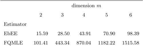
−1)/2 parameters of the model. Because the time complexity of an optimization generally grows rapidly with the dimension of the objective function, the full QMLE should be much more costly than the EbEE in terms of computation time. Ta-ble 1 compares the effective computation times required by the two estimators as a function of the dimension m, for the exchange rate series that will be studied in Section 6 below. These time series have length n = 2081. As expected, the comparison is clearly in fa-vor of the EbEE. Note that these computation times have been obtained using a single processor. Since the EbEE is clearly easily parallelizable (using one processor for each of themoptimizations), the advantage of the EbEE should be even more pronounced with a multiprocessing implementation.
5. Testing for adequacy of particular MGARCH models
Table 1. Computation time of the two estimators (CPU time in seconds)
dimensionm
2 3 4 5 6
Estimator
EbEE 15.59 28.50 43.91 70.90 98.39
FQMLE 101.41 443.34 870.04 1182.22 1515.58
strong restrictions on the volatility of the individual components. Let us focus on the class of BEKK models.
For simplicity, consider the simplest model of this form, namely the bivariate BEKK-GARCH(1,1) model given by
ǫt = H1t/2ηt, Ht=Ω+Aǫt−1ǫ′t−1A′+BHt−1, (5.1)
where (ηt) is an iidR2-valued centered sequence with Eηtη′t=I2, A= (aij)1≤i,j≤2 and B=diag(b1, b2)with b1, b2≥0, andΩ is a positive definite 2×2 matrix. It follows that the diagonal entries ofHtare given by
h11,t = ω11+a211ǫ21,t−1+ 2a11a12ǫ1,t−1ǫ2,t−1+a212ǫ22,t−1+b1h11,t−1, h22,t = ω22+a221ǫ21,t−1+ 2a21a22ǫ1,t−1ǫ2,t−1+a222ǫ22,t−1+b2h22,t−1.
Lettingθ(0k)= (ωkk, a2k1,2ak1ak2, a2k2)′fork= 1,2, the validity of this model can be studied by estimating Model (2.5) for each component ofǫt, with
σkt2 =θ (k) 01 +θ
(k)
02ǫ21,t−1+θ (k)
03ǫ1,t−1ǫ2,t−1+θ04(k)ǫ22,t−1+θ (k)
05σ2k,t−1, k= 1,2, (5.2)
under the positivity constraintsθ01(k) >0, θ0(ik) ≥ 0, i = 2,5. The restrictions implied by the BEEK-GARCH(1,1) model (5.1) are of the form:
H0(k): θ (k) 03 = 2
q
θ02(k)θ (k)
04, k= 1,2.
Let
Θ(k)=Θ∗k∩
θ(k);θ(3k)∈
0,2
q
θ2(k)θ(4k)
,
whereΘ∗k is a compact subset of {θ(k) 1 >0, θ
(k)
i ≥0,fori= 2,3,4and θ (k)
Theorem 5.1. Let the spectral radius of A+B be less than 1, and let a11a12 > 0,
a21a22 >0. Letη1 admit, with respect to the Lebesgue measure on R2, a positive density
around 0, and suppose thatE|ηkt|4(1+δ)<∞, for k= 1,2 and someδ >0. Letθ(0k) belong
to the interior ofΘ∗k for k= 1,2.
Let (ǫt) be the strictly stationary solution of Model(5.1). Let the Wald statistic for the hypothesis H0(k),
W(nk)=
n
ˆ
θ(nk3)−2
q ˆ
θ(nk2)θˆ (k) n4
2
X′nJˆ −1 kkIˆkkJˆ
−1 kkXn
, where θˆ(nk)= (ˆθn(k1), . . . ,θˆ (k) n5)′,
Xn=
0,
q ˆ
θn(k4)/θˆ (k) n2,−1,
q ˆ
θn(k2)/θˆ (k) n4,0
′ ,ηˆ∗
kt=ǫkt/σ˜kt(ˆθ (k) n )and
ˆ
Jkk= 1 n
n
X
t=1
ˆ
dktˆd ′
kt, Iˆkk= 1 n
n
X
t=1
{ηˆ∗4kt−1}dˆktdˆ ′
kt, dˆkt= 1
˜
σ2 kt(ˆθn)
∂σ˜2 kt(ˆθ
(k) n ) ∂θ(k) .
Then,W(nk) asymptotically follows a mixture of theχ2 distribution with one degree of
free-dom and the Dirac measure at 0:
W(nk) L
→ 12χ2(1) +1
2δ0 asn→ ∞.
In view of this result, testingH0(k)at the asymptotic levelα∈(0,1/2)can thus be achieved by using the critical region{W(nk)> χ21−2α(1)}.
6. Illustrations
We present two applications. The first one shows that the two-step EbEE can easily estimate a CCC-GARCH model, even if the different components of the multivariate series of returns are not observed simultaneously. In that case, the individual volatilities have however to follow pure GARCH models. In the second application, the individual volatilities are augmented GARCH models and the conditional correlation displays several regimes. The second application also illustrates the specification test based on the EbEE.
6.1. An application to world stock market indices
the daily data available over the period from 1990-01-01 to 2013-04-22, and we eliminated a few series with too few observations. We then obtained a total number of 25 series: 5 for Americas, 11 for Asia-Pacific, 8 for Europe and 1 for Middle East. Because some series do not cover the entire period and the working days are not the same for all the financial markets, the numbernof observations varies a lot, fromn= 2157for the series "NZ50" to n= 6040for "AEX.AS". We corrected the "MERV" series for the stock spilt that occurred in Brazil on 1997-03-11, and we started at 1990-08-02 for the series "GD.AT" because of the presence of unexpected variations before this date. On each of the 25 series, we fitted PGARCH(1,1) models of the form
ǫt=σtηt σδ
t =ω+α+(ǫ+t−1)δ+α−(−ǫ−t−1)δ+βσtδ−1
(6.1)
where x+ = max(x,0), x− = min(x,0), α+
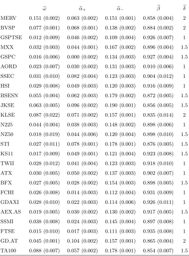
≥0, α− ≥ 0, β ∈ [0,1), ω > 0, and δ > 0. As shown by Hamadeh and Zakoian (2011), the effective estimation of the parameterδis an issue. The quasi-likelihood in the direction of δ being often relatively flat, the QML estimation of this parameter is imprecise and considerably slows down the optimization procedure. For this reason we decided to perform the QML optimization on only 4 values of this parameter: δ∈ {0.5,1,1.5,2}. For each of the 4 values ofδ, the remainder parameter θ = (ω, α+, α−, β)′ is estimated by QML. Following the (quasi-)likelihood principle, the selected values of δ and the final estimated value of θ maximize the QML over the 4 optimizations.
Table 2 displays the estimated PGARCH(1,1) models for each series, the estimated standard deviation into parentheses, and the selected value ofδin the last column. For all series, one can see a strong leverage effect (α− > α+) which means that negative returns tend to have an higher impact on the future volatility than positive returns of the same magnitude.
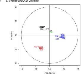
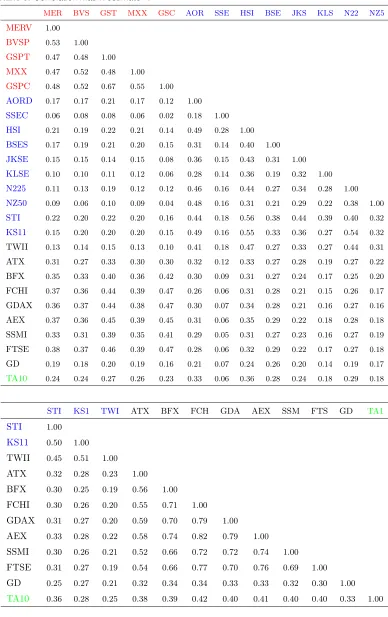
Table 3 gives an empirical estimateRˆ of the correlation matrixRof the residuals of the 25 PGARCH(1,1) equations. Because there are numerous missing values, due to the fact that the series are not always observed at the same dates, we used theRfunctioncor()with the option "use=pairwise.complete.obs", which means that the correlation between each pair of variables is computed using all complete pairs of observations on those variables.
−1.0 −0.5 0.0 0.5 1.0
−1.0
−0.5
0.0
0.5
1.0
PC2 (12.2%)
PC3 (6.5%)
MER BVS GSPT MXX GSPC
AOR
SSE HSI BSE JKSKLS
N22 NZ5
STIKS1TWI ATX
BFX FCHGDAAEXSSM
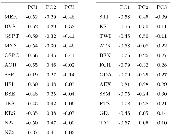
[image:23.595.122.396.111.362.2]FTS GD.TA1
Figure 1.Factorial plan PC2-PC3.
34.6%, 12.2%, 6.5% and 3.8%. Table 4 gives the so-called loading matrix, that is the correlation between the variables and the factors. From this table, it is clear that the first principal component PC1 is a scaling factor. PC1 is negatively correlated with all the series of returns. Noting that, in (6.1), the signs ofǫt andηt are the same, the PC1 factor thus opposes the days where the markets are globally profitable to days where the markets go down. Therefore, we can interpret PC1 as the global trend of the World markets (with the negative sign for PC1 when the returns are globally positive). The second factor PC2 opposes the American and European to the Asian markets, whereas PC3 opposes the European and American markets (see Figure 1 for a graphical illustration). These relationships are certainly related to the opening hours of the different markets.
6.2. An application to exchange rates
Table 2.PGARCH(1,1) models fitted by EbEE on daily returns of the major World stock indices. The estimated standard deviation are displayed into parentheses. The last column gives the selected value of the powerδ.
b
ω αb+ αb− βb bδ
MERV 0.151 (0.002) 0.063 (0.002) 0.151 (0.001) 0.858 (0.004) 2
BVSP 0.077 (0.001) 0.068 (0.001) 0.138 (0.002) 0.884 (0.002) 2
GSPTSE 0.012 (0.009) 0.046 (0.002) 0.109 (0.004) 0.926 (0.007) 1
MXX 0.032 (0.003) 0.044 (0.001) 0.167 (0.002) 0.896 (0.004) 1.5
GSPC 0.016 (0.006) 0.000 (0.002) 0.134 (0.003) 0.927 (0.004) 1.5
AORD 0.023 (0.007) 0.030 (0.002) 0.131 (0.003) 0.910 (0.006) 1
SSEC 0.031 (0.010) 0.082 (0.004) 0.123 (0.003) 0.904 (0.012) 1
HSI 0.029 (0.008) 0.049 (0.003) 0.120 (0.003) 0.916 (0.009) 1
BSESN 0.055 (0.004) 0.062 (0.003) 0.179 (0.002) 0.872 (0.005) 1.5
JKSE 0.063 (0.005) 0.096 (0.002) 0.190 (0.001) 0.856 (0.005) 1.5
KLSE 0.087 (0.022) 0.071 (0.002) 0.157 (0.001) 0.835 (0.014) 2
N225 0.044 (0.004) 0.038 (0.003) 0.148 (0.002) 0.898 (0.006) 1
NZ50 0.018 (0.019) 0.044 (0.006) 0.120 (0.004) 0.898 (0.010) 1.5
STI 0.027 (0.011) 0.078 (0.001) 0.178 (0.001) 0.876 (0.005) 1.5
KS11 0.017 (0.009) 0.049 (0.001) 0.121 (0.004) 0.923 (0.008) 1.5
TWII 0.028 (0.012) 0.041 (0.004) 0.123 (0.003) 0.918 (0.010) 1
ATX 0.030 (0.005) 0.050 (0.002) 0.137 (0.003) 0.902 (0.007) 1
BFX 0.027 (0.005) 0.028 (0.002) 0.154 (0.003) 0.898 (0.005) 1.5
FCHI 0.026 (0.008) 0.014 (0.003) 0.112 (0.004) 0.931 (0.009) 1
GDAXI 0.028 (0.010) 0.022 (0.003) 0.114 (0.006) 0.926 (0.011) 1
AEX.AS 0.019 (0.005) 0.030 (0.002) 0.130 (0.002) 0.917 (0.005) 1.5
SSMI 0.038 (0.008) 0.024 (0.003) 0.145 (0.004) 0.897 (0.008) 1
FTSE 0.015 (0.010) 0.017 (0.003) 0.111 (0.003) 0.935 (0.008) 1
GD.AT 0.045 (0.001) 0.104 (0.002) 0.157 (0.001) 0.865 (0.004) 2
Table 3.Correlation matrix estimateRˆ
MER BVS GST MXX GSC AOR SSE HSI BSE JKS KLS N22 NZ5
MERV 1.00
BVSP 0.53 1.00
GSPT 0.47 0.48 1.00
MXX 0.47 0.52 0.48 1.00
GSPC 0.48 0.52 0.67 0.55 1.00
AORD 0.17 0.17 0.21 0.17 0.12 1.00
SSEC 0.06 0.08 0.08 0.06 0.02 0.18 1.00
HSI 0.21 0.19 0.22 0.21 0.14 0.49 0.28 1.00
BSES 0.17 0.19 0.21 0.20 0.15 0.31 0.14 0.40 1.00
JKSE 0.15 0.15 0.14 0.15 0.08 0.36 0.15 0.43 0.31 1.00 KLSE 0.10 0.10 0.11 0.12 0.06 0.28 0.14 0.36 0.19 0.32 1.00
N225 0.11 0.13 0.19 0.12 0.12 0.46 0.16 0.44 0.27 0.34 0.28 1.00
NZ50 0.09 0.06 0.10 0.09 0.04 0.48 0.16 0.31 0.21 0.29 0.22 0.38 1.00
STI 0.22 0.20 0.22 0.20 0.16 0.44 0.18 0.56 0.38 0.44 0.39 0.40 0.32
KS11 0.15 0.20 0.20 0.20 0.15 0.49 0.16 0.55 0.33 0.36 0.27 0.54 0.32
TWII 0.13 0.14 0.15 0.13 0.10 0.41 0.18 0.47 0.27 0.33 0.27 0.44 0.31
ATX 0.31 0.27 0.33 0.30 0.30 0.32 0.12 0.33 0.27 0.28 0.19 0.27 0.22
BFX 0.35 0.33 0.40 0.36 0.42 0.30 0.09 0.31 0.27 0.24 0.17 0.25 0.20
FCHI 0.37 0.36 0.44 0.39 0.47 0.26 0.06 0.31 0.28 0.21 0.15 0.26 0.17
GDAX 0.36 0.37 0.44 0.38 0.47 0.30 0.07 0.34 0.28 0.21 0.16 0.27 0.16
AEX 0.37 0.36 0.45 0.39 0.45 0.31 0.06 0.35 0.29 0.22 0.18 0.28 0.18
SSMI 0.33 0.31 0.39 0.35 0.41 0.29 0.05 0.31 0.27 0.23 0.16 0.27 0.19
FTSE 0.38 0.37 0.46 0.39 0.47 0.28 0.06 0.32 0.29 0.22 0.17 0.27 0.18 GD 0.19 0.18 0.20 0.19 0.16 0.21 0.07 0.24 0.26 0.20 0.14 0.19 0.17
TA10 0.24 0.24 0.27 0.26 0.23 0.33 0.06 0.36 0.28 0.24 0.18 0.29 0.18
STI KS1 TWI ATX BFX FCH GDA AEX SSM FTS GD TA1
STI 1.00
KS11 0.50 1.00
TWII 0.45 0.51 1.00
ATX 0.32 0.28 0.23 1.00
BFX 0.30 0.25 0.19 0.56 1.00
FCHI 0.30 0.26 0.20 0.55 0.71 1.00
GDAX 0.31 0.27 0.20 0.59 0.70 0.79 1.00
AEX 0.33 0.28 0.22 0.58 0.74 0.82 0.79 1.00
SSMI 0.30 0.26 0.21 0.52 0.66 0.72 0.72 0.74 1.00
FTSE 0.31 0.27 0.19 0.54 0.66 0.77 0.70 0.76 0.69 1.00
GD 0.25 0.27 0.21 0.32 0.34 0.34 0.33 0.33 0.32 0.30 1.00
Table 4. Correlations between the variables and the first 3 factors of the PCA
PC1 PC2 PC3 PC1 PC2 PC3
MER -0.52 -0.29 -0.46 STI -0.58 0.45 -0.09
BVS -0.52 -0.29 -0.52 KS1 -0.55 0.50 -0.11
GSPT -0.59 -0.32 -0.41 TWI -0.46 0.50 -0.11
MXX -0.54 -0.30 -0.46 ATX -0.68 -0.08 0.22
GSPC -0.56 -0.45 -0.41 BFX -0.75 -0.25 0.27
AOR -0.55 0.46 -0.02 FCH -0.79 -0.32 0.28
SSE -0.19 0.27 -0.14 GDA -0.79 -0.29 0.27
HSI -0.60 0.48 -0.07 AEX -0.81 -0.28 0.29
BSE -0.48 0.25 -0.04 SSM -0.75 -0.24 0.30
JKS -0.45 0.42 -0.06 FTS -0.78 -0.28 0.21
KLS -0.35 0.38 -0.07 GD. -0.46 0.05 0.14
N22 -0.50 0.47 -0.00 TA1 -0.57 0.06 0.10
NZ5 -0.37 0.44 0.03
and cover the period from January 14, 2000 to May 16, 2013, which corresponds to 2081 observations. On these 6 series, we fitted an extended CCC-GARCH(1,1) model of the form
ht=ω+Aǫt−1+Bht−1
where Bis diagonal. This assumption allows to fit the model equation by equation. The estimated values ofAandB are
ˆ A=
0.029 0.002 0.015 0.012 0.003 0.000
0.010 0.003 0.040 0.013 0.003 0.038
0.000 0.136 0.000 0.003 0.000 0.000
0.002 0.023 0.004 0.003 0.001 0.003
0.000 0.002 0.031 0.008 0.002 0.001
0.005 0.002 0.028 0.007 0.002 0.027
0.006 0.001 0.004 0.041 0.006 0.000
0.004 0.002 0.020 0.012 0.002 0.019
0.017 0.003 0.000 0.002 0.061 0.000
0.012 0.005 0.054 0.016 0.012 0.052
0.000 0.003 0.024 0.007 0.002 0.008
0.005 0.002 0.028 0.007 0.002 0.028
, Bˆ =diag
0.92
0.022
0.88
0.017
0.95
0.010
0.93
0.015
0.93
0.014
0.96
and the estimation of the correlation matrixRis ˆ R=
1.00 0.00 0.46 0.39 0.17 0.47
0.026 0.039 0.031 0.034 0.032
0.00 1.00 0.14 0.12 0.42 0.13
0.040 0.027 0.043 0.045
0.46 0.14 1.00 0.44 0.58 0.98
0.033 0.039 0.031
0.39 0.12 0.44 1.00 0.26 0.45
0.071 0.040
0.17 0.42 0.58 0.26 1.00 0.57
0.044
0.47 0.13 0.98 0.45 0.57 1.00 CAD CHF CNY GBP JPY USD
The estimated standard deviations of the estimators were obtained from Theorem 4.2 and are displayed in small font size. It can be noted that the volatilities of the different exchange rates are mainly linked by the strong correlations of the residuals, which can be interpreted as a sign of instantaneous causality between the squared returns. By contrast, in view of the diagonal form of Aˆ, the volatility of a given exchange rate is mainly explained by its own past returns. A noticeable exception is the volatility of the USD which shows more sensitivity to the variations of the CNY than to its own variations. These two exchange rates are also strongly related by the correlation (0.98) between their rescaled residuals.
We now relax the constant correlation assumption (2.7) by considering a DCC matrix
R∗t of the form (4.2) with N = 2regimes. The estimates of the GARCH(1,1) parameters are unchanged, but the estimated CCC matrixRˆ is replaced by the following estimates of the correlation matrix in each of the two regimes
ˆ
R∗(1) =
1.00 0.38 0.71 0.69 0.58 0.72
0.150 0.062 0.141 0.127 0.061
0.38 1.00 0.59 0.52 0.66 0.59
0.138 0.107 0.066 0.140
0.71 0.59 1.00 0.81 0.89 0.99
0.132 0.096 0.002
0.69 0.52 0.81 1.00 0.76 0.82
0.146 0.135
0.58 0.66 0.89 0.76 1.00 0.90
0.101
and
ˆ
R∗(2) =
1.00 −0.04 0.42 0.34 0.10 0.43
0.039 0.029 0.030 0.042 0.028
−0.04 1.00 0.08 0.08 0.39 0.07
0.044 0.039 0.028 0.044
0.42 0.08 1.00 0.38 0.52 0.98
0.039 0.033 0.001
0.34 0.08 0.38 1.00 0.18 0.38
0.051 0.039
0.10 0.39 0.52 0.18 1.00 0.51
0.034
0.43 0.07 0.98 0.38 0.51 1.00
.
The estimated standard deviations of the estimators, displayed in small font size, are ob-tained by taking the empirical standard deviations of the estimates ofN = 100independent simulations of the DCC model that have been fitted on the real data set.
The transition probabilities of the Markov chain are estimated by pˆ(1,1) = 0.826,
ˆ
p(1,2) = 0.174, pˆ(2,1) = 0.039 and pˆ(2,2) = 0.961, with respective estimated standard deviations 0.036, 0.036, 0.013 and 0.013. This corresponds to regimes with relative fre-quencies Pˆ(∆t = 1) = 0.18 and Pˆ(∆t = 2) = 0.82. The second regime being the most frequent, it is not surprising to observe thatRˆ∗(2)andRˆ are close. It seems however that the introduction of two regimes is relevant. Indeed, the less frequent regime is characterized by significantly more correlated residuals. Figure 2 illustrates the high positive correlation between the GBP and JPY residuals when the most probable regime is the first one (left figure). Figure 3 shows that the regime with the highest residual correlations (i.e. the regime 1) is often more plausible when the volatilities are high.
−2 −1 0 1 2
−2
−1
0
1
2
Regime 1
GBP
JPY
−4 −2 0 2 4 6
−4
−2
0
2
4
Regime 2
GBP
[image:29.595.127.460.176.368.2]JPY
Figure 2.GBP and JPY residuals as function of the most probable regime
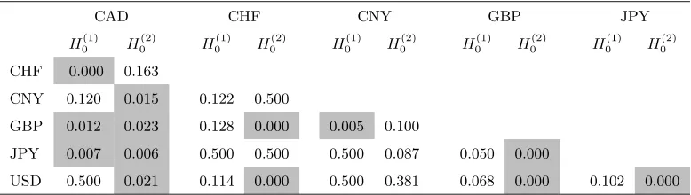
Table 5.For each pair of exchange rates:p-values of the tests of the null hypothesesH0(1)andH0(2) implied by the bivariate BEKK-GARCH(1,1) model. Gray cells containp-values less than 2.5%.
CAD CHF CNY GBP JPY
H0(1) H (2)
0 H
(1)
0 H
(2)
0 H
(1)
0 H
(2)
0 H
(1)
0 H
(2)
0 H
(1)
0 H
(2) 0
CHF 0.000 0.163
CNY 0.120 0.015 0.122 0.500
GBP 0.012 0.023 0.128 0.000 0.005 0.100
JPY 0.007 0.006 0.500 0.500 0.500 0.087 0.050 0.000
[image:29.595.117.506.542.652.2]Filtered probability of Regime 1
Time
Probability
0 500 1000 1500 2000
0.0
0.2
0.4
0.6
0.8
1.0
Estimated volatility of the JPY exchance rate returns
Time
V
olatility
0 500 1000 1500 2000
0
5
10
20
30
Estimated volatility of the GBP exchance rate returns
Time
V
olatility
0 500 1000 1500 2000
0
2
4
6
8
10
[image:30.595.134.466.158.317.2]12
7. Conclusion
We studied a method allowing for simple estimation of MGARCH and SC models. Instead of applying the full QML to the whole set of parameters, which is often numerically inefficient (see Table 1) if not infeasible, we estimated the volatility parameters by QML equation-by-equation in a first step, and then used the volatility-standardized returns in a second step to estimate the conditional correlation matrix. In contrast to other methods which have been proposed in the literature, this approach does not make strong a priori restrictions on the volatilities of the individual returns, which may be general functions of the past values of all returns.
Our aim was not only to develop an easily implementable MGARCH estimation pro-cedure, but also to derive asymptotic estimation results under mild assumptions on the observed process. The complexity of MGARCH specifications often make the asymptotic properties of the QMLE difficult to establish. By contrast, the simplicity of the proposed procedure allows for a rigorous analysis of asymptotic theory.
Moreover, our procedure is compatible with different assumptions on the conditional cor-relation matrix. The constant case was studied in details, and we obtained the joint asymp-totic distribution of the volatility and correlation parameters. Such results are amenable to different extensions, one of which was considered in the paper (i.e. the hidden Markov model for the correlation matrix). We also used our first step estimator to test the BEKK specification. Other extensions are left for future research.
Appendix
A. Technical assumptions
We make the following assumptions on the volatility function.
A2: for any real sequence (ei)i≥1, the function θ(k) 7→ σk(e1, e2, . . .;θ(k)) is continuous and there exists a measurable function K:R∞7→(0,∞)such that
|σk(e1, e2, . . .;θ(k))−σk(e1, e2, . . .;θ(0k))| ≤K(e1, . . .)kθ (k)
−θ(0k)k,
and
E K(ǫt−1,ǫt−2, . . .) σkt(θ(0k))
A3: there exists a neighborhoodV(θ(0k))of θ (k)
0 such that
E sup θ(k)∈V(θ(k)
0 )
σkt(θ(0k)) σkt(θ(k))
!2 <∞.
A4: we haveσkt(·)> ω for someω >0.
A5: we haveσkt(θ(0k)) =σkt(θ(k)) a.s. iff θ(k)=θ(0k).
The next assumption allows to show that initial values have no effect on the asymp-totic properties of the estimator of θ(0k). Let ∆kt(θ(k)) = ˜σkt(θ(k))−σkt(θ(k)), at =
supksupθ(k)∈Θ(k)|∆kt(θ(k))|. LetC andρbe generic constants with C >0and0< ρ <1.
The "constant"Cis allowed to depend on variables anterior to t= 0.
A6: We haveat≤Cρt, a.s.
To derive the asymptotic distribution of ˆθn, the following additional assumptions are considered.
A9: for any real sequence (ei)i≥1, the function θ(k)7→σk(e1, e2, . . .;θ(k)) has continuous second-order derivatives;
A10: there exists a neighborhoodV(θ(k) 0 )ofθ
(k)
0 such that
sup θ(k)∈V(θ(k)
0 )
1
σkt(θ(k))
∂σkt(θ(k)) ∂θ(k)
4(1+1
δ)
, sup θ(k)∈V(θ(k)
0 )
1
σkt(θ(k)) ∂2σ
kt(θ(k)) ∂θ(k)∂θ(k)′
2(1+1
δ)
,
sup θ(k)∈V(θ(k)
0 )
σkt(θ(0k)) σkt(θ(k))
4 ,
have finite expectations.
The next assumption is introduced to handle initial values.
A11: We have
bt:= sup k
sup θ(k)∈V(θ(k)
0 )
∂∆kt(θ(k)) ∂θ(k)
≤Cρ
t, a.s.
A12: Fork= 1, . . . , mand for anyx∈Rdk, we have:
x′∂σ 2 kt(θ
(k) 0 )
∂θ(k) = 0, a.s. ⇒ x= 0.
The next assumption is used in Theorem 3.2.
A10∗: there exists a neighborhoodV(θ(k) 0 )of θ
(k)
0 such that
sup θ(k)∈V(θ(k)
0 ) 1
σkt(θ(k))
∂σkt(θ(k)) ∂θ(k)
4 , sup θ(k)∈V(θ(k)
0 ) 1
σkt(θ(k)) ∂2σ
kt(θ(k)) ∂θ(k)∂θ(k)′
2 , sup θ(k)∈V(θ(k)
0 )
σkt(θ(0k)) σkt(θ(k))
4 ,
have finite expectations.
B. Proofs
B.1. Proof of Theorem 3.1
a) The strong consistency ofθˆ(nk) is a consequence of the following intermediate results:
i) lim
n→∞ sup
θ(k)∈Θ(k)|
Q(nk)(θ (k)
)−Q˜(nk)(θ (k)
)|= 0, a.s.,
ii)E|ℓk,1(θ(0k))|<∞, and ifθ(k)6=θ (k)
0 , Eℓk,1(θ(0k))<Eℓk,1(θ(k)), iii)any θ(k)6=θ0(k) has a neighborhoodV(θ(k))such that
lim inf
n→∞ θ∗∈infV(θ(k)) ˜
Q(nk)(θ ∗
)>lim sup
n→∞
˜
Q(nk)(θ (k) 0 ), a.s.
Because the proof follows along the same lines as the proof of Theorem 7.1 in Francq and Zakoïan (2010) we omit details. It is easy to see that i) follows from A4, A6 and the existence ofE|ǫkt|s. To show ii), first note that E η∗kt| Ftǫ−1
= 0. In view of (2.3), we thus have
Eℓkt(θ(k)) =E
(
σ2 kt(θ
(k) 0 )ηkt∗2 σ2
kt(θ
(k)) + logσ 2 kt(θ
(k)
) )
=Eσ
2 kt(θ
(k) 0 ) σ2
kt(θ
(k))+Elogσ 2 kt(θ
(k)
)<∞.
SinceElogσ2
sequenceinfθ
∗∈V(θ(k))∩θ(k)ℓkt(θ∗), which is strictly stationary and ergodic under A1and
admits an expectation in(−∞,∞].
b) Now we turn to the proof of the asymptotic normality. Define ℓ˜kt as ℓkt, with σkt replaced byσ˜kt. The proof relies on a set of preliminary results.
i)E
∂ℓkt(θ(0k)) ∂θ(k)
∂ℓkt(θ(0k)) ∂θ(k)′
<∞, E
∂2ℓ kt(θ(0k)) ∂θ(k)∂θ(k)′
<∞,
ii)There exists a neighbourhoodV(θ0(k))ofθ(0k) such that
sup θ(k)∈V(θ(k)
0 ) 1 √n n X t=1
∂ℓkt(θ(k)) ∂θ(k) −
∂ℓ˜kt(θ(k)) ∂θ(k)
→0,
iii) 1
n n
X
t=1 ∂2ℓ
kt(θ(nk))
∂θ(k)∂θ(k)′ →Jkk, a.s. for anyθ (k)
n betweenθˆ (k) n andθ
(k) 0 ,
iv)Jkk is non singular,
v) √1n n
X
t=1
∂ℓkt(θ(0k)) ∂θ(k)
L
→ N(0,Ikk).
Note that
∂ℓkt(θ(k)) ∂θ(k) =
1− ǫ
2 kt σ2 kt 2 σkt ∂σkt ∂θ(k)
,
∂2ℓ kt(θ(k)) ∂θ(k)∂θ(k)′ =
1− ǫ
2 kt σ2 kt 2 σkt ∂2σ
kt ∂θ(k)∂θ(k)′
+2 3ǫ 2 kt σ2 kt − 1 1 σkt ∂σkt ∂θ(k)
1
σkt ∂σkt ∂θ(k)′
.
Letk · kr denote theLr norm, forr≥1, on the space of real random variables. We have, by the Hölder inequality,
1−η∗2kt
1
σkt ∂σkt ∂θ(k)(θ
(k) 0 ) 2
≤ 1−ηkt∗2
2(δ+1)
1 σkt ∂σkt ∂θ(k)(θ
(k) 0 )
2(1+1/δ) ,
which is finite by Assumptions A8 and A10. The first result in i) follows. The second result can be shown similarly.
Now, turning to ii), we have
∂ℓkt(θ(k)) ∂θ(k) −
∂ℓ˜kt(θ(k)) ∂θ(k)
= ǫ2 kt ˜ σ2 kt − ǫ 2 kt σ2 kt 2 σkt ∂σkt ∂θ(k)
+ 2
1− ǫ
2 kt ˜ σ2 kt 1
σkt −
1 ˜
σkt
∂σkt ∂θ(k)
+
1− ǫ 2 kt ˜ σ2 kt 2 ˜ σkt ∂σkt ∂θ(k) −
∂σ˜kt ∂θ(k)
where
ut= (1 +ηkt∗2)
1 + sup
θ(k)∈V(θ(k) 0 ) 1 σkt ∂σkt ∂θ(k)(θ
(k)
)
1 + sup
θ(k)∈V(θ(k) 0 )
σkt(θ(0k)) σkt(θ(k))
2 ,
as a consequence of Assumptions A4, A6andA11. We haveE|ut|<∞by Assumptions A8andA10, and using the Cauchy-Schwarz inequality. ThusCPnt=1ρtu
tis bounded a.s., which entails ii).
To prove iii), by Exercise 7.9 in Francq and Zakoïan (2010), it will be sufficient to establish that for anyε >0, there exists a neighborhoodV(θ0(k))ofθ(0k)such that
lim n→∞ 1 n n X t=1 sup θ(k)∈V(θ(k)
0 )
∂2ℓ kt(θ(k)) ∂θ(k)∂θ(k)′ −
∂2ℓ kt(θ(0k)) ∂θ(k)∂θ(k)′
≤ε a.s. (B.2)
By the ergodic theorem, the limit in the left-hand side is equal to
E sup θ(k)∈V(θ(k)
0 )
∂2ℓ kt(θ(k)) ∂θ(k)∂θ(k)′ −
∂2ℓ kt(θ(0k)) ∂θ(k)∂θ(k)′
provided that this expectation is finite. In view of A9, the conclusion will follow by the dominated convergence theorem: the latter expectation tends to zero when the neighbor-hoodV(θ(0k))shrinks to the singleton{θ(0k)}.To complete the proof of iii), it thus remains to show that
E sup θ(k)∈V(θ(k)
0 )
∂2ℓ kt(θ(k)) ∂θ(k)∂θ(k)′
<∞. (B.3)
Let us consider the first product in the right-hand side of (B.1)). We have, by the Hölder inequality,
E sup θ(k)∈V(θ(k)
0 )
1− ǫ 2 kt σ2 kt 1 σkt ∂2σ
kt ∂θ(k)∂θ(k)′
≤
1 +kη
∗2 ktk2(1+δ)
θ(k)∈V(supθ(k) 0 )
σ2kt(θ (k) 0 ) σ2
kt(θ (k)
) 2
θ(k)∈V(supθ(k) 0 ) 1 σkt
∂2σkt ∂θ(k)∂θ(k)′(θ
(k)
)
2(1+1/δ) ,
which is finite by AssumptionsA8andA10. The second product in the right-hand side of (B.1)) can be handled similarly. Thus iii) is established.
The invertibility ofJkk is a straightforward consequence ofA12. Now
1
√n n
X
t=1
∂ℓkt(θ(0k)) ∂θ(k) =
1
√n n
X
t=1
and v) follows from the Central Limit Theorem of Billingsley (1961) for ergodic, stationary and square integrable martingale differences. Indeed, the square integrability follows again from the Cauchy-Schwarz inequality,
E {1−η∗2
kt}2kdktd′ktk
≤ k(1−η∗2
kt)2k1+δkdktd′ktk1+1/δ, and Assumptions A8 and A10. Moreover, (η∗
t) is strictly stationary and ergodic as a function of the process(ǫt).
We are now in a position to complete the proof of Theorem 3.1. Since θˆ(nk) converges to θ(0k), which stands in the interior of the parameter space by A7, the derivative of the criterion Q˜(nk) is equal to zero at θˆ
(k)
n . In view of point ii), we thus have by a Taylor expansion ofQ(nk) atθ(0k),
√
nˆθ(nk)−θ (k) 0
oP(1)
= − 1
n n
X
t=1 ∂2ℓ
kt(θ∗(ijk)) ∂θ(ik)∂θ
(k) j !−1 1 √n n X t=1 ∂ ∂θ(k)ℓkt(θ
(k) 0 )
where theθ∗(ijk)’s are betweenθˆn(k) andθ(0k). The conclusion follows from the intermediate
results i)-v). ✷
B.2. Proof of the result of Section 3.2
We have
∂lt(θ(1)) ∂θ(1) =
1− 1
1−ρ2 0
ǫ1t σ1t −
ρ0ǫ2t σ2t ǫ1t σ1t 2 σ1t ∂σ1t ∂θ(1) ,
∂2l t(θ(1))
∂θ(1)∂θ(1)′ = −
1 1−ρ2
0
−2ǫ1t
σ1t
+ρ0ǫ2t σ2t ǫ1t σ1t 2 σ2 1t ∂σ1t ∂θ(1) ∂σ1t ∂θ(1)′
,
+
1− 1
1−ρ2 0
ǫ1t σ1t−
ρ0ǫ2t σ2t ǫ1t σ1t ∂ ∂θ(1)′
2 σ1t ∂σ1t ∂θ(1) . Hence
∂lt(θ(1)0 ) ∂θ(1) =
1−1 1
−ρ2 0
(η1∗t−ρ0η2∗t)η1∗t
2 σ1t ∂σ1t ∂θ(1) ,
∂2lt(θ(1)0 )
∂θ(1)∂θ(1)′ = − 1 1−ρ2
0{−
2η∗1t+ρ0η∗2t}η1∗t
2 σ2 1t ∂σ1t ∂θ(1) ∂σ1t ∂θ(1)′
.
We thus have
Var
(
∂lt(θ(1)0 ) ∂θ(1) ) = ζE 4 σ2 1t ∂σ1t ∂θ(1) ∂σ1t ∂θ(1)′(θ
(1) 0 ) , E ∂ 2l
t(θ(1)0 ) ∂θ(1)∂θ(1)′
!
= 2−ρ
2 0
1−ρ2 0 E 2 σ2 1t ∂σ1t ∂θ(1) ∂σ1t ∂θ(1)′(θ
(1) 0 )