Solar coronal stability problems

Ian S. Hardie

A Thesis Submitted for the Degree of PhD

at the

University of St Andrews

1993

Full metadata for this item is available in

St Andrews Research Repository

at:

http://research-repository.st-andrews.ac.uk/

Please use this identifier to cite or link to this item:

http://hdl.handle.net/10023/14090

Ian S. Hardie

Thesis subm itted for the degree of D octor of Philosophy of the Uni­

versity of St. Andrews

All rights reserved

INFORMATION TO ALL USERS

The quality of this reproduction is dependent upon the quality of the copy submitted.

In the unlikely event that the author did not send a com plete manuscript and there are missing pages, these will be noted. Also, if material had to be removed,

a note will indicate the deletion.

uest

ProQuest 10167376

Published by ProQuest LLO (2017). Copyright of the Dissertation is held by the Author.

All rights reserved.

This work is protected against unauthorized copying under Title 17, United States C ode Microform Edition © ProQuest LLO.

ProQuest LLO.

789 East Eisenhower Parkway P.Q. Box 1346

1

A b stra ct

Magnetohydrodynamic stability theory provides a powerful tool for understand­ ing and testing hypothesized mathem atical and physical models of observed phenom­ ena on the surface of the Sun. In this thesis, the problem of applying the ‘correct’ boundary conditions at the photospheric/coronal interface used in modelling coronal arcades is tackled. Then some aspects of the stability of coronal loops and arcades are investigated using a Fourier truncated series approximation for the equation of motion.

The problem involving the boundary conditions has been the subject of a con­ troversy for the past decade with two principal conditions suggested, the ‘rigid-wall’ conditions where all perturbations vanish at the interface, and ‘flow-through’ con­ ditions where flows parallel to the equilibrium magnetic field take place.

By modelling the photosphere and corona as two different density regions and then varying the ratio of the densities of the two regions, growth rates and eigen­ functions of both ideal and resistive modes are investigated in order to follow the evolution of the modes as the density ratio is increased. In order to simplify the analysis, the 2-D equations are reduced to 1-D equations by taking a WKB ap­ proximation for the spatial variations across the field to give a localized ballooning approach with ordinary differential equations along the fieldlines.

111

D eclaration s

I, Ian Stuart Hardie, hereby certify th at this thesis has been composed by myself, that it is a record of my own work, and that it has not been accepted in partial or complete fulfilment of any other degree or professional qualification.

Signed; Date..(ft...

I was adm itted to the Faculty of Science of the University of St. Andrews under Ordinance General No. 12 on 1 October 1988 and as a candidate for the degree of Ph.D. on 1 October 1989.

Signed Date..!.^.'..?.

I hereby certify that the candidate has fulfilled the conditions of the Resolution and Regulations appropriate to the Degree of Ph.D.

In submitting this thesis to the University of St. Andrews I understand that I am giving permission for it to be made available for use in accordance with the regulations of the University Library for the time being in force, subject to any copyright vested in the work not being affected thereby. I also understand that the title and abstract will be published, and that a copy of the work may be made and supplied to any bona fide library or research worker.

I would like to thank everyone who has helped me in the creation of this thesis. Dr Alan Hood, my supervisor, who has guided me for the past few years, without his suggestions this thesis would not have been possible.

Also, everyone in the Solar Theory group and in the Department of M athematical and Computational Sciences including Colin D.C. Steele, Christopher Ridgway, Neil R. Strachan and Gordon Inverarity, the co-occupants of room 223.

Financial support was provided by S.E.R.C., the Science and Engineering Re­ search Council.

Finally, and most im portant of all, I would like to thank my parents, Stuart L.S. and Davina L.H. for their guidance, moral and financial support over the years since 1965, and my sisters, Grace, Hazel, Fiona and Shona for being there.

D ed ica tio n

C ontents

1 Introduction 1

1.1 Magnetohydrodynamics ... 1

1.2 MHD e q u a tio n s... 3

1.3 Basic MHD Plasma W av e s... 4

1.4 S ta b ility ... 7

1.5 Stability m o d e s ... 9

1.6 Coronal loops and a rc a d e s ...12

1.7 A Brief Review of Stability T h e o r y ...14

2 R esistive Ballooning Line-Tied Boundary Conditions 19 2.1 In tro d uctio n ... 19

2.2 Simple model of b o u n d a ry ...20

2.3 E q u a tio n s ... 22

2.4 Construction of the WKB solution ...26

2.5 Dispersion r e la tio n ...33

2.5.1 Uniform D e n s ity ...35

2.5.2 Infinite density l i m i t ... 37

2.6 General p ... 45

2.6.1 Ideal C a s e ...46

2.7 D iscussion... 53

3 Equilibrium and Equations of M otion for Coronal Loops 58 3.1 Intro d u ctio n ... 58

3.2 E q u ilib riu m ... 61

3.3 Linearized E q u a tio n s...66

3.4 M e th o d ...72

3.5 Field P r o f ile s ...73

4 Stability of lin e-tied coronal loops 80 4.1 Loop Profile 1 ...80

4.2 Loop Profile 2 ...93

4.3 Analytic profiles...101

4.4 Free e n e r g y ... 110

4.5 S u m m a r y ...I l l 5 Stability of coronal arcades 116 5.1 In tro d u ctio n ... 116

6 Discussion 123

References 125

Appendix A-Derivation of Resistive Ballooning Equations for Chapter 2 128

1.1 M agn etoh yd rod yn am ics

The Sun, like most of the universe, is a plasma. A plasma is often described in literature as an ionized gas but such a simple definition belies the many underlying complexities. Thus, electromagnetic effects are im portant in the description of the plasma on a macroscopic scale. The simplest model comprises combining Maxwell’s equations with the equations of fluid dynamics to give what is termed Magnetohy­ drodynamics. The MHD equations form a self-contained system of eight equations in eight primary variables (B, v, p, p) and are valid provided that flow velocities are small compared to the speed of light (u c).

Maxwell’s equations are

V X B = (1.1)

V X E = (1.2)

V . B = 0, (1.3)

V - E = ^ , (1.4)

where

B is magnetic induction, loosely described as magnetic field, E is the electric field,

p is coefficient of magnetic permeability, e is coefficient of electric permittivity.

Assuming typical lengthscales of L and time T, the ratio of the second term to the first term in equation (1.1) in order of magnitude, is given by

(1.5)

and equation (1.2) by

E / L % B /T . (1.6)

Using (1.6), (1.5) reduces to

(1.7) where v (= L jT ) is a typical plasma flow velocity.

Thus, for <C c^, the second term in equation (1.1) can be ignored, leaving

j = —V X B. (1.8)

p Writing Ohm’s Law as

j = <r(E + v x B ) , (1.9)

where a is the electric conductivity, states that the plasma current density is pro­ portional to the total electric field. Then, using equation (1.8), equations (1.2) and (1.9) are rewritten as

Defining the magnetic diffusivity as

and taking q to be constant, then equation (1.10) may be rewritten as

® = V X (v X B ) + )?V"B, (1.12)

The presence of the velocity term in the induction equation (1.12) indicates that the evolution of the magnetic field is coupled to the evolution of the plasma treated as a fluid.

1.2 M H D eq u ation s

The MHD equations used in this thesis are D v

p— = ” Vp + j x B , (1.13)

^ = V X (v X B) + TfV'B, (1.14)

+ p V - v = 0, (1.15)

Dt

D ( p \

7 — 1 \p '^ I a (1.16)

~ ~ + V • V is the time derivative following the fluid.

Equation (1.14) is the induction equation. The ratio of the second term , the adjec- tion term, to the third term, the diffusive term is known as the magnetic Reynolds number,

R n . = (1.1 7)

where L, v and p represent typical lengthscales, velocities and diffusivities in the plasma. In the solar corona, taking rj ~ (see Priest, 1982), T = 2 X lO^K, V = 10®ms“^, L = 3 X 10®m gives a value for Rm of 10^^.

Equation (1.15) is the mass conservation equation, and indicates that mass is not being created or destroyed in the region under consideration.

Equation (1.16) is the energy equation. Thermal conduction and radiative effects have been neglected from this equation. In the adiabatic limit, given by p = 0, p oc where 7, the ratio of specific heats, is usually taken to be 5/3, except when considering isothermal variations, when it is taken to be unity.

1.3 B asic M H D P la sm a W aves

Before investigating complex MHD problems, it is useful in a physical sense to determine the basic waves which propagate in a MHD plasma.

In order to keep the analysis simple, start with a unidirectional magnetic field infinite in extent with uniform background plasma pressure and density.

B = BqGz, (1.18)

P — Po, (1.20) To investigate the wave motions of this configuration linearize all quantities

A ( r , t ) - X o + A i ( r , t ) , (1.21)

where X \ (r, t) is a small order perturbation to the equilibrium quantities. Write the perturbation

= (1.22)

with

k = k±ey -f (1.23)

where the y-z plane has been chosen to coincide with the wavevector k.

Substituting expression (1.22) into the linearized ideal MHD equations from equations (1.13), (1.14), (1.15) and (1.16) with rj — 0

-%wpoV = - ik p i + j i X Bo, (1.24)

—iujBi = ik X (v X B o ), (1.25) —iupi 4- ipok • V = 0, (1.26) -poPi + 7PoPi = 0, (1.27) with

Ji = —k X B i, (1.28)

Substituting equations (1.25) to (1.29) into the equation of motion (1.24) and defin­ ing the Alfven speed and the acoustic speed c^,

' A ~’2 - - 5 - (1.30)

ppo

,2 _ 7P0 Po

c; — ^4- , (1.31)

gives

- k^v\) V = [(cl + kj_Vy + clk\\Vz] k - k\\v\ (^k±Vy + k^iVz) (1.32) The x-component of equation (1.32) gives the Alfven wave frequency

(1.33) The y and z components of equation (1.32) lead to the dispersion relation

(cj -I- -t- Pk^^clv\ ~ 0, (1.34)

with solution given by the fast and slow magnetoacoustic wave frequencies

(ca + [1 ± y / l - 4a2] , (1.35)

with

For localized modes with k^\ « kx, kx —> 00, expanding (1.35)

a-3^)

ujj = k l (cl 4- v l) - ^11 21 ^2' + " ’ ’ (1-^^)

'-'s '

Introduction 7

1.4 S ta b ility

Stability theory is very im portant in relation to observed phenomena on the Sun. Any model suggested to explain solar phenomena such as coronal loop and arcade structures and prominence models must be tested for stability. If the model is found to be unstable on a timescale that is shorter than the observed lifetime, then it is not relevant and has to be rejected or modified by introducing either extra or different conditions. This may result in a closer correspondence to the observed phenomena. There are two main methods for testing stability. The normal mode approach is used in this thesis and will be described later. The energy method can be used for ideal MHD and is based on the fact that the sum of the total potential and kinetic energies is constant. A decrease in the potential energy will lead to an increase in the kinetic energy of the system representing an instability. By linearizing the perturbed ideal MHD equations an expression for the change in the potential energy (6W) is obtained. If any perturbation ^ gives a negative value for the change in potential energy, 6W^ then the system is unstable. A positive value of 8W means the system is stable to that particular perturbation (but possibly could still be unstable to other perturbations). The method was first used by Bernstein et ah, 1958. Take the force operator

the change in potential energy is the work done by the force to displace the plasma

SW = - ^ J ( - F ( ( ) d V , (1.40)

where the integration is over the volume of the plasma.

The advantage of the energy method is when seeking stability but not growth rates or oscillation frequencies, it is necessary to look for a perturbation which decreases the potential energy. More complicated equilibria can be investigated this way. Its drawback is it cannot be used when non-ideal effects are included such as resistivity or viscosity and the normal mode approach has to be used.

An equilibrium is assumed or derived from the magnetostatic equation ( ^ = 0)

i (V X B) X B = Vp. (1.41)

P

Many such equilibrium fields have been derived, and some of these fields have been named after the authors who first used them, such as the Gold-Hoyle field (Gold and Hoyle, 1960) and Anzer field (Anzer, 1968). The next step is to perturb the equilibrium field by introducing small variations as follows

p — Po + Pi

where Bo, po, po are equilibrium quantities, and B i, pi, pi, v are perturbed variables such that the ratios of equilibrium to perturbed quantities are large. The equations are linearized and time-dependence is assumed by looking for normal modes of the form / = f (r) a is termed the growth rate and if the real part of cr is positive then the equilibrium is linearly unstable since the perturbed variables will grow in time. Likewise, for <7 negative or purely imaginary, the equilibrium is stable. In many problems several or sometimes an infinite set of normal modes exist, and if one or more of these modes give a positive value for a, then the equilibrium is declared unstable. The normal mode method will be used throughout this thesis.

1.5 S ta b ility m od es

To illustrate the various instability modes, consider a cylindrically symmetric magnetic flux tube with an azimuthal magnetic field

B = Bg (r) eg, (1.43)

and pressure p from the equilibrium equation

^ {rBe) = 0. (1.44)

dr pr dr ^ '

Then Fourier analyse the linearized equations of motion in the poloidal and axial directions

(a)

XJ

(b)

(c)

(e)

(d)

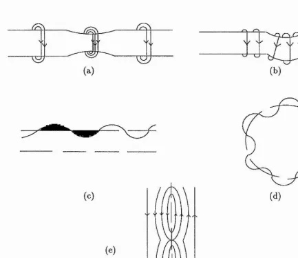
Figure 1.1: Diagrams of (a) Sausage mode (b) Kink mode (c) Interchange mode (d) Flute mode, and (e) Resistive tearing mode.

Introduction 11 the introduction of an axial component to the magnetic field as this gives rise to stabilizing magnetic tension forces at the constricted part of the flux tube.

Kink modes are obtained by setting m = 1. Physically a displacement of the flux tube perpendicular to the axis causes the magnetic field on the inside of the displaced tube to be concentrated and rarefied on the outer part of the displaced tube leading to the kink growing in size. The introduction of an axial component of the magnetic field gives a stabilizing component of magnetic tension.

Interchange or flute modes occur when two flux surfaces at different radii inter­ change. Interchange modes are driven by pressure gradients.

Ballooning modes are given by perturbations with long wavelengths along the magnetic field and short wavelengths across the magnetic field. The oscillations give rise to oppositely directed magnetic tension forces which combine with pressure gra­ dients to give regions of favourable and unfavourable curvature resulting in localized instabilities. Ballooning modes were used by Hood (1986) to investigate the effect of line-tying on flux tube stability. Line-tying converts a one dimensional problem into two dimensions. Making use of the ratio of the wavelength of the perturbations along the magnetic field to the wavelength of the perturbation across the equilibrium magnetic field, the equations are converted from two dimensional partial differen­ tial equations to one dimensional ordinary differential equations along the magnetic fieldlines which are easier to solve.

mag-netic fields. The fieldlines reconnect to form magmag-netic islands by tearing along the interface separating the two opposite magnetic fields. If this change in topology leads to a lower potential energy state a tearing instability occurs.

1.6 C oronal loop s and arcades

Observations indicate that much of the plasma in the corona of the Sun is in the form of loops. The loops are believed to trace out lines of force of the magnetic field emerging from beneath the photosphere. A study of loops can give a physical insight into the structure of the solar magnetic field. Coronal loops have been divided into two categories, ‘cooP loops with temperatures ranging from 20000 — 1 x 10® K and ‘hot’ loops with temperatures greater than 1 x 10® K. Active region cool loop systems can last for up to 5-6 hours. W idths vary from 300-2000 km and heights from 40000-50000 km. Active region hot loop systems last up to several days with widths from 3000-12000 km and heights from 50 000-250 000 km (see Bray et. ah, 1991). The Alfven travel time of a loop is several minutes. Given the long observed lifetimes, coronal loops must be stable. Stability is applicable in explaining the long lifetimes of many phenomena such as prominences and flares. Prominences are coronal structures which have a typical tem perature 100 times less and density 100

times greater than surrounding coronal values. They are stable for up to 300 days (see Priest, 1988).

energy released by a flare (up to 10^® W, see Svestka, 1976) must come from the magnetic field since no other source of such large quantities of energy is available to drive the flare. Flares occur in the corona of the Sun and from observations, the magnetic field is thought to be in the form of either coronal loops or coronal arcades.

CORONA

(a)

P H O T O S P H E R E

P H O T O S P H E R E C O R O N A

(b)

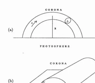
Figure 1.2: Diagrams of (a) Coronal loop (b) Coronal arcade.

several days in the form of electric currents in the non-potential field structure. At some point a loss of equilibrium or an instability occurs and there is a large release of energy over 20-30 minutes. This is known as a flare.

Flares have been divided into two main classes (see Priest,

1982):-(1) Small loop flares (or compact flares) with an energy release of 10^^ -10^^ W. Most flares are of this type. An individual loop appears to brighten without a substantial change of shape.

(2) Large two-ribbon flares with an energy release of up to 3 x 10^® W which generally occur in arcade structures. In this case there is a substantial restructuring and simplification of the field.

It is therefore im portant to investigate stability in relation to both loop and arcade structures.

1.7 A B r ief R ev iew o f S ta b ility T h eory

However, he found that all force-free cylindrically symmetric fields were unstable to m = 1 kink modes. This suggested that the flare energy could not be stored in the corona.

Raadu (1972) realized that the magnetic field is strongly stabilized by the ex­ tremely dense photosphere. To simulate the photosphere he proposed that the mag­ netic footpoints are anchored by line-tying due to the high inertia of the photospheric plasma. Thus, he argued that coronal disturbances must vanish at the photosphere, so that

a = 0, (1.46)

there. Since he only considered force-free fields and used the energy method, it is only the perpendicular displacement, (perpendicular to the equilibrium magnetic field), that enters the analysis. The inclusion of a finite gas pressure introduces the parallel component of the displacement and the boundary conditions regarding this component have been the subject of some debate.

Hood and Priest (1979) included a radial pressure gradient but restricted their choice of displacements so that

(|| = 0. (1.47)

Nonetheless, they showed that kink instabilities were present when the loop was sufficiently twisted. In addition, they proved that force-free loops were stable if the twist, $ = LBe/rBz^ was less than 27t.

ity (or equivalently the displacement) and suggested that this need not vanish but should merely satisfy conditions that preserved the total energy of the corona. For a loop they selected the flow-through conditions

= 0, at z=0,L

^11 (0) = ^11 (^) ’ (1.48)

These conditions simplify the manipulation of the energy integral and allow for in­ compressible displacements while still conserving the total energy. However, Rosner et al (1986) and Cargill et al (1986) have argued, on basis of timescales and physical arguments, that equation (1.48) is unlikely to be realized in practice since it as­ sumes that the photosphere can respond quickly to coronal perturbations and that it requires one end of the loop to ‘know’ what is happening at the other end simul­ taneously. Nonetheless, because the how-through conditions allow the elimination of a positive term in the energy integral, stability obtained using equation (1.48) guarantees stability for the ‘rigid-wall’ conditions.

in response to coronal motion. However, his analysis breaks down when the growth rate approaches marginal stability and \ppcr^\ is no longer large.

W hen instabilities evolve on a slower timescale, the situation may change. For example. Hood, Van der Linden and Goossens (1989) investigated therm al (or ra­ diative) instabilities and they found that substantial flow across the photospheric boundary was possible when the growth rate was sufficiently small. Cargill and Hood (1989) in their investigation of thermal instabilities in a sheared magnetic field have argued that a variety of thermal and magnetic boundary conditions should be used until the realistic conditions are proved.

discretization.

Hassam (1989) has cast doubt on the applicability of line-tying in stabilizing the tearing mode. He argues that the tearing mode evolves so slowly that there is plenty of time for the photospheric flows to develop. However, the instability he considers appears to be driven down in the photosphere whereas it is im portant to see the effect of disturbances initiated in the corona.

ditions

2.1 In tro d u ctio n

In this chapter the form of the boundary conditions at the coronal/photospheric interface is investigated. The growth rates and eigenfunctions of both ideal and resistive modes are investigated as the photospheric to coronal density ratio and resistivity are varied.

Firstly a simple model of a transverse wave on a two density string is considered in order to gain an idea of a sharp boundary between corona and photosphere in section 2.2. Then a model equilibrium and the stability equations that are used in section 2.3 are developed. Section 2.4 describes the construction of a normal mode from the ballooning approach and how plots of growth rate against radius should be interpreted. In the next section, the general dispersion relation is given and several limits are investigated analytically that provide bounds for the subsequent more general situations. Finally, section 2.6 presents the solutions of the dispersion relation for general density ratio and resistivity values.

'f ■V.

Resistive Ballooning Line-Tied Boundary Conditions 20 parallel to the magnetic field (see Connor et ah, 1979) since this reduces the energy required to overcome magnetic tension.

Taking a WKB approximation for the spatial variations across the field converts the MHD equations from a set of partial differential equations to a set of ordinary & differential equations with derivatives along the magnetic field.

In order to simplify the analysis, we consider an azimuthal magnetic field so that the derivatives are with respect to the azimuthal component.

2.2 S im p le m o d el o f boundary

In this section, a simple model of line-tying of a transverse wave on an elastic string of two different densities is considered.

Represent the displacement of the string on either side of the change in density by yi and p2 where

“ ^incident ^reflected) (^*1)

^2 — ^transmitted? (2.2)

where

2/incident = (2.3)

2/reflected = A e ^ "("« -* ), (2.4)

^transm itted

^reflected

Figure 2.1: Diagram showing an incident wave transm itting and reflecting across a boundary.

Since the string is continuous, yi = y2 for all t. Also the slopes d y i/d x = dy2/d x

for all t. The two boundary conditions imply

which have solution

Ai -]r Ar —

k\ (—A* + Ar) = —k2At,

k ] + k A ' A, = k\

4-(2.6)

(2.7)

(2.8)

Representing region 1 by the corona and region 2 by the photosphere and taking a constant magnetic field and a density ratio of 10®, then an Alfven wave has velocity (see Hood, 1992)

giving

- 1 4 - ^ / ^

Ar = j ^ A i =

-0.9998A ,

(2.12)

2x /

-At = ■ V ' A- = 1.9998 X 10~*Ai, (2.13) Thus a disturbance initiated in the corona is essentially totally reflected at the boundary with the photosphere. From expressions (2.3) and (2.4), the perpendicular velocity components of the wave will vanish at the interface.

2.3 E quations

The magnetohydrodynamic equations considered are

p - ^ = “ Vp + j x B , D v_{D t} (2.14)

+ V • (fv) = 0, (2.15)

® = V x ( v x B ) + ,,V"B, (2.16)

V • B = 0, (2.17)

pDp

where the momentum equation (2.14) consists of forces due to a pressure gradient and a Lorentz force, the induction equation (2.16) involves a uniform resistivity, and (2.18) is the energy equation with ohmic heating included.

We will consider an arcade consisting of a cylindrically symmetric azimuthal magnetic field. Be, and gas pressure, p, that are functions of r, but with a density, p, that is a function of r and Ô. The photosphere and corona are taken as two distinct regions of densities pp and pc, separated by a sharp transition region at 0 = ±7t /2. The idea is to see how the amplitude of the eigenfunction at ^ = ±7t/2 and the growth rate respond to changes in the density ratio Pp/Pc for various values of the dimensionless resistivity param eter p. The plasma beta, in such a model, is larger than typical solar coronal values but the emphasis here is to see how both stable and unstable modes are modified by the density ratio. To produce a ballooning instability requires a ^ oi order unity, since the instability is driven by an adverse pressure gradient.

The equilibrium equation is given by

dr UP A

2

B e ‘

(2.19)

Linearizing about this basic state and taking all perturbed quantities of the form equations (2.14) to (2.18) reduce to

Pqctvi = —Vpi 4— (V X B i) X Bo 4— (V x Bo) x B i, (2.20a)

p p

<tBi = V X (vi X Bo) + ??V^Bi, (2.20c)

V • B i = 0, (2.204

crpi + Vi • Vpo = - jp o V • vi + 2 (7 - 1) T/jo- (V X B i ) . (2.20e) To simplify these equations further, we make the ballooning approximation and take a WKB approximation for the spatial variations across the field, namely / (0) where n 1 is the ratio of equilibrium to perturbation length scales. The ohmic heating term in equation (2.20e), of order pn ‘drops out’ by comparison with the resistive term in equation (2.20c), of order pn? which is of order unity (see Appendix A). From the leading order equation we find that (ppi-L BoBie) — 0 (1 /n ) (see Hood et.al. 1989). Equations (2.20a) to (2.20e) reduce to

1dvie

r dO + Vir + lP pB e‘ Be‘

P — + — Pi - ppO-Pvir = 0, r do r

B) dvir

ftpi = 0, (2.21a)

(2.215)

(2.21c)

(2 .2 1 4

r de ~ Bir - 0.

where = 1 -f- {S*Ÿ is the square of the wave vector. Eliminating pi from equa­ tion (2.21c) using (2.21a) and differentiating (2.21d) with respect to 0 to eliminate dBir/d0 gives

(o- + (7/ip + Be^) p(^ r k

-\-2Bq7p 4- rjp p p 4-, rjn^k'^'ypppar'^k^

Vir = 0, (2.21e)

Similarly, eliminating pi from equation (2.21b) using the derivative of (2.21a) with respect to $, and (2.21d) to eliminate Bir gives

(cr + pn^k'^^ — ((J 4- pri^k'^^ [{^UP 4- Be^^ cr4- pn^A:^7pp] rpavie dvir

4-r

2Bg^7P (<T 4- pn^fc^)

4- pn^k'^p'Be^ = 0, (2.21/ )

Thus, the stability equations reduce to two coupled second order O.D.E.’s. To illustrate the ideas, we will use the example equilibrium

B = Bo

L°’ 1 + ,0

P with

2 /: (l4 -r4 ^

Bo" p" p (1 4- r^)"

since the results for ideal MHD are already known (Hood, 1986). The asterisk will be omitted, and isothermal disturbances, with 7 as unity, are taken for simplicity. Equations (2.21e) and (2.21f) reduce to

[(1 + 2r^) (7 4- — 2 (a 4- dvie

_de

Uir — 0, - (a 4- I 4- (l 4- 2r") pa^k^ + •qn^k'^pcr

(1 + r") (<r + W k ' ^ ) ^ + 2 [(1 + r') <r + (l - r')] ^

— (l + [(l + cr + (cr -f pcrv^Q —0. (2.226) In the ideal limit, yri^k'^ = 0, with k“^ = 1, equations (2.22a) and (2.22b) reduce to those of Hood (1986).

Since in each region, all coefficients are independent of 0, we take vir,vie of the form so that a fourth order equation in m is obtained

— + 2 (l + r") pa^k^ + 2rjn‘^P pa

1 r ^ 4 + — 4r^

+

m

(o- + ^ + (l + 2r^) pcr^A;" + yn^k'^po­ or in terms of k^ as

pn^p"cr^ [(l -f 2r^) cr + pn^]

4- [m'* 4- 2 ( l 4- m ^ p c r ^ + ( l + 2r^) p^cr^] A:

= 0, (2.23a)

-\-yn^por 2m^ 4- per' 4r" 1

4-r^po-^] = 0, (2.236)

Thus, there are four roots for m in each region, 4zmi, ± m2 in the corona and dbms, ± m4 in the photosphere.

2.4 C on stru ction o f th e W K B so lu tion

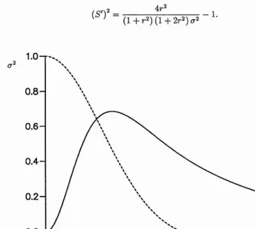
set S'{r) = 0 and obtain as a function of radius. This is shown in figure 2.2 for m = 0 and m = 1. The problem is how to interpret this figure in terms of actual normal modes. To do this we consider first the m = 0 mode. Equation (2.23b) then defines the radial wavenumber as a function of r and cr^ as

4^2

/ \ 2

( y ) _{(1 + r^) (1 + 2r^)} 1. (2.24)

.2

<T

0.8

0

.

2

-0.0

0.0

0.5

1.0

1.5

2.0

2.5

3.0

Figure 2.2: Square of the growth rate, cr^, as a function of the radial coordinate, r, in the uniform density ideal approximation, with poloidal wavenumbers, m = 0

(solid curve) and m = I (dashed curve).

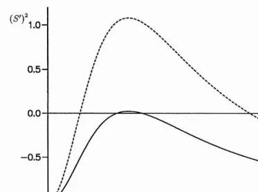
evanescent where (5')^ is negative and oscillatory where (S')^ is positive.

0.5-0.0

0.5

0.0

0.5

1.0

1.5

2.0

2.5

Figure 2.3: The radial wavenumber (S')^ as a function of radius, r, with the square of the growth rate given by cr^ = 0.67 (solid curve) and = 0.33 (dashed curve).

In the neighbourhood of (5')^ = 0 there is a turning point and the solutions on either side of this point can be connected using Airy functions. Having obtained the growth rate is determined by requiring that the oscillatory part of the solu­ tion has the “correct” number of oscillations to match onto the evanescent solutions. This generates a Bohr-Sommerfeld condition of the form

where M is the number of radial nodes, a is a number of order unity and a, b are the zeros of S'{r). cr^ is then adjusted until equation (2.25) is satisfied. An alternative way of using equation (2.25) is to specify evaluate the integral on the left hand side of (2.25) and then determine the value of n. As long as n >> 1 we have a valid solution. The actual value of a is determined by treating the turning points and boundary conditions in detail but if a is not too close to zero a is approximately 1/ 2.

The link between the WKB approach and the standard normal mode approach can be seen by studying the Hain-Lust equation (Goedbloed, 1983). For the uniform, in the $ direction, density case, the linearized ideal MHD equations can be reduced to one 2^^ order differential equation for the radial velocity, the Hain-Liist equation, for variations of the form f(r)exY>(i7nO-{-inz-{-o-t), that in the limit of large n reduces to (m = 0)

d r 1 / 2(7^ \ d X

7^‘^ dr \ r { I r'^Ÿ \ (1 + 2r^) / dr

+ + (1 + + 2r^) + ^ ^

where X = rvr.

Hence, to leading order the Hain-Liist equation becomes

g -

( « I

by replacing (5')^ by — 1/n^ d^/dr^ from equation (2.24) we can in fact recover the leading order differential equation, except for the first derivative term. The first derivative however, is only of importance near r = 0 when n is large (ie for n r < 1). Notice that correction terms in equation (2.26a) remain asymptotically small even in the neighbourhood of the zeros of S'(r). If S'(a) — 0, setting

a; = (r — a) (2.27a)

in equation (2.26a) generates Airy’s equation in the form

^ + C x X = O (n-2/^) , (2.276)

where C = 2(1 — 2a^) /a (1 -f a^) (1 + 2a^). Neglecting the corrections of O

this is equivalent to the Airy’s equation generated direct from equation (2.24). Therefore the equation derived from (2.24) agrees with the leading order behaviour of the Hain-Liist equation, (2.26a).

The behaviour of the m = 1 mode is slightly different. From figure 2.2 it is seen that (7 is a monotonically decreasing function of radius. This means that S'(r) = 0 at only one radius, r=c, say. Hence we have a one turning point problem. For r < c the eigenfunction is oscillatory and for r > c evanescent. Matching the two solutions, through Airy’s equation, the WKB expression for the eigenvalue becomes

n

J

In deriving (2.28a) it has been assumed that the eigenfunction is zero at r = 0. Notice that, again, the differential equation derived from (2.28b) agrees with the leading behaviour of the Hain-Liist equation, for large n, except near r = 0 (nr < 1). Table 2.1 illustrates the above relationships for the growth rate.

n M Hain-Liist Ballooning Integral

10 0 0.7731 0.7837 0.7832

10 4 0.5565 0.5614 0.5612

m= 0 30 0 0.8114 0.8126 0.8126

30 4 0.7078 0.7087 0.7087

10 0 0.9152 0.8584 0.8571

m = l 10 4 0.3139 0.2760 0.2756

30 0 0.9687 0.9509 0.9507

30 4 0.7300 0,7164 0.7163

Table 2.1: Values of the growth rate obtained numerically using Hain-Liist, Balloon­ ing and integral equations for the ideal uniform density m = 0 and m = 1 modes. M is the number of internal radial nodes.

from the differential equations generated from equations (2.24) and (2.28b). The “integral” column gives cr when using equations (2.25) and (2.28a).

Now we are in a position to interpret figure 2.2. Basically, the curve shows all the possible values for the growth rate. The radius (for a given value of cr) gives the location at which the eigenfunction changes its character from exponential to oscillatory (or vice versa). However, for every value of a given by figure 2.2 there is a possible normal mode that depends on the value of n (as long as n is large) and the number of nodes.

The inclusion of resistivity does not radically alter the above approach. Neglect­ ing the root corresponding to pure diffusion in the derivation of (2.23a), it is clearly seen that the ballooning approach generates a 4*^ order differential equation

1

d 0 ^ ~ ¥ -4r^

d?v + 2 (l 4- 4- 2'qn'^k'^pa

pa'^k'^4- r}n^Ppa (cr -j- —0, (2.29)

+

Again this equation agrees with the leading order behaviour, for large n, of the actual linearized equations away from the origin (ie. the equations are valid for nr %$> 1). Factorising into a pair of 2”®* order equations reveals that one factor is simply the ideal equation modified by resistivity whereas the other equation admits the possibility of a new resistive mode. For eadh of these two equations, normal mode solutions can be constructed in the manner described above.

values for the growth rate, cr, by setting {S'Y = 0 and plotting cr as a function of r. Given a value for cr, the above analysis shows that there is a normal mode solution that depends on the value of n and the number of radial nodes. The radius at which cr attains this value corresponds to the radius at which the nature of the solution changes from oscillatory to evanescent (or vice versa).

When the density is non-uniform, in the 0 direction, the same approach can, in principle, be carried out but the actual derivation of the normal mode is substantially more complicated. Instead we select a typical radius and see the effect on this value for the growth rate as the photospheric density is varied. Generally speaking the variation of cr is similar at all radii. However, following this approach we are unable to follow the same normal mode as we have no guarantee that n and the number of radial modes will remain the same.

In section 2.5 we begin by constructing the general dispersion relation before dis­ cussing the two extreme limits of uniform density and infinite photospheric density. Then the way in which one solution evolves into the other is investigated by varying the photospheric density in section 2.6.

2.5 D isp ersio n relation

Consider initially even modes, about ^ = 0, for Vir and odd modes for which we shall write as Vr and ug.

V r p = c C O S m 3 (tT — Û ) ~ h dCOS m 4 (tt —

0

V&C = Asinm iO B sinmg^,

Vûp = C sin m3{tc ~ 0) D sin (tt — ,

(2.306) (2.30c) (2 .3 0 4

where subscript p refers to the photospheric, and c refers to the coronal regions. Equation (2.22) is used to write A, J5, C and D in terms of a, 6, c and d and matching (2.30a) to (2.30d) across the coronal/ photospheric boundary, 0 =

±

/

,

1 1

" h Z ta n m if tan m g f tan mg^ ta n m4^ mi

E , - m lF

m2

Er m \F

m3

Ep — m^F

m4

m ita n m if mg tan m2 § m3 tan m3 ^

En — TtÎaF

m.4 ta n m4f

0,

where

Ec. = —— En = - ^

—4^.2

1 -f —4?'^

-f (1 + 2r^) + lyn^pccr + (1 + 2r^) + Tfn^ppcr

(2.31a)

(2.316)

(2.31c)

and m i, mg, m3 and m^ are solutions to (2.23a).

This dispersion relation is now solved analytically for two special density limits.

2.5.1 Uniform D ensity

In this extreme we take pp = Pc = 1, and we have to solve equation (2.23) with the condition that m is an integer to satisfy the periodicity of the disturbances. Several simple cases, for particular values of the radius, are described. This is equivalent to a ballooning mode analysis of a Z-pinch.

Analysing equation (2.23a), with (S 'Y = 0, = 1, it is clear that the only unstable modes occur for m = 0 and m = 1. The behaviour of cr as varies is typified by the particular radius r = 1. In this case, equation (2.23a) factorizes to

[m^ + (T (cr + 7/n^)] [m^ — 2 + cr (3cr + — G, (2.32)

giving the solutions

cr = — ± — j Inn'* ) —4m' (2.33a)

r]n^ , 1

MG"')

whereas the stable root has an increased damping rate. The two damped oscillatory slow modes become two damped real modes for rjn^ > 2. This point coincides with the damped Alfven mode only for r = 1. For r I there is no coincidence of 3 roots. The behaviour for other values of m is readily obtained from (2.33).

— 1

3

-4~

—5 —

6

1

2

0

3

4

5

6

2.5.2 Infinite density lim it

Taking ^ 1,

pp = p

\p<r\

E c - m i^ F 7T E c-rri2^F ^ tt

---tan m i— = --- tan m2—. (2.34)

mi 2 m2 2

where Ec and F are given by expressions (2.31), (see Velli and Hood, 1986), since if we represent the term in the row and column of the dispersion relation (2.31) by

Kij,

« 1 3 = O (1) « 1 4 = O (1) « 2 3 = O ( ( /> < t ) 2 ) « 2 4 =

o

« 3 3 =

o (pa) K34 - O

« 4 3 =

o

O

Hence the contribution from « 3 3 x «44 dominates all other product contributions

from columns 3 and 4. 2.5.2.1 small r

Before investigating the numerical solutions to the dispersion relation, it is in­ formative to analyse the behaviour of cr in the neighbourhood of the origin, r = 0. Through this approach the singular nature of the resistive problem and the actual number (and form) of the roots are clearly seen.

W ith r = 0, equation (2.23a) factorizes as

and taking rtm j, dzmg as solutions of equation (2.35), for small r, there is an infinity of solutions of the form

Tjn

m2 = m i 4- 2,

(2.36a)

(2.366) to first order, where m i and m2 are integer values in order to satisfy the dispersion

relation (2.34).

Using equations (2.36a) and (2.36b) and substituting integer values for m i, we obtain the small r perturbation expansions, in the following forms

13

cr — ± + .. .^ , r)n^ = 0,m i = 0,

<7 = ± i\/E ^1 — + .. .^ , Tjn'^ = 0, ?ni = 1, o- = + . . . , 7]n^ ^ 0, T]ri^ > r, mi = 0,

(2.37a)

(2.376) (2.37c)

a — — rjn + (—24

6(r}n^Ÿ^ ±

b2{r}n'^Ÿ

9{Tjn^y

2f]n'^

4 . . . , 7/72^7^0, 7/72^ ;> r ,mi = 0, (2.37d) The different forms for mi = 0, namely (2.37a) and (2.37c), illustrates the sin­ gular nature of the stability problem. Thus, the inclusion of resistivity may produce a pronounced effect when comparing with the ideal results.

Looking at any particular solution of equations (2.36a) and (2.36b) with mi / 0, then

o-{mag = ^ ^ (7 — (Jfcal i ifTiniag

and as rjn? increases, \(Timag\ reduces until {rfn’^Ÿ ~ = 0 when (Ximag = 0. Then, for {rjn^Ÿ ~ 4m im2 > 0, cr becomes purely real and negative. As oo, CF asymptotes to the values 0 and —T]n^.

2.5 .2.2 General r

Dispersion relation (2.34) together with the fourth order equation (2.23), have been solved numerically for different values of r and rfn^ and the results are now discussed. Consider first the infinite density limit.

0.4-1

0

.

2

-0.0

0.4

0.0

0.2

0.4

0.6

0.8

1.0

1.2

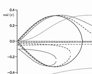
Figure 2.5a: Real component of the growth rate, cr, as a function of the radial

coordinate, r, in the infinite density ratio approximation in the ideal limit (solid curve), and also = 0.05, 0.1, 0.5 and 1.0 (dashed curves of decreasing length).

shorter dashes. In figure 2.5a, the solid curve shows the ideal Alfven modes are purely real for r < 0.9. For r > 0.9, the ideal Alfven modes are stable. Figure 2.5b clearly illustrates the region at which stable Alfven modes appear. In addition, the slow mode is stable for all values of r. Notice that in the region r > 0.9 the unstable mode is a purely real mode that owes its existence to resistivity. The allowable normal mode growth rates are similar to the ideal values but the radial extent (of the oscillatory part) of the eigenfunction is more extended. Two solutions of complex type exist for non-zero which merge and disappear at a value of ijn? less than 0.05. One of these two roots is tabulated below.

r}ri^ a

0.00 ( 0.00x10°, 0.2202)

0.01 ( 6 .1 3 x lO -\ 0.2188)

0.02 ( 8 .6 1 x lO - \ 0.2141)

0.03 ( 2 .8 4 x lO -\ 0.2050)

0.04 (-2 .0 1 x lQ -\ 0.1872)

Table 2.2: Values of the growth rate obtained for small rjn^ at r = 1.0. This solution merges with its complex conjugate pair and disappears for greater values of Tjn^.

One overstable and one damped oscillatory solutions for 7/n^ = 0.03 can be shown to exist. As i]n^ is increased, the solution with the smaller imaginary value

2.0-1 imag (<%)

1

0

0.5-0.0

—0.5--

1

0

-—

2

0

0.0

0.2

0.4

0.6

0.8

1.0

1.2

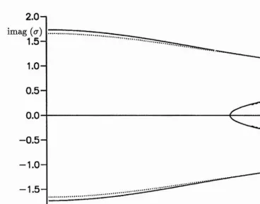
Figure 2.5b: Oscillatory component of the growth rate, cr, as a function of the radial coordinate, r, in the infinite density ratio approximation in the ideal limit (solid curve), and for = 0.5 and 1.0 (dashed curves of decreasing length).

dispersion relation (2.34) since F in (2.31c) is indeterminate.

cr

TfU

—

2

3

0

2

4

5

Figure 2.6: Growth rate, <t, as a function of Tjn^, in the infinite density ratio ap­ proximation with radial coordinate, r = 0.5. Solid curves correspond to the Alfven mode , dashed curves to the slow mode.

roots that coalesce and then reappear at a larger value of r/n^. This is identical to the points of coalescence at r = 0 which occur (at rjri^ = 0.08, 5.7) when the square root term in (2.37d) changes from real to imaginary and back to real again, as rjn^ is increased.

To apply the rigid wall line-tying conditions, the photospheric density must be sufficiently large that 1. Then starting at the ideal limit, rjn^ = 0, there are four fundamental roots to the dispersion relation, namely the real unstable and stable Alfven modes, and the purely imaginary slow modes. As increases the slow mode becomes damped with a damping rate of 7/n^/2, and the frequency is reduced until at rjn^ % 4.1 the frequency is zero and above this there are two real stable modes. The growth rate of the unstable Alfven mode is reduced but remains unstable. This is in contrast with the results found in Velli and Hood (1986). However, Velli and Hood investigated regions of ideal marginal stability given by r % 0.9 in figure 2.5, and in that region it is clear that resistivity increases the growth rate.

for ai = 0 and the real part of (2.34) is zero, (with ai = 0) at two distinct values of ar, giving the two roots. However, when r]n^ = 0.12, although the imaginary part of (2.34) is zero for ai — 0, the real part of (2.34) (with ai — 0) does not possess any zeros indicating there are no solutions to the dispersion relation.

When r = 1, the plasma is ideally stable and at rjn^ = 0, there are the 4 frequencies, the larger values of jcr^| correspond to the slow modes and the smaller values to the Alfven modes. As increases the slow modes are again damped with a rate proportional to r)n^/2. The purely real resistive ballooning mode, is clearly seen emanating from the origin and soon reaches a maximum value before slowly decreasing. Beyond rjn^ — 2.5, two real roots emerge.

2.6 G eneral

To proceed, equations (2.22a) and (2.22b) have been solved numerically using a fourth order Runga-Kutta-Merson method with density profile given by

1

P (1 + Pp) + (1 — pp) tanh A (2.38)

where A has been taken to be 1000 to give a steep density transition from /? = 1 to p = Pp as ^ is increased across the boundary ^ = 7t /2. A typical value of the radius is selected to illustrate the influence on the growth rates of increasing pp.

2.6.1 Ideal Case

Firstly, consider an ideal plasma. The values of r are selected as they are typical of the uniform and infinite density limits. At r = 0.5 and 1, the uniform density limit has both the kink and sausage modes unstable whereas there is only one unstable mode for r = 0.5 in the infinite density limit and there are no unstable roots at r = 1. For r = 2 only the sausage mode is unstable in the uniform density limit and there are no unstable roots in the infinite density limit. Thus these three values of r cover the different cases and we now consider how these ideal modes evolve as the photospheric density varies. The behaviour of a for r = 0.5, as pp varies is shown in figure 2.7a for the kink-type and sausage-type modes. The former tends to a finite value that is given by the infinite density value, whereas the latter tends to zero. The growth rate of the kink-type mode is given b y # ; % ctoo + for large p, whereas the sausage-type mode is given by <j w C2p~^^^. Notice that for the sausage

infinite density limit.

0,8

cr

0

6

0.4-0

2

0.0

1

5

10

50 100

500 1000

Figure 2.7a: Growth rate, cr, as a function of the density ratio, /?, with radial coordinate, r = 0.5, in the ideal limit. The infinite density ratio limit is shown as a dashed horizontal line. The kink-type mode is shown by a dashed curve, the sausage-type by a solid curve.

to 0 as /o increases indicating that there is a flow across the boundary. Using a normalisation of = 1 at (9 = 0, the relationship between velocity and density is shown in figure 2.7b. The eigenfunction for the kink-type mode, has a maximum at 0 = 0 and minimum at ^ = ±7t /2, whereas, for the sausage-type mode, it has a minimum at 0 = 0 and maximum at 0 = ±7r /2. Since, in the corona, the radial velocity has the form

5-1

V

3

-2

-50 100

500 1000

Vr = acos?ni0 + 6 cos m20 (2.39) this can be explained by a and b having the same sign for the kink-type mode, and opposite signs for the sausage mode. For r = 1.0, the sausage-type growth rate is larger in value than the kink-type growth rate, with both types of mode tending to

0 as p is increased. The amplitude of the kink-type velocity eigenfunctions tends to a finite non-zero limit and again the growth rate tends to 0 as p is increased. In contrast to r = 0.5, the sausage-type mode has a maximum at 0 = 0 and a minimum at 0 = ±7r /2, and the kink-type mode has a minimum at 0 = 0 and a maximum at 0 = ±7r /2. The growth rate of the sausage-type mode is given by <j % C2p“^/^ for large p, whereas the kink-type mode is given by <r « cip"^/^. Hence, the sausage mode satisfies rigid wall line-tying conditions but the kink mode, since |p<7^j is not large, does not.

For r = 2.0, there is no unstable kink-type mode since < 0 for r > a/3 - The

sausage-type growth rate is similar to the case r = 1.0 with a tending to 0 as p tends to 00. The growth rate is given by cr oc p“^/^.

with Hood (1986) that for large photospheric/coronal density ratios, the line-tying conditions are best simulated by taking all velocity amplitudes to be zero at the photospheric boundary.

2.6.2 non-zero

We now investigate how the growth rates are influenced by the inclusion of resistivity. Again 3 values of r are used as above.

0.8

0.7

cr

0.6-0.5 — 0.4 -0.3

0.2—

0.1

0.0

1 5 10 50 100 500 1000

Figure 2.8a; Growth rate, cr, as a function of the density ratio, p, with radial coordinate, r = 0.5, and — 0.5. The infinite density ratio limit is shown as a dashed horizontal line. The kink-type mode is shown by a dashed curve, the sausage-type by a solid curve.

case with the amplitude of the kink-type velocity eigenfunctions tending to zero as p is increased. Figure 2.8a shows the behaviour of the kink-type (dashed curve) and sausage-type (solid curve) growth rates as the photospheric density varies. Again, the former tends to a non-zero value given by the infinite density limit, whereas the latter tends to zero. However, the velocity eigenfunctions do not go to zero, since a contribution to the ballooning equations will come from the second order derivative of the perturbed magnetic field with respect to the poloidal angle, 0. This will introduce diffusive terms, which vary as rjpa^ into the two coupled second order ordinary differential equations for Vr and ve given by equations (2.22a) and (2.22b). The growth rate, cr, tends to a non-zero positive value as the density ratio, p tends to infinity, and -qpa will cease to be small compared to •qri^k'^ and so a small non-zero velocity will remain with an amplitude dependent on the diffusion timescale (see Velli, Einaudi and Hood, 1990).

The amplitude of the sausage-type eigenfunctions at 6 —

±

as p is increased for the resistive r = 0.5 case. However, since we are normalising the amplitude of the radial velocity eigenfunction to unity at 0 = 0, we have calculated Vr/{a b) from expression (2.41), and a-j-6 tends to zero as p is increased. Again, the sausage-type eigenfunction, has a minimum at 0 = 0 and maximum at 0 =

±

and p for •qn?' = 1.0, somewhere between the —1/3 and —1/2 values obtained for the ideal case.

300-,

V

250-200

-

150-100

5 0

-1

5

10

50 100

500 1000

Figure 2.8b: Radial (upper) and poloidal (lower) velocities at the photo­ spheric/ coronal boundary, 9 = 7t /2, for unstable modes corresponding to figure

2.8a.

eigenfunctions tends to zero as p is increased. As explained above, the velocity eigenfunctions do no go to zero but will tend to a small, non-zero, value dependent on the diffusion timescale with extra terms in the coupled ordinary differential equations due to the second order derivative of the perturbed magnetic field.

The amplitude of the kink-type radial velocity eigenfunction tends to a non-zero value, with the growth rate tending to 0 as p is increased. The kink-type growth rate, cr % cp“^, for r = 1.0, whereas the kink-type mode is non-existent for r = 2.0. The sausage-type growth rate varies approximately as for r = 1.0, p'n? — 0.5, and for the cases r = 1.0, 'qn^ = 1.0 and for r = 2.0, qn^ = 0.5 and 1.0, somewhere between the power values —1/3 and —1/2 obtained for the ideal case.

2.7 D iscu ssi

on

In this chapter, we have looked at the behaviour of both ideal and resistive ballooning modes as the photospheric to coronal density ratio, resistivity and radius are varied in order to investigate the correct form of the boundary conditions at the photosphere/corona interface.

adjusting the wavenumber n and the number of radial nodes. Choosing a particular value of r allows us to predict the influence of resistivity and the photospheric density on the behaviour of attainable normal modes. We have looked at a larger range of parameters than has previously been attem pted, with the resistivity parameter, qn^, extending beyond the maximum value of 10"^ used in Velli and Hood (1986) up to a value of 6.0, in order to follow the development of some of the modes as the resistivity is varied. Unless anomalous resistivity is used, such high values of qrt^ are unlikely to be achieved in the solar corona. Previous attention has been focused on a particular value of the radius. This chapter has shown that the effect of resistivity on unstable modes can be different depending on the value of the radius chosen. In the case of an infinite density ratio, resistivity decreases the growth rate for small r, whereas beyond ideal marginal stability, r = 0.9, resistivity causes an increase in the growth rate, the region investigated by Velli and Hood (1986). Our analysis has looked at small perturbations about a cylindrical magnetostatic equilibrium where the coronal and photospheric pressures and magnetic fields depend on the radius, and are independent of the poloidal angle, and toroidal z direction. The large wave-number, n, in the radial and z directions for the perturbed quantities, gives slow variations along the field lines but rapid variations across them.

the field lines. Hood (1986) investigated the ideal case with r = 0.5, and found that for the most unstable mode, the kink-type mode, the ‘rigid-wall’ conditions were the most appropriate as the density ratio becomes large. He also found the governing equation in the infinite-density ratio case when the corona becomes detached from the photosphere, indicating agreement with the ‘rigid-wall’ conditions. However, the density ratio is not infinite, but of the order of 10®, and it is not obvious that a large finite ratio should give similar results to an infinite ratio. This chapter has shown that there exists a second series of instabilities which tend to marginal stability as the infinite density ratio is approached. In this case, flows parallel and perpendicular to the magnetic field were found if |pcr^| remains finite. This is in agreement with Cargill et ai (1986), who suggested that either all three components of the perturbed eigenfunction vanish or none at all.

Summarising then,

0.35 cr

0.3—

0.25

-0

.

-0.15

-0

.

-0.05

-0.0 _{7/ n}

0.15

0.0 0.05 0.1 0.2

Figure 2.9: Growth rate, a, as a function of the resistivity parameter, for r = 1

and pp = 1000 corresponding to a sausage-type mode (solid curve) and a kink-type mode (dashed curve).

from the uniform density kink mode (dashed curve) shown in figure 2.2. For large values of pp, diffusive terms, varying as ï/pp, eliminated in the ballooning equations by comparison with will no longer be small and extra diffusive terms are in­ troduced into the equations. Small non-zero velocities will result at the boundary indicating flows contrary to both the rigid-wall and flow-through conditions.

nal Loops

3*1 In trod u ction

In chapter 2, the form of the boundary conditions at the photosphere/ corona interface was investigated using localized modes. In this chapter, global modes will be used to investigate stability of a flux tube. The stability of coronal loops to kink modes transformed into localized modes by increasing the poloidal wavenumber, m, is investigated. A code was developed that is applied to numerically generated 1-D equilibria based on the 2-D Grad-Shafranov equation.

investigated by Mikic, Schnack and Van Hoven (1990), Van der Linden, Goossens and Kerner (1990) and Goedbloed (1990). Foote and Craig (1990) and De Bruyne and Hood (1992) have investigated a variety of modes in addition to the kink mode.

Mikic, Schnack and Van Hoven (1990) investigated the equilibrium and stabil­ ity of a twisted magnetic flux tube using a time-dependent MHD model. Starting from an initial uniform background axial magnetic field and applying slow localized photospheric vortex flows at the ends of a flux tube, the flux tube evolved through a sequence of essentially 2-D equilibria. Considering a numerically generated equi­ libria they studied its 3-D MHD stability properties, including the stabilizing effect of photospheric line-tying. Their method was applied to a twist profile given by

Ag (1 — A) , A < 1

0 , A > 1

where L is the length of the loop, # is the winding angle of a field line about the axis as it travels from one end of the loop to the other, A is a magnetic flux function, Ag is a parameter determining the axial twist of the loop.

In the following analysis, all quantities will be normalized with B = p = Pop\ p = pQp't r — a r\ ( = a (\ t = (a/u^) f , where Bo, po, po and a represent typical values for the coronal magnetic field, plasma pressure, density and loop radius and

va = Boly/Jip is the Alfven velocity in the loop. For convenience, all dashes will be