Ef
fi
cient non-Markovian quantum dynamics using
time-evolving matrix product operators
A. Strathearn
1, P. Kirton
1, D. Kilda
1, J. Keeling
1& B.W. Lovett
1In order to model realistic quantum devices it is necessary to simulate quantum systems strongly coupled to their environment. To date, most understanding of open quantum sys-tems is restricted either to weak system–bath couplings or to special cases where specific numerical techniques become effective. Here we present a general and yet exact numerical approach that efficiently describes the time evolution of a quantum system coupled to a non-Markovian harmonic environment. Our method relies on expressing the system state and its propagator as a matrix product state and operator, respectively, and using a singular value decomposition to compress the description of the state as time evolves. We demonstrate the power andflexibility of our approach by numerically identifying the localisation transition of the Ohmic spin-boson model, and considering a model with widely separated environmental timescales arising for a pair of spins embedded in a common environment.
DOI: 10.1038/s41467-018-05617-3 OPEN
1SUPA, School of Physics and Astronomy, University of St Andrews, St Andrews KY16 9SS, UK. These authors contributed equally: A. Strathearn, P. Kirton.
Correspondence and requests for materials should be addressed to B.W.L. (email:[email protected])
123456789
T
he theory of open quantum systems describes the influence of an environment on the dynamics of a quantum system1. It wasfirst developed for quantum optical systems2, wherethe coupling between system and environment is weak and unstructured. In such situations, one can almost always assume that the environment is memoryless and uncorrelated with the system—that is, the Markov and Born approximations hold— allowing a time-local equation of motion to be derived for the open system. The resulting Born–Markov master equation works because the environment-induced changes to the system dynamics are slow relative to the typical correlation time of the environment.
There are now a growing number of quantum systems where a structureless environment description is not justified, and mem-ory effects3play a significant role. These include micromechanical resonators4, quantum dots5,6 and superconducting qubits7, and
can underpin emerging quantum technologies such as the single-photon sources needed for quantum communication8. In addi-tion, structured environments are ubiquitous in problems invol-ving the strong interplay of vibrational and electronic states. For example, those involving the photophysics of natural photo-synthetic systems9,10, complex organic molecules used for light
emission or solar cells11, or semiconductor quantum dots12–15. Similar problems arise when considering non-equilibrium energy transport in molecular systems16or non-adiabatic processes in
physical chemistry17. Non-Markovian effects can even be a
resource for quantum information18,19.
Various approaches exist for dealing with non-Markovian dynamics1,3. Some particular problems have exact solutions20.
For others, unitary transformations can uncover effective weak coupling theories, and perturbative expansions beyond the Born–Markov approximations12,21; these techniques typically
yield time-local equations and are limited to certain parameter regimes. Diagrammatic formulations of such perturbative expansions can also form the basis for numerically exact approaches, for example, the real-time diagrammatic Monte Carlo as implemented in the Inchworm algorithm22,23. Finally, there are non-perturbative methods that enlarge the state space of the system. This can be through hierarchical equations of motion24, through capturing part of the environment within the system Hilbert space25–27 or by using augmented density
tensors (ADTs) to capture the system’s history28,29. These can
be very powerful but require either specific assumptions about the environments24,27 or resources that scale poorly with bath memory time.
In this Article, we describe a computationally efficient, general and yet numerically exact approach to modelling non-Markovian dynamics for an open quantum system coupled to an harmonic bath. Our method, which we call the time-evolving matrix pro-duct operator (TEMPO), exploits the ADT28,29 to represent a system’s history over afinite bath memory timeτc. If the bath is
well behaved, then using a singular value decomposition (SVD) to compress the ADT on the fly is expected to enable accurate calculations with computational resources scaling only poly-nomially with τc. We demonstrate the power of TEMPO by
exploring two contrasting problems: the localisation transition in the spin-boson model (SBM)30 and spin dynamics with an
environment that has both fast and slow correlation timescales—a problem for which other methods are not available. For both these problems we observe polynomial scaling with memory time.
Results
Time-evolving matrix product operators. In this section, we outline how the TEMPO algorithm works; further details are provided in the Methods section. We start by introducing the ADT. To define the notation and our graphical representation of it, wefirst consider the evolution of a Markovian system, which can be described by a density operator that containsd2numbers
for ad-dimensional Hilbert space. Usually, the density operator is written as ad×d matrix, but we instead use a lengthd2 vector with elementsρi(t). To evolve by a timestepΔ, we write
ρiðtþΔÞ ¼eΔLi jρ
jðtÞ; ð1Þ
whereLis the Liouvillian1. The graphical representation of this is
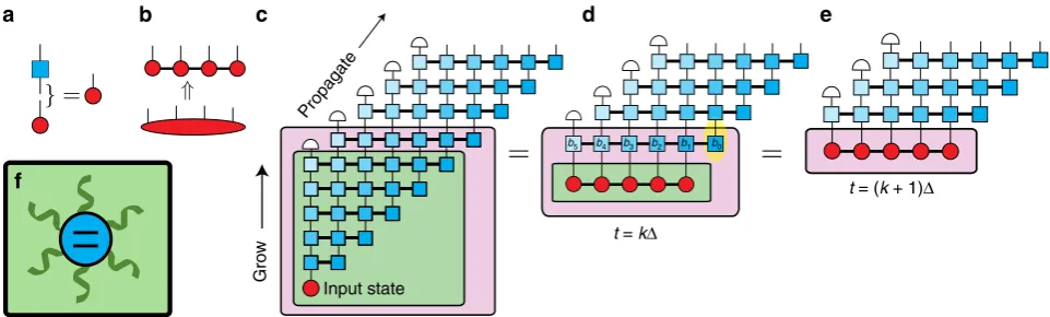
shown in Fig.1a. The red circle represents the density operator, with the protruding‘leg’indicating this is a tensor of rank one, that is, a vector. This leg is indexed by an integeri=1,…,d2. The
blue square with two legs represents the propagator eΔL, written as ad2×d2 superoperator1. The matrix–vector multiplication in Eq. (1) is shown by joining a leg of the propagator to the density operator, indicating tensor contraction. This contraction gen-erates the density operator at timet+Δ.
In order to capture non-Markovian dynamics, we extend our representation of the state at time t from a vector to an ADT, representing the history of the system. This is motivated by the path integral of a system interacting linearly with a bosonic environment. After integrating out the environment, the influence of the environment on the system can be captured by an‘influence functional’ of the system paths alone1. The influence functional couples the current evolution to the history, and captures the
non-d
f
a b c e
t = (k + 1)Δ
t = kΔ
b5 b4 b3 b2 b1 b0
Input state
Gro
w
Propagate
Fig. 1Schematic description of the TEMPO algorithm.aPictorial representation of matrix–vector multiplication. Inbwe show how the ADT can be
decomposed into an MPS.cThe full tensor network starting from an initial standard density operator which is grown to an ADT withKlegs, as shown in
d, where we have contracted the contents of the green box. To propagate forward one step, we contract the ADT with the next row of the propagator, as in
[image:2.595.57.538.546.691.2]Markovian dynamics. Makri and Makarov28,29 showed that by considering discrete timesteps, and writing the sum over system states in a discrete basis, the path integral could be reformulated as a propagator for the ADT, written as a discretesum over paths. The influence functional becomes a series of influence functions Ik(j,j′) that connect the evolution of the amplitude of statejto the amplitudes of statesj′an integer number,k, of timesteps ago. This approach is known as the quasi-adiabatic path integral (QUAPI). As described so far, the ADT grows at each timestep, to record the lengthening system history. However, the influence functions have no effect oncekΔexceeds the bath correlation timeτc. One
can therefore propagate an ADT containing only the previous K=τc/Δ steps: this is the finite memory approximation. This
means we consider an ADT of rank K, written as Ai1;i2;¼;iKðtÞ,
where each index runs overik=1,…,d2. The explicit construction of this tensor is described in the Methods section. In general Ai1;i2;¼;iKðtÞ contains d2K numbers, which scales exponentially
with the correlation timeτc. If the full tensor is kept, one quickly
encounters memory problems, and typical simulations are restricted toK< 2031,32. Improved QUAPI algorithms33,34show that (for some models) typical evolution does not explore this entire space, leading us to seek a minimal representation of the ADT.
Matrix product states (MPS)35,36are natural tools to represent high-rank tensors efficiently where correlations are constrained in some way. Examples include the ground state of one-dimensional (1D) quantum systems with local interactions37, steady state transport in 1D classical systems38or time-evolving 1D quantum
states39. Inspired by these results, we show how an ADT can be
efficiently represented and propagated using standard MPS methods. One may decompose high-rank tensors into products of low-rank tensors using SVDs and truncation. By combining indices, the tensorAcan be written as36:
Afi1;¼;ikg;fikþ1;¼;iKg¼Ufi1;¼;ikg;αλα Vy α;i
kþ1;¼;iK
f g: ð2Þ
Here,U,Vare unitary matrices, andλαdenotes a singular value of
the matrixA. Truncation corresponds to throwing away singular valuesλαsmaller than some cutoffλc, consequently reducing the
size of the matrices U, V. This procedure can be iterated by sweepingkacross the whole tensor. The result of this is shown graphically in Fig.1b, and can be written as:
Ai1;¼;ik;¼;iK ¼ai1 α1a
i2 α1;α2¼a
ik
αk1;αk¼a
iK
αK1: ð3Þ
This provides an efficient representation of the state, with a precision controlled by λc.
Ai1;i2;¼;iKðtÞ can be time locally propagated using a tensor
Bji;¼;jK
i1;¼;iK. Crucially, this propagation can be performed directly on
the matrix product representation of A. Moreover, the tensor product description of Bji;¼;jK
i1;¼;iK, shown as the connected blue
squares in Fig.1c, has a small dimension,d2, for the internal legs.
Similarly to the time evolution shown in Fig.1a, the stateA(t+
Δ) is generated by contracting the legs ofA(t) with the input legs of B. Contracting a tensor network with a MPS, and truncating the resulting object by SVDs is a standard operation36. In all the applications we discuss below, wefind that as time propagates we are able to maintain an efficient representation of Ai1;i2;¼;iKðtÞ
with precision determined byλc.
The structure of the propagator depends on the influence functionsIk(j,j′) as shown in Fig.1c (see also Methods section). We use darker colours to represent influence functions corresponding to more recent time points, which are expected to generate stronger correlations in the ADT. The input and output legs of the propagator are offset in thefigure, so time can be viewed as propagating from left to right. In effect, at each step
the register is shifted so that the right-most output index corresponds to the new state: events that occurred more thanτc
ago are dropped, as illustrated by the white semicircles in Fig.1, since they do not influence the future evolution. Evolution over a series of timesteps is depicted in Fig.1c–e. In Fig.1c we show the full tensor network. Assuming the initial state of the system is uncorrelated with its environment means it can be drawn as a regular density operator. In the ‘grow’ phase, a series of asymmetricB propagators are applied, which allow the relevant system correlations to extend in time. Once the system has grown to an object withKlegs, we enter the regular propagation phase, shown in Fig.1d, e.
Spin-boson phase transition. To demonstrate the utility of the TEMPO algorithm, we apply it to two problems of a quantum system coupled to a non-Markovian environment. Wefirst con-sider the unbiased SBM30, which has long served as the proving
ground for open system methods. The generic Hamiltonian of this model is
H¼ΩSxþ X
i
Sz giaiþgia
y
i
þωiayiai; ð4Þ
where the Si are the usual spin operators, ayi(ai) and ωi are, respectively, the creation (annihilation) operators and frequencies of theith bath mode, which couples to the system with strength gi. The behaviour of the bath is characterised by the spectral density function
JðωÞ ¼X i
gi
j j2δ ωω
i
ð Þ: ð5Þ
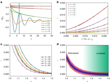
This model is known to show a rich variety of physics depending on the particular form of spectral density and system parameters chosen. When the spectral density is Ohmic, JðωÞ ¼2αωexpðω=ωcÞ, the model is known to exhibit a quantum phase transition in the BKT universality class40, at a critical value of the system–environment coupling α=αc30,41.
The transition takes the system from a delocalised phase belowαc,
where any spin excitation decays (〈Sz〉=0 in the steady state), to a localised phase above αc (〈Sz〉≠0 in the steady state). Most
analytic results are restricted to the regime where the cutoff frequency ωcΩ. For example, when S describes a spin-1/2
particle, the phase transition occurs atαc¼1þ OðΩ=ωcÞ30,40,42.
We are able to explore the dynamics around this phase transition using TEMPO. In Fig. 2a we show the polarisation dynamics of the spin-1/2 SBM for a range ofαatK=200. This memory length is an order of magnitude larger than standard ADT implementations30and is required to reach the asymptotic limit of the dynamics in the vicinity of the phase transition. We achieve convergence by varying the timestepΔand SVD cutoffλc.
We take an initial condition 〈Sz〉= +1/2 with no excitations in the environment, andfind〈Sz(t)〉.
Before reaching the localisation transition atα=αc, onefirst
the memory cutoff τc→KΔ. We should thus examine how the
extracted decay rate,γ, depends on the memory cutoff. Forα<αc,
γshould remainfinite asτc→∞, while forα>αcit should vanish.
In Fig.2b we plotγas a function of 1/K=Δ/τcfor different values
of αaround the phase transition. At small α, γdoes appear to remain finite as K→∞, while at large α the behaviour appears consistent with localisation.
We may estimate the location of the phase transition by extrapolating 1/K→0 for eachα, andfinding the smallest value of
αconsistent with γ→0. To do this, we use cubicfits in Fig. 2b (solid lines), and extract the constant part, with the restriction that the extractedγcannot be negative. In order tofind the phase transition as accurately as possible, we must perform simulations up to very large values ofK: we here perform simulations up to K=200, something that would be simply impossible without the tensor compression we exploit. Errors in ourfits are assessed by monitoring the sensitivity of the best-fit result to truncation precisionλc. These errors are all <10−4 and so are smaller than
the points in Fig.2. This allows us tofind an error in the extracted K→∞limit. The extracted values for γare displayed in Fig.2d where we show our estimate for its 68 and 95% confidence intervals. These suggest thatαc’1:25, consistent with the known analytic results30,40,42. We note that identifyingαcprecisely from
the time dependence of〈Sz〉is particularly challenging: since the localisation transition is in the BKT class40, the order parameter
approaches zero continuously.
The efficiency of TEMPO enables consideration of models with a larger local Hilbert space. To demonstrate this, we examine the localisation transition in the spin-1 SBM. Physically this could either arise from a spin-1 impurity or from a pair of spin-1/2 particles interacting with a common environment44. On
switch-ing to this problem, the local dimension of each leg of our state
tensor increases fromd2=4 tod2=9, reducing the values ofK
we can reach. However, we also find convergence occurs for larger timesteps, allowing access to similar values ofτc.
In Fig.3a we show the dynamics of this model, after initialising to〈Sz〉=1. In this case, on both sides of the localisation transition, the dynamics shows complex oscillatory behaviour before settling down to an exponential decay. This introduces more uncertainty to our exponentialfits. However, as shown in Fig.3b the extracted decay rate vanishes atαc’0:28, indicative of the phase transition and agreeing with numerical renormalisation group results44,45, but in contrast to the results found using a variational ansatz46.
Two spins in a common environment. We next demonstrate the
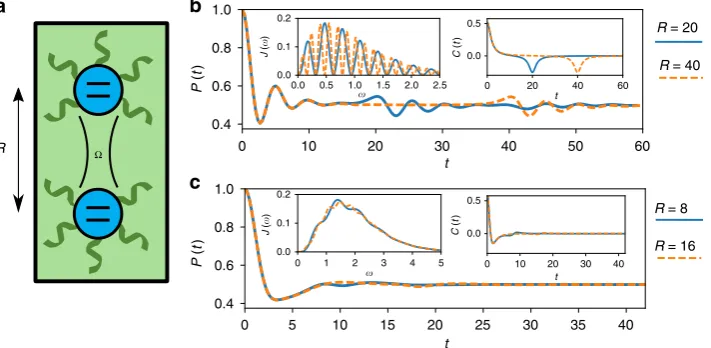
flexibility of TEMPO by applying it to a dynamical problem for which other methods are not available. We consider a pair of identical spins-1/2, at positionsraandrb, which couple directly to each other through an isotropic Heisenberg coupling Ω, and which both couple to a common environment, see Fig. 4a. The Hamiltonian reads:
H ¼ΩSaSbþX ν¼a;b
X
i
Sz;ν gi;νaiþgi;νayi
þωia
y
iai: ð6Þ
The system–bath coupling constants have a position-dependent phase, gi;ν¼gieikirν, where ki is the wavevector of the ith bosonic mode. We assume linear dispersionωi=c|ki| andc=1. This model exhibits complex dissipative dynamics on two different timescales. The faster timescale describes dissipative dynamics of the spins due to interactions with their nearby environment, typically set by the ωc defined earlier. The other
timescale is set by the spin separation R=|ra−rb| over which there is an environment-mediated spin–spin interaction. By
0.000 0.005 0.010 0.015 0.020
1 / K = Δ / C
0.000 0.005 0.010 0.015 0.020 0.025
= 1.0 = 1.1 = 1.2 = 1.3 = 1.4 = 1.5
b a
1.0 1.1 1.2 1.3 1.4 1.5
0.000 0.001 0.002 0.003 0.004
d
0
〈
Sz
〉
5 10 15
t
20 25 30
–0.2 0.0 0.2 0.4
1.0 1.1 1.2 1.3 1.4 1.5
0.000 0.001 0.002 0.003 0.004
K = 100 K = 120 K = 140 K = 150 K = 200
c
a
Localised Delocalised
= 0.1
= 0.3 = 0.7 = 1.0 = 1.2 = 1.5
[image:4.595.110.487.49.331.2]changing R we can control the ratio of these timescales. The dimension, D, of the bath also has an effect: the intensity of environmental excitations propagating from one spin to the other will be stronger for lowerD.
When the spins are close together, R<ω1
c , it is difficult to
distinguish local dissipative effects from the environment-mediated interaction and both master equation techniques13
and the standard ADT method47 generate accurate dynamics. Instead, we consider large separationR>ω1
c , about which little is
known. The ADT then requires both a small timestepΔω1 c
to capture the fast local dissipative dynamics and a large cutoff time τc=KΔ>R to capture environment-induced interactions;
hence, a very large K is needed. Using TEMPO we are able to investigate these dynamics without even having to go beyond the tensor growth stage shown in Fig. 1c, and thus avoid any error caused by afinite memory cutoffK.
We project onto the Sz,a+Sz,b=0 subspace of the system, consisting of the two anti-aligned spin states, since this is the only sector with non-trivial dynamics. The effective Hamiltonian for this 2dsubspace can then be mapped onto the spin-1/2 SBM, Eq. (4), albeit with a modified spectral density that depends on R. Details of this procedure are given in the Methods section.
In Fig. 4b, c we show dynamics for different R for environments with D=1 and D=3. Insets show the effective spectral densities,J(ω), and real part of the bath autocorrelation functions, C(t), which we define in the Methods section. We initialise the spins in a product state with 〈Sz,a〉=1/2, 〈Sz,b〉= −1/2 and calculate the probability,P(t), offinding the system in this state at timet. The bath is initialised in thermal equilibrium at temperature T. ForD=1, after initial oscillations decay away over a timescaleω1
c , there are revivals att=R. This is due to
the strongly oscillating spectral density which results in a large peak at C(t=R). As expected for a one-dimensional environ-ment, the profile of these secondary oscillations is independent of RwhenRω1
c . Additionally forR=20 more small amplitude
oscillations appear att≈40, due to the effective interaction of the spins at t≈20 sending more propagating excitations into the environment. For D=3 the spectral density still has an oscillatory component, though it is much less prominent. The resulting peaks atC(t=R) are thus much smaller than thet=0 peak and have only a small effect on the dynamics. Small amplitude oscillations can be seen att≈RwhenR=8, but with R=16 it is difficult to see any significant features in the dynamics.
0 20 40 60 0.0
0.5
0 10 20 30 40 50 60
0.4 0.6 0.8 1.0
0 5 10 15 20 25 30 35 40
0.4
t t
t
t
J
(
)
J
(
)
R
R = 20
R = 40
R = 8
R = 16
P
(
t
) C
(
t
)
P
(
t
)
0.6 0.8 1.0
a
0.0 0.5 1.0 1.5 2.0 2.5 0.0
0.1 0.2 b
c
0 10 20 30 40 0.0
0.5
0 1 2 3 4 5 0.0
0.1 0.2 Ω
C
(
t
)
Fig. 4Dynamics of two coupled spins-1/2, separated by a distanceR, interacting with the same environment.aA schematic of this system.b,cDynamics of the system in 1D and 3D, respectively, at different values of the spin separationR. Insets to these plots are the corresponding spectral densities and bath correlation functions (see Methods section for details). The dimensionless couplingsαused for 1D and 3D areα=2 andα=1, respectively. We set the speed of soundc=1, so that all parameters are in units ofΩand we chooseT=0.5,ωc=0.5. In all cases we have used 180 timesteps, but not used the
memory cutoff meaningK=180
0 5 10 15 20
t
25 30
0.0 0.2 0.4 0.6 0.8 1.0
= 0.15 = 0.2 = 0.25 = 0.3 = 0.35 = 0.4
0.15 0.20 0.25 0.30 0.35 0.40
0.000 0.025 0.050 0.075 0.100 0.125 0.150
Localised Delocalised
K = 50 K = 60 K = 70 K = 80
a b
〈
Sz
〉
[image:5.595.124.479.52.183.2] [image:5.595.122.478.237.411.2]
Discussion
We have presented a highly efficient method for modelling the non-Markovian dynamics of open quantum systems. Our method is applicable to a wide variety of situations. In well-established ADT methods, non-Markovianity is accounted for by encoding the system’s history in a high-rank tensor; we have overcome the restrictive memory requirements of storing this tensor by repre-senting it as an MPS. We can then efficiently calculate open system dynamics by propagating this MPS via iterative applica-tion of an MPO. To test our technique we used it to find the localisation transition in the SBM, for both spin-1/2 and spin-1, and found estimates for the critical couplings, consistent with other techniques. We then applied our method to a pair of interacting spins embedded within a common environment, in a regime where a large separation of timescales prevents the use of other methods.
Precisely locating the phase transition is a rigorous test of any numerical method: as we found, very large memory times, up to K=200 were required to precisely locate this point. Other improved numerical methods22,23,33have demonstrated a degree of enhanced efficiency when considering conditions away from the critical coupling. As yet, other such general methods have not been used to precisely locate the transition.
The key to our technique is that tensor networks provide an efficient representation of high-dimensional tensors encoding restricted correlations. As well as the widespread application of such methods in low-dimensional quantum systems35–39, they have also been applied to sampling problems in classical statistical physics48, and analogous techniques (under the name ‘Tensor
trains’) have been developed in computer science49. Moreover, there has been a recent synthesis showing how techniques developed in one context can be extended to others, such as machine learning50, or Monte Carlo sampling of quantum states51. Our work defines a further application for these meth-ods, and future work may yet yield even more efficient approaches.
The methods described in this article are already very powerful in their ability to model general non-Markovian environments. They also enable easy extension to study larger quantum systems, by adapting other methods from tensor networks such as the optimal boson basis52—these will be the subject of future work.
They may also be combined with approaches such as the tensor transfer method described in Ref. 53. This method allows efficient long time propagation of dynamics, so long as an exact map is known up to the bath memory time: TEMPO enables efficient calculation of the required exact map. With such tools available, the study of the dynamics of quantum systems in non-Markovian environments3can now move from studying isolated examples to
elucidating general physical principles, and modelling real systems.
Methods
TEMPO algorithm. In this section, we will present the details of the TEMPO algorithm, paying particular attention to how the ADT and propagator are con-structed in a matrix product form.
The generic Hamiltonian of the models we consider is
H¼H0þO
X
i
giaiþgia
y
i
þX
i
ωia
y
iai; ð7Þ
¼H0þHE; ð8Þ
whereH0is the (arbitrary) free system Hamiltonian andHEcontains both the bath
Hamiltonian and the system–bath interaction. Hereayi(ai) andωiare the creation
(annihilation) operators and frequencies of theith environment mode. The system
operatorOcouples to bath modeiwith coupling constantgi. As outlined in the
main text, we work in a representation whered×ddensity operators are given
instead by vectors withd2elements. These vectors are then propagated using a
Liouvillian as in Eq. (1) of the main text,L ¼ L0þ LE, whereL0andLEgenerate
coherent evolution caused byH0andHE, respectively. It has been shown recently
that it is straightforward to include additional Markovian dynamics in the reduced system Liouvillian54in the ADT description.
If the total propagation over timetNis composed ofNshort time propagators etNL¼ ðeΔLÞN, we can use a Trotter splitting55
eΔLeΔLEeΔL0þ OðΔ2Þ: ð9Þ
We note that the following arguments can be easily adapted to use the higher-order, symmetrized, Trotter splitting28,29,56that reduces the error toΔ3. All the
numerical results presented use this symmetrized splitting, but for ease of exposition we use the form of Eq. (9) here. We assume the initial density operator factorises into system and environment terms, with the environment initially in thermal equilibrium at temperatureT. Time evolution can then be written as a path sum over system states, by inserting resolutions of identity between each eΔLEeΔL0
and then tracing over environmental degrees of freedom. The result is the discretized Feynman–Vernon influence functional28,29, which yields the following
form for the time evolved density matrix:
ρjNðtNÞ ¼
X
j1;¼;jN1
YN
n¼1
Y
n1
k¼0
Ikðjn;jnkÞ
!
ρj1ðΔÞ: ð10Þ
The indexing here is in a basis whereOis diagonal. Eachjindex runs from 1 tod2,
and due to the order of the splitting in Eq. (9), the initial state of the system has been propagated forward a single timestep,ρj1ðΔÞ ¼ e
ΔL0
j1j0ρj0ð0Þ. We have
defined the influence functions
Ikðj;j′Þ ¼ eϕk
ðj;j′Þ; k≠1;
eΔL0
jj′eϕ1ðj;j′Þ; k¼1;
(
ð11Þ
with
ϕkðj;j′Þ ¼ O
jðOj′Re½ηk þiO
þ
j′Im½ηk Þ: ð12Þ
HereOj are thed2possible differences that can be taken between two eigenvalues
ofOandOþj the corresponding sums. The coefficients,ηk, quantify the
non-Markovian correlations in the reduced system acrossktimesteps of evolution and
are given by the integrals
ηnn′¼
Rtn
tn1dt′
Rtn′
tn′1dt′′Cðt′t′′Þ; n≠n′;
Rtn
tn1dt′
Rt′
tn1dt′′Cðt′t′′Þ; n¼n′;
8 <
: ð13Þ
whereC(t) is the bath autocorrelation function
CðtÞ ¼Z1
0
dωJðωÞcoth ω
2T cosðωtÞ isinðωtÞ
h i
; ð14Þ
with temperature measured in units of frequency and with the spectral density JðωÞ ¼Pijgij2δðωiωÞ.
The summand of the discretised path integral in Eq. (10) can be interpreted as the components of anN-index tensorAjN;jN1;¼;j1. This tensor is an ADT of the
type originally proposed by Makri and Makarov28,29. We will show below that this
N-index tensor can also be written as tensor network consisting ofN(N+1)/2 tensors with, at most, four legs each and that this network can be contracted using standard MPS-MPO contraction algorithms35,36, First we gather terms in the inner
piece of the double product in Eq. (10) into a single object, which we write as
components of ann-index tensor
Bjn;jn1;¼;j1¼Y
n1
k¼0
Ikðjn;jnkÞ: ð15Þ
Next, we define the (2n−1)-index tensors
Bjn;jn1;¼;j1
in1;¼;i1 ¼
Y
n1
k¼1 δjnk
ink
!
Bjn;jn1;¼;j1; ð16Þ
forn> 1, and the 1-index initial ADT:
Aj1¼ Bj1ρj1ðΔÞ: ð17Þ
We may now evolve this ADT in time iteratively by successive contraction of tensors. This process is shown graphically in Fig.1c. Thefirst contraction produces a 2-index ADT which describes the full state and history at the second time point:
Aj2;j1¼Bj2;j1
i1 A
We next contract withBj3;j2;j1
i2;i1 to produce a 3-index ADT and so on. Thenth step of
this process then looks like
Ajn;jn1;¼;j1¼Bjn;jn1;¼;j1
in1;¼;i1 A
in1;in2;¼;i1; ð19Þ
and the density operator for the open system at timetn=nΔis recovered by summing over all but thejnleg,
ρjnðt
nÞ ¼
X
jn1;¼;j1
Ajn;jn1;¼;j1;
ð20Þ
from which observables can be calculated. At each iteration the size of the ADT grows by one index, since up to now we have made no cutoff for the bath memory time: we are in the‘grow’phase depicted in Fig.1c. To compress the state after each application of thisBtensor, we sweep along the resulting ADT performing SVD’s and truncating at each bond, throwing away the components corresponding to singular values smaller than our cutoffλc. This gives an MPS representation of the
ADT, as given in Eq. (3). As discussed in Ref.57, we must in fact sweep both left to
right and then right to left to ensure the most efficient MPS representation is found. If no bath memory cutoff is made, this whole process is repeated until the
final time point is reached atn=N.
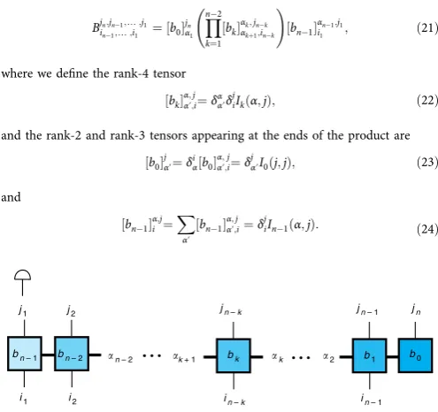
The (2n−1)-index propagation tensor,B, can be represented as an MPO such
that the above process of iteratively contracting tensors becomes amenable to standard MPS compression algorithms35,36. The form required is
Bjn;jn1;¼;j1
in1;¼;i1 ¼ ½b0
jn α1
Y
n2
k¼1
½bkαk;jnk αkþ1;ink
!
bn1
½ αn1;j1
i1 ; ð21Þ
where we define the rank-4 tensor
bk ½ α;j
α′;i¼δαα′δjiIkðα;jÞ; ð22Þ
and the rank-2 and rank-3 tensors appearing at the ends of the product are
b0
½ j
α′¼δiα½ b0α;α′;ji¼δ j
α′I0ð Þj;j; ð23Þ
and
bn1
½ α;j
i ¼
X
α′
½bn1 α;j
α′;i¼δ j
iIn1ðα;jÞ: ð24Þ
Upon substituting these forms, Eqs. (22)–(24), into Eq. (21) it is straightforward to verify that we recover the expression Eq. (16). The rank-(2n−1) MPO, Bjn;jn1;¼;j1
in1;¼;i1 , is represented by the tensor network diagram in Fig.5.
We note it has recently been shown that if the spectrum ofOhas degeneracies, then part of the sum in Eq. (10) can be performed analytically, vastly reducing computational cost of the ADT method for systems where the environment only couples to a small subsystem58. Here we can further exploit the fact that, even when
there is no degeneracy in thedeigenvalues ofO, there is always degeneracy in the d2differences between its eigenvalues,O
j, that is,dof these differences are always
zero. Using the same partial summing technique described in Ref.57we can thus
reduce the dimension of the internal indices of the rank-(2n−1) MPO, Eq. (21), fromd2tod2−d+1. Furthermore, if the eigenvalues ofOare non-degenerate but
evenly spaced, as is the case for spin operators, then there are only 2d−1 unique values ofOj, allowing us to reduce the size of thebktensors, Eq. (22), fromOðd8Þ toOðd6Þ.
Thefinite memory approximation can now be introduced by throwing away
information in the ADT for times longer thanτc=KΔinto the system’s history. To
do this we write
½bkα;j
α′;i¼δαα′δji k>K: ð25Þ
Thus, when propagatingAjn;¼;j1beyond theKth timestep only indicesjntojn −K+1
have any relevance and we can sum over the rest. The way we do this in practice is
to define the 2K-leg tensor MPO
BjKþ1¼;j2
iK;¼;i1 ¼
X
j1
BjKþ1;jK;¼;j1
iK;¼;i1 ; ð26Þ
such that contraction with a rank-KMPS is equivalent tofirst growing the MPS by one leg and then summing over (i.e. removing) the leg which is earliest in time.
Repeating this contraction propagates anA-tensor MPS forward in time, but
maintains its rank ofKfor all timestepsn>K. This is what we show in the
‘propagate’phase of Fig.1c. For some spectral densities, it is possible to improve the convergence withτcby making a softer cutoff59,60, but since TEMPO can go to
very large values ofKthis is not necessary here.
For time-independent problems (as we study here), the‘propagate’phase involves repeated contraction with the same MPO, Eq. (26), which is independent of the timestep. To make this clear, it is convenient to change our index labelling (which, so far has referred to the absolute number of timesteps fromt=0). We will instead relabel the indices on the MPO and MPS as follows:BjKþ1;¼;j2
iK;¼;i1 !B
j1;¼;jK
i1;¼;iK
andAjn;¼;jnKþ1!Aj1;¼;jKðt
nÞ. The indices now refer to the distance back in time from the current time point. To summarise, with the new labelling wefirst grow the initial state into aK-index MPS,Aj1;¼;jKðτ
cÞ, and then propagate as:
Aj1;¼;jKðtþΔÞ ¼Bj1;¼;jK
i1;¼;iKA
i1;¼;iKðtÞ; ð27Þ
and the physical density operator is found via
ρj1ðtÞ ¼ X
j2;¼;jK
Aj1;¼;jKðtÞ:
ð28Þ
Having described the TEMPO algorithm we now briefly analyse the
computational cost of applying it to the SBM of Eq. (4). In Fig.6a we plot the total size,Ntot, of the MPS and maximum bond dimension,λmax, used to obtain
converged results in Fig.2against coupling strength withK=200. Wefind the
most computationally demanding regime to be aroundα=0.5, the point of
crossover from underdamped to overdamped oscillations ofSz. Wefind the CPU
time required is linear in the total memory requirement. For the largest memory
required (atα=0.5), the time to obtain 500 data points using TEMPO on the HPC
Cirrus cluster was≈20.5 h. In Fig.2b we show howNtotgrows withKfor different
values ofα. Forα=0.1,0.5 we see quadratic growth withK, while for couplings near and above the phase transition,α=1,1.5, the growth is only linear. Both cases
j2
j1
i1 i2
bn – 1 bn – 2 n – 2 k + 1 k 2
in – k in – 1
jn – k jn – 1 jn
bk b1 b0
Fig. 5Tensor network diagram depicting the MPO decomposition of the
rank-(2n+1) tensor,B. The squares show thebktensors in Eqs. (22)–(24),
withkincreasing right to left. Theinandjntensor indices correspond to the
vertical legs withnincreasing from left to right. Whenn=Kthej1leg is summed over to give the rank-2Kpropagation phase MPO, represented in thefigure by contraction with a rank-1 object; thed2-dimensional vector whose elements are all equal to one
0.0 0.2 0.4 0.6
Ntot
K Ntot
/1
0
7
Ntot
/1
0
7
0.8 1.0
1.0
1.2 1.4 0
50 100 max
max
150 200 250
a
50 75 100 125 150 175 200
0.0 0.5 1.5 2.0 2.5 3.0 3.5
1.0
0.0 0.5 1.5 2.0 2.5 3.0
3.5 b
= 1.5 = 1 = 0.5 = 0.1
Fig. 6Memory requirements of the TEMPO algorithm. We show both the total size of thefinal MPS,Ntot, and the maximum bond dimension,λmax, as a
[image:7.595.43.291.254.487.2] [image:7.595.119.479.600.710.2]thus represent polynomial scaling, a substantial improvement on the exponential scaling of the standard ADT method for which one hasNtot=4K.
Mapping two spins in a common environment to a single spin model. We show here how to map Eq. (6) describing a pair of spin-1/2 particles in a common environment onto Eq. (4), a single spin-1/2 SBM. The Hamiltonian Eq. (6)
has the property that the totalz-component of the two-spin system is conserved,
[Sz,a+Sz,b,H]=0. Thus, the problem can be separated into three distinct sub-spaces: the two states with the spins anti-aligned (Sz,a+Sz,b=0) form one subspace and the two aligned spin states (Sz,a+Sz,b=±1) are the other two. The one-dimensional subspaces with aligned spins cannot evolve in time; hence, all non-trivial dynamics in this model happen in theSz,a+Sz,b=0 subspace. We therefore focus on this subspace. By doing so, we may subtract a term proportional toSz,a+ Sz,bfrom the system–bath coupling in Eq. (6). The remaining system–bath inter-action is given by
1
2 Sz;aSz;b
X
i
~
gi j jaiþj ja~gi y
i
: ð29Þ
The effective coupling here isj j ¼~gi gi;agi;b¼2gisin½ki ðrarbÞ=2 . These couplings lead to a modified effective spectral density13,61,
Jð Þ ¼ω 2Jpð Þωð1FDðωRÞÞ; ð30Þ
whereJp(ω) is the actual density of states of the bath. The functionFD(ωR) arises
from angular averaging inD-dimensional space, and so crucially depends on the
dimensionality of the environment. Specifically we have:
FDðxÞ ¼
cosðxÞ; D¼1;
J0ðxÞ; D¼2;
sincðxÞ; D¼3;
8 > < >
: ð31Þ
whereJ0(x) is a Bessel function. We note thatFD(ωR)→0 asR→∞forD> 1, due to the diminishing effect of the environment-induced coupling in higher dimensions.
(When consideringR→∞, we should note that in the original Hamiltonian we
neglected any retardation in the Heisenberg interaction.) At small separations,R→ 0,FD(ωR)→1 and soJ(ω)→0 for allDdue to the loss of relative phase shift between the couplings of the anti-aligned states to the environment.
For the bare density of statesJp(ω), we consider a simple model of e.g. a quantum dot in a phonon environment, for which the coupling constants appearing in the Hamiltonian, Eq. (6), havegi ffiffiffiffiffiωi
p 19
. This means that in the
continuum limit the spectral density for aD-dimensional environment is
JpðωÞ ¼
α
2
ωD
ωD1 c
eω=ωc; ð32Þ
whereωcdescribes a high-frequency cutoff andαis the strength of the interaction
with the environment.
Data and code availability. The datasets generated during and/or analysed during the current study are available at:
https://doi.org/10.17630/44616048-eaac-4971-bbff-1d36e2cef256. The TEMPO code is available athttps://doi.org/10.5281/
zenodo.1322407.
Received: 5 May 2018 Accepted: 11 July 2018
References
1. Breuer, H. -P. & Petruccione, F.The Theory of Open Quantum Systems
(Oxford University Press, Oxford, 2002).
2. Walls, D. F. & Milburn, G. J.Quantum Optics2nd edn (Springer, Berlin, 2007).
3. de Vega, I. & Alonso, D. Dynamics of non-Markovian open quantum systems.
Rev. Mod. Phys.89, 015001 (2017).
4. Gröblacher, S. et al. Observation of non-Markovian micromechanical
brownian motion.Nat. Commun.6, 7606 (2015).
5. Madsen, K. H. et al. Observation of non-Markovian dynamics of a single
quantum dot in a micropillar cavity.Phys. Rev. Lett.106, 233601 (2011). 6. Mi, X., Cady, J. V., Zajac, D. M., Deelman, P. W. & Petta, J. R. Strong coupling
of a single electron in silicon to a microwave photon.Science355, 156–158 (2017).
7. Potočnik, A. et al. Studying light-harvesting models with superconducting circuits.Nat. Commun.9, 904 (2018).
8. Aharonovich, I., Englund, D. & Toth, M. Solid-state single-photon emitters. Nat. Photon.10, 631–641 (2016).
9. Chin, A. W. et al. The role of non-equilibrium vibrational structures in
electronic coherence and recoherence in pigment–protein complexes.Nat.
Phys.9, 113–118 (2013).
10. Lee, M. K., Huo, P. & Coker, D. F. Semiclassical path integral dynamics: photosynthetic energy transfer with realistic environment interactions.Annu. Rev. Phys. Chem.67, 639–668 (2016).
11. Barford, W.Electronic and Optical Properties of Conjugated Polymers(Oxford
University Press, Oxford, 2013).
12. McCutcheon, D. P. S., Dattani, N. S., Gauger, E. M., Lovett, B. W. & Nazir, A. A general approach to quantum dynamics using a variational master equation:
application to phonon-damped rabi rotations in quantum dots.Phys. Rev. B
84, 081305 (2011).
13. McCutcheon, D. P. S. & Nazir, A. Coherent and incoherent dynamics in excitonic energy transfer: correlatedfluctuations and off-resonance effects. Phys. Rev. B83, 165101 (2011).
14. Kaer, P., Nielsen, T. R., Lodahl, P., Jauho, A.-P. & Mørk, J. Non-Markovian model of photon-assisted dephasing by electron–phonon interactions in a coupled quantum-dot–cavity system.Phys. Rev. Lett.104, 157401 (2010). 15. Roy, C. & Hughes, S. Influence of electron–acoustic-phonon scattering on
intensity power broadening in a coherently driven quantum-dot–cavity
system.Phys. Rev. X1, 021009 (2011).
16. Segal, D. & Agarwalla, B. K. Vibrational heat transport in molecular junctions. Annu. Rev. Phys. Chem.67, 185–209 (2016).
17. Subotnik, J. E. et al. Understanding the surface hopping view of electronic transitions and decoherence.Annu. Rev. Phys. Chem.67, 387–417 (2016). 18. Bylicka, B., Chruściński, D. & Maniscalco, S. Non-Markovianity and reservoir
memory of quantum channels: a quantum information theory perspective.Sci.
Rep.4, 5720 (2014).
19. Xiang, G.-Y. et al. Entanglement distribution in opticalfibers assisted by nonlocal memory effects.Phys. Lett.107, 54006 (2014).
20. Mahan, G. D.Many Particle Physics3rd edn (Springer, Berlin, 2000).
21. Jang, S. Theory of coherent resonance energy transfer for coherent initial condition.J. Chem. Phys.131, 164101 (2009).
22. Cohen, G., Gull, E., Reichman, D. R. & Millis, A. J. Taming the dynamical sign
problem in real-time evolution of quantum many-body problems.Phys. Rev.
Lett.115, 266802 (2015).
23. Chen, H.-T., Cohen, G. & Reichman, D. R. Inchworm Monte Carlo for exact non-adiabatic dynamics. ii. Benchmarks and comparison with established
methods.J. Chem. Phys.146, 054106 (2017).
24. Yoshitaka, T. & Kubo, R. Time evolution of a quantum system in contact with a nearly Gaussian-Markoffian noise bath.J. Phys. Soc. Jpn.58, 101–114 (1989). 25. Garraway, B. M. Non-perturbative decay of an atomic system in a cavity.Phys.
Rev. A55, 2290–2303 (1997).
26. Iles-Smith, J., Lambert, N. & Nazir, A. Environmental dynamics, correlations, and the emergence of noncanonical equilibrium states in open quantum systems.Phys. Rev. A90, 032114 (2014).
27. Schröder, F. A. Y. N. et al. Multi-dimensional tensor network simulation of open quantum dynamics in singletfission. Preprint athttps://arxiv.org/abs/
1710.01362(2017).
28. Makri, N. & Makarov, D. E. Tensor propagator for iterative quantum time evolution of reduced density matrices. I. Theory.J. Chem. Phys.102, 4600 (1995).
29. Makri, N. & Makarov, D.E. Tensor propagator for iterative quantum time
evolution of reduced density matrices. II. Numerical methodology.J. Chem.
Phys.102, 4611 (1995).
30. Leggett, A. J. et al. Dynamics of the dissipative two-state system.Rev. Mod. Phys.59, 1–85 (1987).
31. Nalbach, P., Ishizaki, A., Fleming, G. R. & Thorwart, M. Iterative path-integral algorithm versus cumulant time-nonlocal master equation approach for dissipative biomolecular exciton transport.N. J. Phys.13, 063040 (2011). 32. Thorwart, M., Eckel, J. & Mucciolo, E. R. Non-Markovian dynamics of double
quantum dot charge qubits due to acoustic phonons.Phys. Rev. B72, 235320
(2005).
33. Sim, E. Quantum dynamics for a system coupled to slow baths: on-the-fly
filtered propagator method.J. Chem. Phys.115, 4450–4456 (2001). 34. Lambert, R. & Makri, N. Memory propagator matrix for long-time dissipative
charge transfer dynamics.Mol. Phys.110, 1967–1975 (2012).
35. Schollwöck, U. The density-matrix renormalization group in the age of matrix product states.Ann. Phys. (NY)326, 96–192 (2011).
36. Orús, R. A practical introduction to tensor networks: matrix product states and projected entangled pair states.Ann. Phys. (NY)349, 117–158 (2014). 37. White, S. R. Density matrix formulation for quantum renormalization groups.
Phys. Rev. Lett.69, 2863–2866 (1992).
38. Derrida, B., Evans, M. R., Hakim, V. & Pasquier, V. Exact solution of a 1d
asymmetric exclusion model using a matrix formulation.J. Phys. A26, 1493
(1993).
40. Florens, S., Venturelli, D. & Narayanan, R. inQuantum Quenching, Annealing and Computation(eds Chandra, A. K., et al.) 145–162 (Springer, Berlin, Heidelberg, 2010).
41. Le Hur, K. inUnderstanding Quantum Phase Transitions(ed. Carr, L.) (CRC
Press, New York, 2010)
42. Bulla, R., Tong, N.-H. & Vojta, M. Numerical renormalization group for
bosonic systems and application to the sub-ohmic spin-boson model.Phys.
Rev. Lett.91, 170601 (2003).
43. Kessler, E. M. et al. Dissipative phase transition in a central spin system.Phys. Rev. A86, 012116 (2012).
44. Orth, P. P., Roosen, D., Hofstetter, W. & Le Hur, K. Dynamics,
synchronization, and quantum phase transitions of two dissipative spins.Phys. Rev. B82, 144423 (2010).
45. Winter, A. & Rieger, H. Quantum phase transition and correlations in the
multi-spin-boson model.Phys. Rev. B90, 224401 (2014).
46. McCutcheon, D. P. S., Nazir, A., Bose, S. & Fisher, A.J. Separation-dependent localization in a two-impurity spin-boson model.Phys. Rev. B81, 235321 (2010).
47. Nalbach, P., Eckel, J. & Thorwart, M. Quantum coherent biomolecular energy transfer with spatially correlatedfluctuations.N. J. Phys.12, 065043 (2010).
48. Johnson, T. H., Elliott, T. J., Clark, S. R. & Jaksch, D. Capturing exponential variance using polynomial resources: applying tensor networks to non-equilibrium stochastic processes.Phys. Rev. Lett.114, 090602 (2015). 49. Oseledets, I. V. Tensor-train decomposition.J. Sci. Comput.33, 2295–2317
(2011).
50. Stoudenmire, E. & Schwab, D. J. inAdvances in Neural Information Processing Systems29(eds. Lee, D. D. et al.) 4799–4807 (Curran Associates, Red Hook, 2016).
51. Ferris, A. J. & Vidal, G. Perfect sampling with unitary tensor networks.Phys. Rev. B85, 165146 (2012).
52. Guo, C., Weichselbaum, A., von Delft, J. & Vojta, M. Critical and strong-coupling phases in one- and two-bath spin-boson models.Phys. Rev. Lett.108, 160401 (2012).
53. Cerrillo, J. & Cao, J. Non-Markovian dynamical maps: numerical processing of open quantum trajectories.Phys. Rev. Lett.112, 110401 (2014). 54. Barth, A. M., Vagov, A. & Axt, V. M. Path-integral description of combined
Hamiltonian and non-Hamiltonian dynamics in quantum dissipative systems. Phys. Rev. B94, 125439 (2016).
55. Trotter, H. F. On the product of semi-groups of operators.Proc. Am. Math.
Soc.10, 545–551 (1959).
56. Suzuki, M. Generalized Trotter’s formula and systematic approximants of
exponential operators and inner derivations with applications to many-body
problems.Comm. Math. Phys.51, 183–190 (1976).
57. Stoudenmire, E. M. & White, S. R. Minimally entangled typical thermal state algorithms.N. J. Phys.12, 055026 (2010).
58. Cygorek, M., Barth, A. M., Ungar, F., Vagov, A. & Axt, V. M. Nonlinear cavity feeding and unconventional photon statistics in solid-state cavity QED revealed by many-level real-time path-integral calculations.Phys. Rev. B96, 201201 (2017).
59. Vagov, A., Croitoru, M. D., Glässl, M., Axt, V. M. & Kuhn, T. Real-time path integrals for quantum dots: quantum dissipative dynamics with superohmic
environment coupling.Phys. Rev. B83, 094303 (2011).
60. Strathearn, A., Lovett, B. W. & Kirton, P. Efficient real-time path integrals for
non-Markovian spin-boson models.N. J. Phys.19, 093009 (2017).
61. Stace, T. M., Doherty, A. C. & Barrett, S. D. Population inversion of a driven two-level system in a structureless bath.Phys. Rev. Lett.95, 106801 (2005).
Acknowledgements
We thank T.M. Stace for useful discussions and J. Iles-Smith for comments on an earlier version of this paper. A.S. acknowledges a studentship from EPSRC (EP/L505079/1). P.K. acknowledges support from EPSRC (EP/M010910/1). D.K. acknowledges support from the EPSRC CM-CDT (EP/L015110/1). J.K. acknowledges support from EPSRC programs 'TOPNES' (EP/I031014/1) and 'Hybrid Polaritonics' (EP/M025330/1). B.W.L. acknowl-edges support from EPSRC (EP/K025562/1). This work used EPCC's Cirrus HPC Service (https://www.epcc.ed.ac.uk/cirrus).
Author contributions
The TEMPO code was developed by A.S., P.K. and D.K., following the identification of the MPS representation by J.K. Analysis of the two applications was performed by A.S., P. K. and B.W.L.. The project was directed by J.K. and B.W.L. All authors contributed to the writing of the manuscript.
Additional information
Competing interests:The authors declare no competing interests.
Reprints and permissioninformation is available online athttp://npg.nature.com/ reprintsandpermissions/
Publisher's note:Springer Nature remains neutral with regard to jurisdictional claims in published maps and institutional affiliations.
Open Access This article is licensed under a Creative Commons Attribution 4.0 International License, which permits use, sharing, adaptation, distribution and reproduction in any medium or format, as long as you give appropriate credit to the original author(s) and the source, provide a link to the Creative Commons license, and indicate if changes were made. The images or other third party material in this article are included in the article’s Creative Commons license, unless indicated otherwise in a credit line to the material. If material is not included in the article’s Creative Commons license and your intended use is not permitted by statutory regulation or exceeds the permitted use, you will need to obtain permission directly from the copyright holder. To view a copy of this license, visithttp://creativecommons.org/ licenses/by/4.0/.