Soft Morphological Filter Optimization Using a
Genetic Algorithm for Noise Elimination
T¨urker Erc¸al Yeditepe University
Department of Computer Engineering Kayıs¸da˘gı 34755, Istanbul , Turkey
Ender ¨Ozcan School of Computer Science
University of Nottingham Nottingham NG8 1BB, UK
Shahriar Asta School of Computer Science
University of Nottingham Nottingham NG8 1BB, UK
Abstract—Digital image quality is of importance in almost all image processing applications. Many different approaches have been proposed for restoring the image quality depending on the nature of the degradation. One of the most common problems that cause such degradation is impulse noise. In general, well known median filters are preferred for eliminating different types of noise. Soft morphological filters are recently introduced and have been in use for many purposes. In this study, we present a Genetic Algorithm (GA) which combines different objectives as a weighted sum under a single evaluation function and generates a soft morphological filter to deal with impulse noise, after a training process with small images. The automatically generated filter performs better than the median filter and achieves comparable results to the best known filters from the literature over a set of benchmark instances that are larger than the training instances. Moreover, although the training process involves only impulse noise added images, the same evolved filter performs better than the median filter for eliminating Gaussian noise as well.
Keywords—Filter Design, Supervised Learning, Genetic Algo-rithm, Image Processing.
I. INTRODUCTION
Noise reduction is an essential concern in image pro-cessing. There are many sources of noise in digital images. For example, transmitting or scanning an image can boost up the noise due to electrical interference from the devices used. There are different types of noises dealt with in image processing such as Gaussian noise, periodic noise or impulsive noise. Many studies have proposed a variety of approaches for the removal of such types of noise. Impulsive noise is often encountered during the image transmission process [21], malfunctioning in camera sensors or faulty memory locations in hardware [3]. There are two common types of impulse noise; salt and pepper and random-valued noise. In this study, impulsive noise elimination problem that requires restoration of the image quality which is reduced by white and black (salt and pepper) spots spread over the images is tackled. There are some previous studies on this topic using different search methods. In most of the previous studies, search methodologies are used as training approaches to optimize filters, then the candidate filters are applied on corrupted images. During the search process the original non-corrupted images are compared to the images produced after filtering. By minimizing the difference between filtered and original images, it is expected that an optimized filter will be obtained.
Initially, well known search methodologies, such as, stan-dard GAs [9] and adaptive immune algorithms [26] were used in the design of standard morphological filters [9] for noise filtering. After soft morphological filters were discovered, soft flat morphological filters were optimized for the same purpose. Approaches, such as simulated annealing and tabu search[7], [6] were employed to this end. Direct mathematical approaches such as median filtering [15] and non-linear filters [22] were also favoured by researchers. Indeed, median filter-ing is regarded as the standard approach to deal with impulsive noise. More sophisticated methods such as Neural Networks combined with fuzzy logic [8], noise removal using B-Splines [10] and use of directional filters [31] were also proposed to tackle the same problem. In this study, a Genetic Algorithm (GA) for optimizing a multi-stage non-flat soft morphological filter is presented. The aim is to eliminate salt and pepper noise on images while preserving the quality as much as possible. Different objectives are combined in a fitness function and an appropriate representation scheme is designed to cover a broad range of filter parameters.
The paper is organized as follows: In the next section (Section II), background information about soft mathematical morphology is given. In Section III, the representation scheme and other relevant components of GA, designed for automati-cally creating a noise elimination filter is explained in detail. In Section IV-A, the experimental settings used to obtain the best filter are explained and performance comparison of the generated filter and median filter is provided over 10 different benchmark images in Section IV. Also, the filters generated for different levels of noise are compared with the latest filters presented in the literature and the improvement of the GA and the fitness function is shown visually and mathematically. Finally, conclusions are provided in Section V.
II. SOFTMATHEMATICALMORPHOLOGY
Mathematical morphology was first introduced as an image processing methodology for binary images [16]. The basic operators used in mathematical morphology are erosion and
dilationoperators that accept the image itself and astructuring element (SE), also referred to as kernel, is input. For more details on mathematical morphology, readers can refer to [24] and [25]. Dilation causes regions of foreground pixels grow in size and holes within those areas shrink, while erosion has a reverse effect.
Later, in gray-scale morphology erosion and dilation opera-tors are replaced withminimumandmaximumoperators as the fundamental morphological operators, respectively. There are also openingandclosingoperators which requires application of dilation and erosion using the same structuring element in a specified order. Up to now, mathematical morphology has been used in many different image processing applications, ranging from noise suppression, feature extraction to object recognition. Soft mathematical morphology was introduced by Koskinen, Astola, and Neuvo [12] in 1991. In this approach, weighted order statistics is used instead of the minimum or maximum. The main difference from the standard morphology is the division of the structuring element into two parts;hard centreandsoft boundary. The numbers in the hard centre part have weights greater than one, which is set by a parameter called rank or repetition parameter. The numbers in the soft boundary part of the SE have weights equal to one.
Given a structural elementB, it is divided into two subsets: the hard centre structural element A and the soft structural elementB\A, where A, B⊆Z2, B\A6=∅, and\ denotes the set difference. Let⊕and⊖representsoft dilationandsoft erosionoperations. Soft dilation and soft erosion of an image
f with rank-orderi are defined as:
⊕B,A,i(f) =maxi{i♦(f(Z−ǫ) +A(ǫ))|ǫ∈FA}
[
{f(Z−δ) +B(δ))|δ∈FB\A} (1)
⊖B,A,i(f) =mini{i♦(f(Z+ǫ)−A(ǫ))|ǫ∈FA}
[
{f(Z+δ)−B(δ))|δ∈FB\A} (2)
where maxi andmini denote theith largest and smallest
value in the set respectively; ♦is the repetition operator and
i♦f(v) = {f(v), f(v), ..., f(v)} (i times); FA and FB\A
represent the field of definition ofAandB\A, respectively. Consequently, soft opening ( Λ) and soft closing (∆ ) of an imagef are defined as:
ΛB,A,i(f) =⊕B,A,i(⊖B,A,i(f)) (3)
∆B,A,i(f) =⊖B,A,i(⊕B,A,i(f)) (4)
It has been shown that soft morphological operations are more robust in noisy conditions and are less sensitive to additive noise and to small variations in object shape [13].
III. GENETICALGORITHMS FORGENERATINGSOFT
MORPHOLOGICALFILTER
Genetic Algorithm (GA) is a well known population-based metaheuristic approach used for solving difficult opti-mization problems [18], [19], [20]. The need to search and try different combinations of operations, structuring elements and parameters expands the search space dramatically and makes the search for the best soft morphological filter well suited for GAs. In this study, GAs are used as a supervised learning mechanism to generate a filter for impulsive noise removal, automatically. Our approach uses GA to optimize the parameters of the soft morphological filter using a set of noisy small training images, then the best found filter is applied to a
set of large test instances corrupted by noise for performance evaluation.
A. Representation
Each candidate solution encoded by a chromosome rep-resents a different filter. In this representation scheme, a soft morphological filter that has up to four stages can be encoded. Each of these four stages can have different morphological operations, parameters and structuring elements.It is shown in a previous study [11] that having multiple stages gives better results compared to a one-staged morphological filter. In the first four genes of the chromosome, the type of the morphological operations for each stage are coded ( 0-No Operator, 1-Erosion, 2-Dilation, 3-Opening, 4-Closing ). By using a No Operator type, the corresponding stage can be eliminated, or by using one of the other operations, the operator can be selected for the corresponding stage.
In the next four genes, the neighbourhood type is encoded. In this study, 4 and 8 neighbourhood types are allowed. In a 4 neighbourhood type, the corners of the SE are not used, but in an 8 neighbourhood type, all the nine elements in the SE are used. First of all, these are the most common ones and some prior tests done showed that, enlarging the search space by allowing all types of SE shapes does not give better results. For this part of the chromosome, zero means a 4-connected type neighbourhood; one means an 8-4-connected type neighbourhood.
The next four genes are also binary like the previous four genes. They encode the information whether the SE is symmetric or not. In a symmetric SE, the numbers are symmetrically placed in all planes (horizontally, vertically and diagonally). However, in a non-symmetric SE, all the numbers can be different. The next 36 genes represent the numbers in the structuring elements of the four stages. 3x3 sized SEs are used in this study; which means each Structuring Element has nine numbers in them. Each slot in an SE has a range of [-255, 255]. In a previous work [11], this range is used and it is shown that [9], [11] expanding the range of the number in the SEs gives better results. A gray scale image has a range of [0, 255]; in order to change a black pixel (255) into a white pixel -255 have to be added, and a value of 255 have to be added for the opposite. Therefore, to cover all the values of a gray scale image, this range is used.
The last two parts are the parameters only used in soft morphology. The next 36 genes represent the hard and soft
elements in the SEs. This part of the chromosome is also binary. Each gene works for a single number in an SE. When encoding, a zero maps to a soft element, and a one maps to a hard element. The last four genes in a chromosome represent
the repetition parameterofthe rank parameterfor each stage. An allele for each gene in this part is in{1, ...,9}. An allele value of 1 in this field indicates a standard morphological filter, while another value changes the operation according to the rules defined in soft mathematical morphology. The values above eight give the same results, as the SEs used in this study have nine numbers in them.
B. Evaluation Function
fitness calculation (evaluation) gives us a value that represents the difference between the filtered noisy image and the original non-noisy image. Therefore, the lower the difference, the better the filter will be. There are different measures in the literature. In this study, we combine four measures (functions/criteria). Mean Absolute Error (MAE) (Eq.5) and Mean Squared Error (MSE) (Eq.6), are two commonly used criteria in the literature. MSE strengthens the influence of differences on the result, however none of those functions has precedence over the other. Shape Error (Eq.7) is a relatively new measure as compared to MAE and MSE. In contrast to the other functions, this criteria takes the whole image into account, which is useful for reconstruction [14].
Those three measures presented so far, are good in smooth-ing the noise and preservsmooth-ing the shape details. Nonetheless, the non-flat structuring elements used in our method tend to change the average pixel value of the image, leading to a different brightness in the resulting image when compared to the original image. In order to overcome this difficulty, the brightness error measure (Eq.8), a method mostly ignored in the literature, is additionally used to bias the search to a direction where the brightness of the resulting image will be close to the original image’s brightness value.
f1= 1
M×N
M X i=1 N X j=1
|X(i, j)−Y(i, j)| (5)
f2= 1
M×N
M X i=1 N X j=1
(X(i, j)−Y(i, j))2 (6)
f3=
1 M×N
M X i=1 N X j=1 X
(i′,j′)∈w
|(X(i, j)−x(i′, j′)−(Y(i, j)−Y(i′, j′)))2|y
(7)
f4=
1 M×N
M X i=1 N X j=1
X(i, j)
−
1 M×N
M X i=1 N X j=1
Y(i, j)
(8) In the equations above,XandY are the noisy and restored gray scale images respectively, each of size M ×N pixels. Also, in Eq.7,y= 2and(i′, j′)specifies the floating windows around (i, j)with the masking element w, which is a 3×3
window in this case. The objective functions discussed above are all scaled and combined to form a single fitness function. Scaling the contribution of each function is necessary to equalize the contribution of the objective components on the fitness value. To scale these components, each objective is divided by the maximum possible value they can give in an extreme case. Subsequently, the scaled fitness function emerges which is given in Eq.9.
f′(X, Y) =
4 X
i=1
sifi (9)
Using a single image results in a filter that is best suitable for an image with similar attributes like the training image. So, it is seen that to achieve a generalized filter, more than one image is needed for the training phase. In this study, three different100×100sized images are used for the fitness calculation. The fitness of each candidate filter is calculated with the same way described before, and the average value of these calculations made up the final fitness value as shown in Eq.10. Using multiple images for the fitness calculation also helps in reducing the difference in the brightness between the original and restored image.
f =
P3
i=1f′(Xi, Yi)
3 (10)
IV. EXPERIMENTALRESULTS
A. Experimental Design
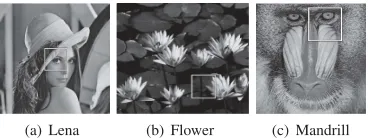
An arbitrarily chosen small square subregion of three images are used during the training to generate high quality filters via GA to reduce the training time. The training images are cropped from the Lena, Flower and Mandrill images as original (basis) images (Figure 1) and exposed to random noise at a given level before each training process.
An initial population with a size of 50 individuals is randomly generated according to the value ranges of each gene. Uniform crossover is used for recombination after choosing 2 parents using tournament selection with a tour size of 4. The traditional mutation operator randomly perturbs an allele with a probability of 1/individual-length. The best individual is maintained while the rest of the population is replaced by the new individuals. A run is terminated after 1000 generations. To obtain the best filter, GA is run with the same parameters and with the same training images for 30 trials. At each trial, a different set of training images is used. Each training image used at a trial is obtained by exposing the basis image to random noise generated using a different random seed at the given level of noise. After termination, the best filter generated having the best fitness from all 30 trials is tested over ten “unseen” images (Fig 2). During the testing phase, each test image is corrupted with various levels of noise ranging from
10%to90%for each trial in a similar manner as the training images.
We performed 3 different sets of experiments. In the first set of experiments, level of salt and pepper noise is fixed and the performance of different median filters are compared along with the generated filter. In the second set of experiments, the best filter achieved for various noise levels is tested on test images and the results are compared to those of well-known filters from the literature. Finally, an entirely different type of noise, namely Gaussian noise, is handled with the filter which was trained to eliminate impulse noise. The goal is to evaluate the generality level of the filter evolved by GA.
B. Comparison of Filters at a Fixed Noise Level
In the first set of our experiments, level of noise is fixed as
(a) Lena (b) Flower (c) Mandrill
Fig. 1. Cropped part of each image that is taken to form the training set.
(a) Camera (b) Bridge (c) Peppers (d) Airplane (e) Mandrill
(f) Lena (g) Goldenhill (h) Boat (i) Parrot (j) Reptile
Fig. 2. Test images.
and shape error criteria, the generated filter gave better results across all images. According to MAE criteria, generated filter is always better than almost all median filters, except for the Reptile image, for which the3×3median filter gave a better result. According to brightness error criterion, performance of the generated filter is the worse. The 3×3 median filter performs well with respect to this criterion as compared to the other median filters of size 4×4 and 5×5. In most of the cases, the generated filter is better than the large size median filters but slightly worse than the 3×3 median filter. In the overall, the generated filter delivers a better performance than the median filters of different sizes and the best performing median filter is of size3×3.
C. Comparison to Previously Proposed Approaches
The second set of experiments is organized with the goal of comparing the performance of our approach to the previously proposed ones. In the literature, performance of most of the approaches are reported with respect to the MSE values on 3 images: Lena, Mandrill and Peppers. The performance of gen-erated filters are evaluated on the corrupted versions of those images with 9 different levels of noise: {10%, 20%,.., 80%, 90%}. The same noise levels are used during the training pro-cess. The performance of each filter produced for a given noise level during the training is also tested across images corrupted with other noise levels. In general, the noise level is not known prior to reconstruction of an image. On average, it has been observed that the filter obtained by using training instances with 60% noise yields a better performance (Fig 3). Please note that, the results for all noise levels are not shown due to lack of space. However, Table III summarizes the results for the filter trained on images with 60%noise (the best performing evolved filter) are presented and compared to other well established methods from the literature: Anfis-based Impulsive
noise removing Filter (AIF) [2], Spatial Median Filter(SMF) [27], Iterative Median Filter (IMF) [29], Progressive Switching Median Filter (PSM) [29], Signal Dependent Rank Order Mean Filter (SDROM) [1], Two-state Recursive Signal Dependent Rank Order Mean Filter (SDROMR) [1], Impulse Rejecting Filter (IRF) [4], Non-Recursive Adaptive-Center Weighted Me-dian Filter (ACWM) [5] Recursive Adaptive-Center Weighted Median Filter (ACWMR) [5], Center Weighted Median Filter (CWM) [17], Y¨uksel’s Anfis based filter (Y ¨UKSEL) [30], Russo’s fuzzy filter (RUSSO) [23] and Histogram Based adaptive fuzzy filter (HAF) [28].
Each approach is ranked from 1 (best) to 14 (worst) based on the MSE values for each resultant image, then the average ranking of each approach is provided. As expected, in most of the cases, a filter obtained after training on instances at a given noise level is more successful in eliminating noise from an image corrupted at the same noise level. Our filter does not give the best results among all the filters, but if we look at the results of each for their generated noise level, it can be observed that our method gets a rank in the top 3 or 4 filters among the state-of-the-art filters from the literature.
D. Eliminating Gaussian Noise
[image:4.595.136.466.177.336.2]TABLE I. PERFORMANCE COMPARISON OF OUR FILTER(OBTAINED AFTER TRAINING USING THE SMALL IMAGES WITH20%SALT AND PEPPER NOISE) AND MEDIAN FILTERS WITH RESPECT TO DIFFERENT METRICS BASED ON MEAN VALUES(AVERAGED OVER30RUNS). MAE: MEANABSOLUTEERROR,
MSE: MEANSQUAREDERROR, SE: SHAPEERROR, BE: BRIGHTNESSERROR
Err
or
T
ype
Method Camera Bridge Peppers Air
plane
Mandrill Lena Goldenhill Boat Parr
ot
Reptile
MAE
GA(20%) 5.27 8.55 2.53 2.90 10.72 2.52 3.95 3.67 3.05 4.68
3×3 5.94 9.76 2.80 3.21 11.74 2.79 4.58 4.22 3.36 4.01
4×4 8.19 12.48 4.41 5.20 14.43 4.53 6.15 6.17 4.69 5.99
5×5 7.77 12.47 3.55 4.52 14.69 3.81 5.99 5.76 4.29 5.44
MSE
GA(20%) 169.86 184.34 31.21 47.02 300.25 31.91 49.56 58.84 77.08 79.06
3×3 276.02 289.72 78.96 110.46 392.60 79.87 111.79 123.17 125.00 119.74
4×4 414.40 374.73 131.34 191.47 491.62 120.77 122.13 176.19 150.92 160.71
5×5 373.53 373.07 67.40 128.10 502.10 79.73 121.17 151.44 141.83 131.49
SE
GA(20%) 46.61 49.64 18.21 21.77 64.66 18.34 25.04 26.18 31.40 28.14
3×3 59.91 62.90 31.03 35.58 75.18 30.59 37.89 38.74 40.50 38.60
4×4 64.48 64.32 30.40 36.24 77.68 29.15 34.36 38.81 39.89 37.24
5×5 62.85 64.06 24.68 32.54 79.06 25.94 34.97 37.84 40.10 35.19
BE
GA(20%) 0.16 0.23 0.16 0.23 0.32 0.03 0.06 0.20 0.13 1.16
3×3 0.58 0.39 0.11 0.20 0.43 0.17 0.21 0.12 0.09 0.09
4×4 1.28 0.78 0.12 0.21 0.64 0.31 0.41 0.17 0.29 0.21
5×5 1.20 0.90 0.25 0.14 0.72 0.40 0.51 0.04 0.26 0.49
TABLE II. AVERAGE RANK OF EACH FILTER OVER ALL NOISY IMAGES
Method Lena Mandrill Peppers Method Lena Mandrill Peppers
Our Method(10%) 15,44 15,00 14,11 SMF(3×3) 17,56 17,11 16,44
Our Method(20%) 12,56 12,33 11,11 PSM 12,22 10,89 10,89
Our Method(30%) 10,78 11,33 9,44 SDROM 18,78 17,33 19,11
Our Method(40%) 8,33 9,67 7,67 SDROMR 11,56 11,33 12,33
Our Method(50%) 9,44 9,89 8,78 IRF 17,11 16,11 17,11
Our Method(60%) 7,56 8,67 6,67 ACWM 17,22 15,22 17,56
Our Method(70%) 10,67 10,56 9,56 ACWMR 9,78 7,89 10,11
Our Method(80%) 9,11 9,33 10,22 CWM 20,89 19,89 20,78
Our Method(90%) 11,44 10,67 13,22 Y ¨UKSEL 7,56 7,56 13,00
AIF 1,00 1,00 1,00 RUSSO 11,56 18,44 12,22
IMF 10,44 10,78 9,67 HAF 2,00 2,00 2,00
TABLE III. AVERAGE RANK OF DIFFERENT FILTERS,WHICH ARE OBTAINED USING DIFFERENT APPROACHES,BASED ON THEIR PERFORMANCES WITH RESPECT TOMSEOVER DIFFERENT LEVELS OF NOISE. EACH FILTER IS USED TO ELIMINATE SALT AND PEPPER NOISE FROM THELENA, MANDRILL AND
PEPPERS IMAGES,EACH CORRUPTED WITH NINE DIFFERENT LEVELS OF NOISE FROM10%-90%AND RANKED ACCORDINGLY.
Method Lena Mandrill Peppers Method Lena Mandrill Peppers
GA(60%) 5.33 6.00 4.56 IRF[4] 10.44 9.78 10.33
AIF[2] 1.00 1.00 1.00 ACWM[5] 10.67 9.11 10.89
IMF[29] 6.78 6.89 5.67 ACWMR[5] 5.67 5.11 5.67
SMF- 3x3 [27] 10.44 10.11 9.67 CWM[17] 13.67 13.11 13.56
PSM[29] 7.56 6.89 6.33 Y ¨UKSEL[30] 5.00 4.56 8.22
SDROM[1] 12.11 11.00 12.33 RUSSO[23] 7.11 12.11 7.33
SDROMR[1] 7.22 7.33 7.44 HAF[28] 2.00 2.00 2.00
Gaussian noise is applied on all images. The variance of the Gaussian noise is varied from10%to90%. Subsequently, the 3 by 3 median filter and the selected filter which is trained at
60%noise level is applied to all those images and the results are recorded according to mean-squared-error criteria. The test results show that, our method also can eliminate Gaussian noise and achieves significantly better results than the median filter for all images and noise levels (Table IV).
V. CONCLUSION
In this study, an evolutionary approach is used to generate a noise filter which is based on soft mathematical morphology. Elimination of noise while preserving details as much as possible is achieved by using a representation which allows multi-stage filters with a wide range of structuring elements and by combining four different objectives in the fitness function. We generated a filter which is enabled to handle different levels of noise and compared its performance to the best known filters from the literature. Our filter turned out to
be one of the top filters with respect to the MSE criterion. Although that filter was specifically tailored for impulsive noise, tests over Gaussian noise added images showed that it is also successful in eliminating this type of noise regardless of its level. The evolved filter outperformed the Median filter almost for all images and noise levels tested. This work shows that using evolution to generate “resuable” filters to eliminate noise is a viable approach. Moreover, the evolutionary process is capable of learning from small instances how to eliminate noise which then can be applied to large unseen instances.
REFERENCES
[1] Abreu, E., Lightstone, M., Mitra, S.K., Arakawa, K., (1996), A new efficient approach for the removal of impulse noise from highly cor-rupted images, Image Processing, IEEE Transactions on , vol.5, no.6, pp.1012,1025, Jun 1996, doi: 10.1109/83.503916.
[2] Bes¸dok E. (2004), A new method for impulsive noise suppression from highly distorted images by using Anfis, Engineering Applications of Artificial Intelligence, 17, pp. 519-527.
Fig. 3. Pairs of Lena images, corrupted with noise levels from10%−90%(up) and reconstructed using an evolved filter trained at a60%noise level (down).
TABLE IV. COMPARISON OF THE AVERAGE VALUES OFMEDIANFILTER(3×3)AND SELECTED FILTER RESULTS FOR EACH IMAGE(MSECRITERIA) GIVEN AGAUSSIANNOISE
Image Our Method Median Filter Image Our Method Median Filter
Camera 1345.01 3895.39 Lena 1104.35 3783.05
Bridge 1409.56 3921.38 Goldhill 1110.90 3771.69
Peppers 1104.59 3690.05 Boat 1168.55 3786.48
Airplane 1070.35 3472.62 Parrots 1159.43 3817.20
Mandrill 1527.03 4208.30 Reptile 1297.67 4020.27
[4] Chen, T., Wu, H.R., (2000), A new class of median based impulse rejecting filters. IEEE International Conference on Image Processing 1, pp. 916-919.
[5] Chen, T., Wu, H.R., (2001), Adaptive impulse detection using center-weighted median filters, Signal Processing Letters, IEEE , vol.8, no.1, pp.1,3, Jan. 2001, doi: 10.1109/97.889633.
[6] Chun-hui Z., Gang-jian L., Hai-chun N. (2006), Optimization of soft morphological filter based on tabu search. In Proceedings of the First International Conference on Innovative Computing, Information and Control (pp. 611-614), Beijing, China.
[7] Chunhui Z., Shenghe S., Junying H. (2000), Optimization of soft morphological filters by simulated annealing. In Proceedings of the 5th International Conference on Signal Processing (pp. 494-498), Beijing, China.
[8] C¸ ivicio˘glu P. (2007), Using neighborhood-pixels-information and AN-FIS for impulsive noise suppression, Int. J. Electron. Commun. (AE ¨U), 61, pp. 657 - 664.
[9] Harvey N.R., Marshall S. (1994), Using genetic algorithms in the design of morphological filters. In J. Serra, Pierre S., Mathematical Morphology and Its Application to Image Processing (pp. 53-59), France: Kluwer Academic Publishers.
[10] Jayasree, P.S., Kumar, P., A fast novel algorithm for salt and pepper impulse noise removal using B-Splines for finger print forensic images, 2013 IEEE Second International Conference on Image Information Processing (ICIIP), vol., no., pp.427,431, 9-11 Dec. 2013.
[11] Jelodar M.S., Fakhraie S.M., Ahmadabadi M.N. (2006), Two-stage morphological filter design using genetic algorithm. In Proceedings of the IEEE International Conference on Engineering of Intelligent Systems (pp. 129-133), Islamabad, Pakistan.
[12] Koskinen L., Astola J., Neuvo Y. (1991), Soft morphological filters. In Proceedings of the SPIE Symp. Image Algebra and Morphological Image Processing (pp. 262-270), San Diego, CA.
[13] Kuosmanen P., Astola J. (1995), Soft morphological filtering. Journal Mathematical Imag. Vision, 5(3), 231-262.
[14] Kuosmanen P., Koivisto P., Huttunen H., Astola J. (1995), Shape preservation criteria and optimal soft morphological filtering, J. Math. Imag. Vision, 5(4) pp. 319-335.
[15] Lin T.C. (2008), Progressive decision-based mean type filter for image noise suppression, Computer Standards Interfaces, 30, pp. 106-114.
[16] Matheron G. (1975), Random sets and integral geometry. New York: Wiley.
[17] Muneyasu, M., Nishi, N., Hinamoto, T., (2000), A new adaptive center weighted median filter using counter propagation networks. Journal of the Franklin Institute 337, pp.631-639.
[18] Ozcan E. (2005), Memetic algorithms for nurse rostering. Lecture Notes¨ in Computer Science, 3733, pp. 482-492.
[19] Ozcan E., Mohan C. K. (1997), Partial shape matching using genetic¨ algorithms. Pattern Recognition Letters, 18, pp. 987-992.
[20] Ozcan E., Onbasioglu E. (2007), Memetic algorithms for parallel code¨ optimization. International Journal of Parallel Programming, 35(1), pp. 33-61.
[21] Pitas I., Venetsanopoulos A. N. (1990), Nonlinear digital filters -principles and applications. Boston: Kluwer Academic Publisher.
[22] Russo F. (2004), Impulse noise cancellation in image data using a two-output nonlinear filter, Measurement, 36, pp. 205-213.
[23] Russo, F., Ramponi, G., (1996), A fuzzy filter for images corrupted by impulse noise. IEEE Signal Processing Letters 6 (3), pp. 168-170.
[24] Serra J. (1982), Image analysis and mathematical morphology (Vol.I), London: Academic Press.
[25] Serra J. (1986), Introduction to mathematical morphology. Comp. Vision Graph. Image Proc., 35(3), pp. 283-305.
[image:6.595.303.556.432.753.2][27] Tukey, J.W., (1974), Nonlinear (nonsuperposable) methods for smooth-ing data, Congress Records EASCON’74, 673
[28] Wang, J.H., Liu, W.J., Lin, L.D., (2002), Histogram-based fuzzy filter for image restoration. IEEE Transactions on Systems, Man, and Cyber-netics, Part B 32 (2), pp. 230-238.
[29] Wang, Z., Zhang, D., (1999), Progressive switching median filter for the removal of impulse noise from highly corrupted images. IEEE Transactions on Circuits and Systems-II: Analog and Digital Signal Processing, 46 (1), pp. 78-80.
[30] Y¨uksel M.E., Bas¸t¨urk A. (2003), Efficient Removal of Impulse Noise from Highly Corrupted Digital Images by a Simple Neuro-Fuzzy Operator, Int. J. Electron. Commun. (AE ¨U), 57(3), pp. 214-219. [31] Zhong, L., Cho, S., Metaxas, D., Paris, S., Wang, J., Handling Noise