Elliott Kendrick Levi
A Thesis Submitted for the Degree of PhD
at the
University of St Andrews
2017
Full metadata for this item is available in
St Andrews Research Repository
at:
http://research-repository.st-andrews.ac.uk/
Please use this identifier to cite or link to this item:
http://hdl.handle.net/10023/16690
Elliott Kendrick Levi
This thesis is submitted in partial fulfilment for the degree of Doctor
of Philosophy
at the
University of St Andrews
by me, and that it is the record of work carried out by me, or principally by myself in collaboration with others as acknowledged, and that it has not been submitted in any previous application for a higher degree.
I was admitted as a research student in September 2012 and as a candidate for the degree of Doctor of Philosophy in September 2012; the higher study for which this is a record was carried out in Heriott-Watt University between 2012 and 2013 and in the University of St Andrews between 2013 and 2016.
I, Elliott Kendrick Levi, received assistance in the writing of this thesis in respect of language, grammar, spelling and syntax, which was provided by Doctor Peter Kirton
Date signature of candidate
2. Supervisor’s declaration:
I hereby certify that the candidate has fulfilled the conditions of the Resolution and Regulations appropriate for the degree of Doctor of Philosophy in the University of St Andrews and that the candidate is qualified to submit this thesis in application for that degree.
Date signature of supervisor
3. Permission for publication:
In submitting this thesis to the University of St Andrews I understand that I am giving permission for it to be made available for use in accordance with the regulations of the University Library for the time being in force, subject to any copyright vested in the work not being affected thereby. I also understand that the title and the abstract will be published, and that a copy of the work may be made and supplied to any bona fide library or research worker, that my thesis will be electronically accessible for personal or research use unless exempt by award of an embargo as requested below, and that the library has the right to migrate my thesis into new electronic forms as required to ensure continued access to the thesis. I have obtained any third-party copyright permissions that may be required in order to allow such access and migration, or have requested the appropriate embargo below.
The following is an agreed request by candidate and supervisor regarding the publication of this thesis: PRINTED AND ELECTRONIC COPY
Embargo on abstract and Chapter 5 of print and electronic copies for a period of 1 year on the following ground: Publication would preclude future publication
Date signature of candidate signature of supervisor
Please note initial embargos can be requested for a maximum of five years. An embargo on a thesis submitted to the Faculty of Science or Medicine is rarely granted for more than two years in the first instance, without good
justification. The Library will not lift an embargo before confirming with the student and supervisor that they do not intend to request a continuation. In the absence of an agreed response from both student and supervisor, the Head of School will be consulted. Please note that the total period of an embargo, including any continuation, is not expected to exceed ten years.
“They’ve done studies, you know. 60% of the time, it works every time.”
Abstract
This thesis covers open quantum systems and information transfer in the face of dissipation and disorder through numerical simulation.
In Chapter 3 we present work on an open quantum system comprising a two-level system, single bosonic mode and dissipative environment; we have included the bosonic mode in the exact system treatment. This model allows us to gain an un-derstanding of an environment’s role in small energy transfer systems. We observe how the two-level system-mode coupling strength and the spectral density form char-acterising the environment interplay, affecting the system’s coherent behaviour. We find strong coupling and a spectral density resonantly peaked on the two-level sys-tem oscillation frequency enhances the syssys-tem’s coherent oscillatory dynamics.
Chapter 4 focusses on a physically motivated study of chain and ladder spin geometries and their use for entanglement transfer between qubits. We consider a nitrogen vacancy centre qubit implementation with nitrogen impurity spin-channels and demonstrate how matrix product operator techniques can be used in simulations of this physical system. We investigate coupling parameters and environmental decay rates with respect to transfer efficiency effects. Then, in turn, we simulate the effects of missing channel spins and disorder in the spin-spin coupling. We conclude by highlighting where our considered channel geometries outperform each other.
Acknowledgements
The last four years have been filled with the typical highs and lows that accompany a PhD. Despite it being common knowledge that there will be good days, weeks and months and bad days, weeks and months, it is nearly impossible to prepare a PhD student for how tough those bad periods can be. However we don’t go through them alone.
I’d first like to thank my supervisor, because without Brendon Lovett this the-sis would not exist. I am happy that I made the right choice in him and working with him has been an enjoyable way to achieve what I have. It could never be over-stated, the effect that a good supervisor has on their students. Thanks need also go to my collaborators, Elinor Irish and Peter Kirton, whose experience and knowledge helped me reach the lofty heights of published academic authorship. The academic and administerial staff of the CM-CDT have provided help, advice and phenomenal organisational skills and ensured that no place I ever work will be run as well or by such friendly people.
A person can’t exist on work alone and I’ve made a lot of friends in the time doc-umented by this thesis. Too many to name, it would be unfair on those I mistakenly forgot. Those of you who contributed to keeping me occupied, whether it be a trip to the cinema, a board game night, cake day or something else entirely, know who you are. I hope you know you were a welcome and necessary part of what I’ve been through, torment and all.
Publications
[1] Coherent exciton dynamics in a dissipative environment maintained by an off-resonant vibrational mode E. K. Levi, E. K. Irish, and B. W. Lovett, Phys. Rev. A 93, 042109 (2016).
Contents
Declaration of Authorship i
Abstract iii
Acknowledgements iv
1 Introductions and the way forward 1
1.1 Thesis overview . . . 2
1.1.1 Open quantum systems theory . . . 2
1.1.2 Maintenance of coherent dynamics in a dissipative environment 3 1.1.3 Entanglement transfer spin channel geometries . . . 3
1.1.4 Entanglement routing . . . 4
1.2 Open Quantum Systems . . . 4
1.2.1 Photosynthesis . . . 5
1.2.2 Quantum state transfer . . . 9
1.2.3 Nitrogen vacancy centres . . . 11
1.2.4 Entanglement distribution . . . 12
2 Open quantum systems theory 15 2.1 Dynamical density matrices . . . 17
2.1.1 Born-Markov master equation . . . 19
2.1.2 Lindblad master equation . . . 21
2.2 Characterising environments . . . 24
2.2.1 Phenomenology . . . 25
2.2.2 Derivation . . . 26
2.2.3 Markovianity and methods . . . 29
2.3 Matrix product operator formalism . . . 30
2.3.1 The Schmidt and singular value decompositions . . . 30
2.3.2 A matrix product state . . . 32
2.3.3 Expressing density matrices . . . 34
2.3.4 The Suzuki-Trotter expansion . . . 35
2.3.5 Time-evolving block decimation . . . 36
2.4 Simulations . . . 39
2.4.1 Probability . . . 40
2.4.2 Entanglement of formation . . . 40
3 Maintenance of coherent dynamics in a dissipative environment 43
3.1 The model . . . 45
3.1.1 The Fulton-Gouterman transformation . . . 47
3.1.2 Add the bath . . . 49
3.2 Derived master equation . . . 49
3.2.1 The interaction picture . . . 50
3.2.2 Changing bases . . . 50
3.2.3 Moving to the interaction picture . . . 52
3.2.4 Generation of the master equation . . . 53
3.2.5 Characterising the environment . . . 58
3.3 Computational implementation . . . 59
3.4 Results . . . 61
3.4.1 Preliminary result . . . 61
3.4.2 An Ohmic environment . . . 63
3.4.3 Super-Ohmic environments . . . 64
3.4.4 Analysis . . . 64
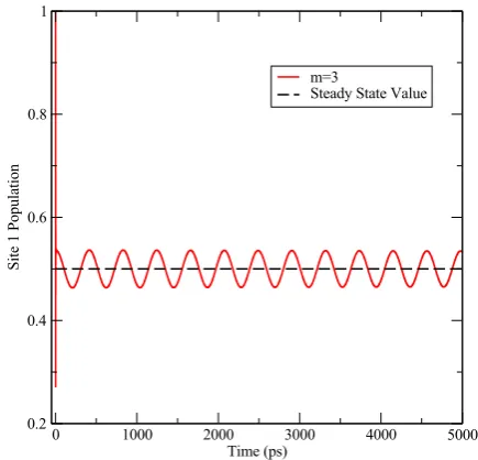
3.4.5 Long time behaviour . . . 67
3.4.6 A resonant Lorentzian environment . . . 68
3.4.7 A sub-resonant Lorentzian environment . . . 70
3.5 Concluding remarks . . . 70
4 Entanglement transfer spin channel geometries 72 4.1 Our model . . . 73
4.1.1 Our method . . . 75
4.1.2 Implementation . . . 76
4.2 Computational solution . . . 78
4.3 Results . . . 81
4.3.1 Spin coupling and NV splitting . . . 81
4.3.2 Channel length . . . 83
4.3.3 Channel decay rate . . . 84
4.3.4 Missing spins . . . 85
4.3.5 Placement disorder . . . 89
4.4 Concluding remarks . . . 90
5 Entanglement routing 93 5.1 Spin network router . . . 94
5.2 Single sender routing . . . 99
5.2.1 Eigenstate population amplitude exploitation . . . 101
5.3 Two-sender routing . . . 107
5.3.1 Two site toy model and parabolic coupling . . . 108
5.3.2 Uniform coupling network routing . . . 114
5.4 Concluding remarks . . . 122
6 In closing 123 6.1 An overview . . . 123
1
Introductions and the way forward
T
HEtherefore an open system. In general, systems are ‘things’; ecosystems, cars,universe, as a whole, is a closed system and every sub-system within it iscomputers, atoms. Closed systems are contained, so only the system’s parts dictate its behaviour whereas an open system has some interaction with external entities. To fully describe the behaviour of an open system the external environment must be considered. Definitions of closed and open systems do vary slightly with the scale of the physics being studied, for instance classically closed means no forces are exerted from outside and matter and energy are conserved. Thermodynamically a closed system permits energy flow but no matter, when both matter and energy exchanges are absent it would be an isolated system (similar to a closed classical mechanical system). And in standard quantum mechanics an isolated thermodynamic system is usually termed a closed system; one governed by the Schrödinger equation where no information (meaning energy or matter) can enter or leave the system (see Fig. 1.1). Conversely then, generally an open quantum system (OQS) is free to exchange infor-mation and energy with its environment.
FIGURE1.1: Schematic illustrations of closed and open quantum sys-tems. A closed system (left) where only the circular blue ‘system’ is considered and the environment is either functionally or approxi-mately uncoupled; information (such as energy or particles) is con-served within the system. The open system (right) is now in contact with its environment and in general information can flow between them. As such, information in the blue system is now not conserved.
the work within to serve. We concern ourself with investigations of a few different aspects of the OQS jigsaw; extending methods, considering novel system realisations and subverting expectations with regards to intuitive concepts.
1.1
Thesis overview
F
AIRLYout over the period of study and comprising extra material to support it. Wetraditionally this thesis is split into chapters covering the work carriedhave already introduced the highest level motivation and intent for the work in this chapter. We shall continue to outline and explore the thesis here, introducing in more detail the concepts associated with OQSs and what we intend to do.
1.1.1 Open quantum systems theory
state vectors due to the latter’s inability to describe OQSs. The environment itself, although often vastly complex and numerically intractable must be handled in some way and this will be discussed. We will detail a master equation formalism for mod-elling an OQS in contact with an environment and the matrix product operator ap-proach to solving a master equation. Finally we cover a measure of entanglement which we employ in later chapters to quantify system performance.
1.1.2 Maintenance of coherent dynamics in a dissipative environment
Chapter 3 is our first chapter of original work (forming the basis for Publication 1) and concerns the interplay between a system and its environment when part of that environment is being considered as a component of the system. This is a novel exam-ple of extending current methods to reduce the level of approximation used to treat environments and the precise formulation of the model could be thought of as a toy for photosynthetic systems. Making use of a symmetry-exploiting transformation, a ‘microscopic’ (as opposed to phenomenological) master equation is derived and a computational solution of it described in order to describe the system exactly. We show that exact treatment of this included environmental component leads to inter-esting behaviour, in that by tuning its coupling within the system one can change the coherent properties of the system. An analytic interpretation of this effect is presented and its relation to the description of the environment is explored.
1.1.3 Entanglement transfer spin channel geometries
two kinds of channel in the face of an imperfect hypothetical manufacturing process. Part of our results will be obtained using a matrix product operator approach, em-ploying it beyond the usual application to theoretical models and performing it in such a way as to extend what sized systems can be studied. We find that there is, once again, an interplay between the environment and system affecting coherent dy-namics. Further, when the manufacturing imperfections are considered it is possible for a ladder to outperform a chain in terms of entanglement distribution, but perhaps not to the degree that was expected when one considers the extra couplings present in a ladder geometry.
1.1.4 Entanglement routing
Born of the considerations of the preceding chapter, Chapter 5 asks: if we can dis-tribute entanglement between pairs can we send it in an addressable way and, if so, can multiple transmission processes coexist? Relaxing the physical restrictions slightly and considering this more as a question answered with a physically inspired toy model, we consider 2D grids of spins (a superset of the ladder and chain geome-tries considered previously) with sender and receiver qubits coupled to them. In con-sideration of what is possible we return to an idea investigated in earlier work asso-ciated with quantum state transfer, namely eigenmode transport, showing that with this it is indeed theoretically possible to route entanglement from a sender. Using this process we can distinguishably route entanglement, initially between the sender and an ancilla, such that at some time later only a desired receiver (one of multiple coupled to the spin network) is entangled with the ancilla. Then, extending this, we incorporate a second sender-ancilla pair and show that concurrent routing events can be realised with similar distinguishability.
1.2
Open Quantum Systems
H
AVINGwe are interested in doing this work. It would be fair to say that the theoreticalseen what will be included in this thesis let us go back and look at whybody physics, in the sense that we currently cannot hope to deal with all of the states of a system and its surrounding environment exactly. As an aside, throughout this thesis the terms ‘environment’, ‘bath’ and ‘surroundings’ will be used more or less interchangeably to describe the same thing. With an OQS the stance is often adopted that, as we are not interested in the state of the environment, it is assumed to be of a simplified form that is easier to manage and can approximate averaged behaviours or weakly coupled parameter limits. But there are cases when the environment has been shown to be important, such as with the revelation of the quantum coherent processes in photosynthetic systems [3–5], which we will now discuss.
1.2.1 Photosynthesis
Despite being at the forefront of a lot of experimental [6–9] and theoretical [10–19] inquiry we have still only part knowledge as to the sources of the coherence and how precisely it enhances the transport efficiency of the photosynthetic process [20–22]. Some of the big open questions in the field include how to best model complicated bi-ological structures accurately, whetherex-vivoexperiments displaying coherence un-der coherent light sources can shed light onin-situoperation [23–25] and whether the coherence observed is electronic, vibrational or some mixture [26–28].
a reaction centre is comprised of two closely spaced chromophores.
FIGURE 1.2: A schematic impression of a photosynthetic unit prised of chromophores (collectively forming the light harvesting com-plex), the reaction centre (where the chemical process is initiated) and
a surrounding protein environment.
There are a range of chromophores (like chlorophylls or carotenoids) with differ-ent properties; generally each is responsive to a differdiffer-ent part of the electromagnetic spectrum and can also serve to protect the organism by absorbing light that would otherwise be damaging to the plant [31]. In many instances chromophores are sur-rounded by a protein basket, referred to together as a pigment-protein complex, and since changes to the protein’s conformation also affect the chromophore the spectral properties of the latter can be tuned [32]. A chlorosome is another pigment structure that has been observed in LHCs, these are large collections of chromophores bound together without protein baskets [33].
FIGURE1.3: Four representations of the Fenna-Matthews-Olsen LHC.
The ribbon view shows a biological representation of the protein rib-bons surrounding the green chromophores. The site basis identifies the individual chromophores which, in the case of this organism, are chlorin rings. The excitonic basis is a physical representation of the density clouds (represented as different colours) of the single excita-tion associated with each chromophore. Finally the atomic view shows how densely packed this LHC is and just how many constituent atoms
there are to consider. Figure obtained from Ref. [34].
As previously mentioned, it is known that the exciton travels through the chro-mophores to reach the reaction centre, but the precise mechanism by which this occurs is unknown. The energy dynamics can be probed using spectroscopic techniques and commonly used now in photosynthetic studies is 2D electronic spectroscopy. This uses four-wave-mixing and elicits third order correlations in the form of an emitted signal field resulting from the laser-sample interaction [35]. This technique repre-sents a step forward in our probing technologies as one of its big advantages is that the spectrum obtained is in terms of amplitudes (as opposed to intensities) so the sys-tem’s quantum phase is directly accessible; this means that quantum coherence can be observed.
of the other). Starting with energies we shall consider the inter-chromophore elec-tronic coupling strength and the chromophore interaction strength. When bath-chromophore beats electronic coupling, bath-chromophore localised electronic states make the most logical basis states, with a perturbative treatment of inter-chromophore exci-tonic coupling; this approach is called Förster theory [36]. This limit can be thought of as a hopping limit, where the electron exists on one site at a time, and hops between chromophores. In the opposing limit, when the electronic coupling is greater than bath-chromophore interactions, a localised electron is not a convenient state descrip-tion as it may delocalise across chromophores; now the bath-chromophore couplings are treated perturbatively to produce a quantum master equation, such as in Redfield theory [37].
FIGURE1.4: Illustrations of electronic behaviour in the a) hopping and b) delocalised regimes of chromophoric energy transfer.
be to have strong inter-chromophoric couplings so again we see an understandable equivalence.
Whilst there are systems that these limiting coupling and/or time scale regimes can describe there are also a large number of cases where the parameters fall into in-termediate or competing regimes. Theoretical consideration here is hampered due to the inapplicability of common perturbative or ‘weak coupling’ approaches because of the lack of vanishingly small parameters. In order to investigate the regime where chromophoric coupling is of the same scale as chromophore-protein coupling it is worth noting that whilst precise models of whole LHCs can elucidatein situ perfor-mance they tend to be computationally expensive and may produce a lot of informa-tion. As we are still at a stage of understanding where the mechanisms themselves are still in question, it can be physically instructive to proceed with studies of smaller systems or more manageable toy models. In doing so approximations are made that reduce the possibility of quantitative comparisons with real systems, however the qualitative, physical conclusions drawn from such work can help move forward our understanding of basic governing principles. Chapter 3 contains work that has been motivated by such thinking, taking a system that whilst not quantitatively represen-tative does capture the essence of several physical systems where there is a complex interplay between system and environment.
1.2.2 Quantum state transfer
implementation will exist inside (or possibly on top of) a crystalline environment, constantly experiencing phononic vibrations similar to the protein baths of our previ-ous example. We can also still use many of the already established OQS methods and techniques then to investigate this novel application of quantum mechanics.
The use of spin-1/2 chains as QST channels is a well covered subject [44–46] and has been extended to dual- [47] and multi-rail [48, 49] spin chains. The intent is simple, take an arbitrary quantum state|ψi =a|↑i+b|↓idefined on one sending qubit and transfer it to a second receiving qubit whilst maintaining high fidelity. It is this last point, maintenance of high fidelities, that motivates study as this is clearly an area where understanding how a system interacts with its environment can pave the way for new device constructions and scientific advancements.
In Fig. 1.5 we present the basic structure required for such a QST process. There are a number of ways QST can be implemented along a chain such as this, including modulating spin energies and controlling couplings between them [50–55]. The way we consider here is a minimal control approach, in so far as the chain is dark and control of the process is governed only by the state qubits themselves. As we have presented it in Fig. 1.5 the system is uniform in spin placements (spacings) but in general the idea of dark spin wiring that we will introduce does not need this to be the case.
FIGURE1.5: Illustration of a spin-1/2 chain quantum state transfer sys-tem. The sender qubit is initialised in an arbitrary state which, as the
system evolves, is transferred to the receiving qubit.
the Zeeman splitting of the qubits match it; this is represented in Fig. 1.6. With pertur-bative state qubit-chain interactions one is able to solve the eigen-system of the iso-lated chain and obtain its eigenvalues. We can restrict ourselves to considering only the single excitation states of the chain as transport eigenmodes as the sender qubit can only introduce one excitation; this assumes the chain is initially all spin down. Theoretically this operating mode can transport the state with very high fidelity as interference due to phase effects of differing transfer speeds through different eigen-states of the chain are minimised.
FIGURE 1.6: A schematic of the eigenmode tunnelling mechanism of spin channel wiring. Provided the qubit-chain coupling is weak com-pared to the intra-chain coupling then transfer via only one mode oc-curs which is free from interference effects and thus is of high fidelity.
1.2.3 Nitrogen vacancy centres
(room temperature) electron and nuclear spin decoherence times [58, 59]. They are also amenable to precise measurement and manipulation [60] which has led to an experimentally realisable set of universal quantum operations [61, 62]. And their flu-orescence properties make them experimentally convenient ways of interfacing be-tween optics and solid state schemes.
FIGURE 1.7: a) A diamond unit cell with one missing carbon atom and one nitrogen atom substitution forming an NV. b) A single sub-stitutional nitrogen atom in a diamond unit cell which is known as a
nitrogen impurity.
An NV has a (ground) multi-level electronic structure as depicted in Fig. 1.8, clearly not a neat two level system, however we can control it as if it were, isolating two levels [61, 63]. The system can be initialised in|↓i through optical pumping to excited levels and non-radiative decay via the singlet state [64]. A magnetic field can split the degenerate ms = ±1 levels [60] and we can define the ms = 0 and
ms = 1as |↓iand|↑i respectively giving us a well defined two level basis. Finally
with microwave pulses the coherent control of|↓iand|↑ican be implemented [65].
1.2.4 Entanglement distribution
FIGURE1.8: The simplified electronic structure of an NV with the
rel-evant computational basis levels labelled. Application of a magnetic field causes splitting of the degenerate triplet levels. Optical pumping achieves an initialised down state and through microwave control the
up state can be populated coherently.
distribution where perfect fidelity transfer is not necessarily required. Whilst many quantum frontier implementations are still a little way off, one constant theme ap-pears to be entanglement; in realisations of quantum computing [66, 67], cryptogra-phy [68, 69] and metrology [70, 71] there is clearly a need for the creation of entangled states.
Spatially separate parties will likely require access to created entangled states so distribution methods are also important. A major problem with distribution via direct transmission will likely be the noisy transfer environment, however there are ways to circumvent this drawback. For instance, it has been shown theoretically that two distant systems can be entangled via a separable ancilla [72, 73] and experimen-tally realised with photons [74] and Gaussian beams [75, 76]. Another possibility is counterfactual entanglement which is created with no physical interaction [77, 78]. The method of entanglement distillation [79–81] is also promising: a large ensemble of weakly entangled pairs are distributed and through local operations and classical communication are refined into a small ensemble of highly entangled pairs.
2
Open quantum systems theory
C
ONTAINEDniques of open quantum systems (OQSs), specifically for obtaining time de-within this chapter, will be an introduction to the methods andtech-pendent dynamics. We will first highlight the tool used for description of the systems themselves, density matrices, then move onto to how we formulate a description of a system’s evolution using quantum master equations. Finally we shall cover one method for solving a quantum master equation using matrix product operator tech-niques and include details on the measure of entanglement we employ in later chap-ters which becomes our assessment of system performance.
By way of an introduction, consider the difference between pure and mixed states. When a system is in a pure state writing a state vector, or a superposition thereof, is one way of describing it. For example,|Ψi = P
iCi|ii is a superposition
of the basis states {|ii}, these and their superposition are pure states; we have com-plete information about the phase of the basis states. Suppose that we did not have all of this information, but instead we are presented with an ensemble of these sys-tems after undergoing a measurement. Now we have a statistical mixture of the state outcomes that can no longer be represented as a state vector; this is a mixed state.
(or conversely mixedness) of a state is a continuous property measured asTr ρ2. A purity of 1 is perfectly pure and a maximally mixed state of dimensiondhas purity 1/d.
We can freely write a density matrix as
ρ=X
j
pj|ψji hψj|, (2.1)
where we describe a quantum system made up of a statistical mixture of states,|ψji, each weighted by a probability pj. This description encompasses both pure and
mixed states. Returning to our previous expression of a pure state we have only one element in the summation over j, our superposition |Ψi. As our superposition is the state with certainty this impliesp1 = 1and therefore perfect purity. We could
of course expand the superposition in its basis bringing two (one for the ket and one for the bra) summations over the basis: ρ = |Ψi hΨ| → P
ii0CiCi0|ii hi0|. Wheni =i0
we get the diagonal elements ofρwith the probabilities of the basis states, and for all
i6=i0 we obtain the off diagonal ‘coherence’ elements ofρwhich contain information about the phase relation between the states in this basis. Any density matrix can be written in a diagonal basis and whilst this would necessarily change the coherences visibly present between basis states it would not change the purity of the density matrix.
Alternatively let us imagine an experiment in which someone is provided with an ensemble of spin-1/2 particles prepared in the basis{|↑i,|↓i}. Although the dis-tributor of the spins knows the superposition state coefficients (|ψi=α|↑i+β|↓i) the recipients do not and as such, following measurements in the preparation basis, they find themselves in a mixed state with only statistical information available. The re-cipient can use a description like Eq. 2.1, withψj ∈ {↑,↓}and the correspondingpj’s
as the results of their measurements; i.e. given repeated experiments the probability of what the spin orientation would be. They would have only diagonal elements of
properties of their states.
If we write a state vector representation for the system and environment of an OQS, initialised in some coherent way then, should we be able to proceed with a theoretical treatment of this full representation, we would see pure state evolution (assuming the environment is decoupled from the universe). It is commonly the case that it is impossible to fully formulate the complexities of an environment and we must partially trace it out so as to treat only the system
ρS= TrE(ρ). (2.2)
In effect this introduces mixedness into the system description based on how the en-vironment acts on average; the resulting system density matrix ρS is said to be
‘re-duced’. This mixing can be thought of as the environment performing some mea-surement on the state to which an observer is unaware of the result. One can also say that mixedness implies the environment and system have become entangled.
2.1
Dynamical density matrices
P
RESENTEDstate vector, we have to move beyond the Schrödinger equation to an equationthen with an OQS that can no longer in general be described using aof motion for density matrices; such an equation is called a quantum master equation. In the remainder of this chapter we shall endeavour to stick to the convention of using ‘OQS’ to refer to the system we are interested in and the environment it is openly interacting with; technically, combined as this, our OQS is closed. When we use ‘system’ that will be the system part of the OQS. For a full OQS density matrix the equivalent to the Schrödinger equation|ψ˙j(t)i=−iHˆ|ψji
is
˙
ρ(t) =X
j
pj|ψ˙ji hψj|+pj|ψji hψ˙j|=
X
j
pj(−i) ˆH|ψji hψj|+pji|ψji hψj|Hˆ
where we have chosen the convention~= 1as we do throughout this thesis. This is
the Liouville-von Neumann equation [1] and is the most general example of a quan-tum master equation. TheHˆ in Eq. (2.3) is a Hamiltonian for the entire OQS, system and environment, and we have definedLwhich is the Liouville superoperator; a su-peroperator acts on operators to produce operators. The integrated solution of this equation, for the evolution of this density matrix then is
ρ(t) = eLtρ(0), (2.4)
in analogy to the time evolution of a state vector, |ψ(t)i = exp−iHtˆ |ψ(0)i. This clearly is not always a simple equation to write an explicit form of or indeed employ for calculation of ρ(t) due to the complexity of the full OQS Hilbert space and its operators.
Thus far we have considered a Schrödinger picture, where any time dependence resides with state vectors (which extends to the density matrix as well). Let us re-formulate in the interaction picture, where time dependence is shared between states and operators, to progress towards a more tractable form of Eq. (2.3). We start by ac-knowledging the Schrödinger picture OQS Hamiltonian can be split intoHˆ = ˆH0+ ˆHI,
with the first part generally containing isolated system and environment terms (i.e. their energies) and the second describing interactions between the system and its en-vironment. The form of this splitting can vary a lot depending on the system studied, or which techniques are going to be (or have been) applied. Conversion of the den-sity matrix and interaction Hamiltonian to the interaction picture, using the unitary
ˆ
U0 = exp
−iHˆ0t
, follows as
ρ(I)(t) = ˆU0†ρ(t) ˆU0 (2.5) ˆ
HI(I)(t) = ˆU0†HˆIUˆ0, (2.6)
Differentiating Eq. (2.5) we obtain an interaction picture version of Eq. (2.3) [84]
˙
ρ(I)(t) =iHˆ0Uˆ0†ρ(t) ˆU0−iUˆ0†ρ(t) ˆH0Uˆ0+ ˆU0†ρ˙(t) ˆU0
=i
h
ˆ
H0, ρ(I)(t) i
−iUˆ0†
h
ˆ
H, ρ(t)
i
(t) ˆU0
=ihHˆ0, ρ(I)(t) i
−ihHˆ0, ρ(I)(t) i
−ihHˆI(I)(t), ρ(I)(t)i
=−i
h
ˆ
HI(I)(t), ρ(I)(t)
i
. (2.7)
This can also be written in an integral form
ρ(I)(t) =ρ(I)(0)−i
Z t
0 h
ˆ
HI(I)(s), ρ(I)(s)
i
ds. (2.8)
What we have presented so far enables us, broadly speaking, to find the dynam-ics for a composite (system-environment) OQS density matrix. Should we have an OQS that has a simple or convenient analytical form we could use a Liouville-von Neumann equation to obtain an expression for the composite density matrix. Follow-ing from this we can calculate the reduced ρS(t) for the system (which is typically
what we are interested in). But an environment is a tricky thing to deal with on ac-count of its large Hilbert space, so relying on a dynamical description where this is required explicitly and completely (as it is in our descriptions so far) can often create an intractable problem. To tackle this issue we will now approach a derivation of a particular example of an approximate master equation, allowing us to obtain reduced dynamics for ρS(t), without requiring analytic computation of the entire combined
system-environment problem.
2.1.1 Born-Markov master equation
that is system and environment parts acting only on those respective areas and theHI
describing the interaction between them.
We start from the interaction picture Liouville-von Neumann equation and its integral form in Eqs. (2.7) and (2.8), noticing that we can substitute the latter into the former
˙
ρ(I)(t) =−i
ˆ
HI(I)(t), ρ(I)(0)−i
Z t
0 h
ˆ
HI(I)(s), ρ(I)(s)
i
ds
=−ihHˆI(I)(t), ρ(I)(0)i−
Z t
0 h
ˆ
HI(I)(t),hHˆI(I)(s), ρ(I)(s)iids (2.9)
Now we carry out a partial trace over the environment to provide us with the reduced system dynamics
˙
ρ(I)S (t) =−
Z t
0 TrE
h
ˆ
HI(I)(t),hHˆI(I)(s), ρ(I)(s)iids, (2.10)
where we have assumedTrE h
ˆ
HI(I)(t), ρ(I)(0)
i
= 0without loss of generality.
To proceed, we introduce the Born approximation which will allow us to express both sides of Eq. (2.10) in terms of the reduced density matrix; a desirable goal as it lifts the requirement for complete knowledge of the environmental state. It does this by acknowledging a weak coupling approximation between the system and the environment such that the system has a negligible influence on the dynamics of the environment and as such it remains unchanged from its initial stateρE(t) = ρE(0) =
ρE. If we assume, due to this weak coupling, initially we had a separable state, then
we can write for all times thatρ(t)≈ρS(t)⊗ρE(which holds in both the Schrödinger
and interaction pictures). Due to this approximation Born-Markov master equations are sometimes also referred to as weak coupling master equations. Employing the Born approximation allows us to write Eq. (2.10) as
˙
ρ(I)S (t) =−
Z t
0 TrE
h
ˆ
HI(I)(t),hHˆI(I)(s), ρ(I)S (s)⊗ρE ii
ds; (2.11)
Unfortunately Eq. (2.11) is still not time local, it requires information about the history of the reduced density matrix. The Markov approximation helps us with this, stating that the system dynamics at any given instant in time do not have any memory of what happened before, allowing us to make the changeρ(I)S (s)→ρ(I)S (t):
˙
ρ(I)S (t) =−
Z t
0 TrE
h
ˆ
HI(I)(t),
h
ˆ
HI(I)(s), ρ(I)S (t)⊗ρE ii
ds; (2.12)
this form is known as the Redfield equation. This assertion of memoryless dynamics is valid given the physical interpretation that any correlations present in the environ-ment decay over a time scaleτEwhich is much shorter than the dynamical time scale of the system,τS. There is a second simplificationτEτScan imply: the lower limit of the integrand can be extended down to−∞due to the fact that we have rapidly vanishing correlations which imply the integrand will vanish fors τE. Applying
this and the substitutions=t−s0 we reach
˙
ρ(I)S (t) =−
Z ∞
0 TrE
h
ˆ
HI(I)(t),hHˆI(I)(t−s0), ρ(I)S (t)⊗ρE ii
ds0. (2.13)
The Born-Markov master equation we have now in Eq. (2.13) is still very general, but is time local and can generate the reduced system dynamics given an interaction Hamiltonian and the initial environmental and reduced system density matrices. The application of the Markov approximation essentially amounts to a coarse graining of time: we look not at the fast τE but proceed considering dynamics on the scale of
τS. In our application of the Born approximation, although we assumed a weakly coupled, negligibly affected environment that does not mean there are no excitations in it, but when we couple this with the Markov assumption of rapidly decaying bath correlations we see that these excitations are coarse grained out.
2.1.2 Lindblad master equation
entries as probabilities. In Chapter 3 we give a derivation, starting from Eq. (2.13) and using the Hamiltonian and system defined for a particular OQS, to express a Lindblad master equation. Here we proceed to elucidate in broader strokes how we can reach the Lindblad form by highlighting the key extra assumption that goes into its formulation, the secular approximation.
First consider one term in the double commutator of Eq. (2.13)
Ξ = ˆHI(I)(t) ˆHI(I)(t−s0)·ρ(I)S (t)⊗ρE
= e(iHˆ0t) ˆH
Ie(−i ˆ
H0t)e(iHˆ0(t−s0)) ˆH
Ie(−i ˆ
H0(t−s0))·e(iHˆSt)ρ
Se(−i ˆ
HSt)⊗e(iHˆEt)ρ
Ee(−i ˆ
HEt)
= e(iHˆ0t) ˆH
Ie(−i ˆ
H0t)e(iHˆ0(t−s0)) ˆH
Ie(−i ˆ
H0(t−s0))·e(iHˆSt)ρ
Se(−i ˆ
HSt)⊗ρ
E, (2.14)
where we have shown explicitly the conversion to the interaction picture and ex-pandedHˆ0 = ˆHS+ ˆHEaround the separated density matrices. Now suppose we can
decompose the interaction Hamiltonian into operators that correspond to the system and environment subspaces such that
ˆ
HI= X
µ
ˆ
Sµ()⊗Eˆµ, (2.15)
where we implicitly require that the Sˆ are projected in the eigenbasis of HˆS, with
thedependence due to a difference of eigenbasis projector eigenvalues, and noting ˆ
HI(I) = HˆI(I)†. We can then split the exponentiatedHˆ0’s as we did for the density
matrix above and convert these sub-operators to the interaction picture in Eq. (2.14)
Ξ = X
µν0
ei0tSˆµ†(0)⊗Eˆµ(I)
†
(t)·e−i(t−s0)Sˆν()⊗Eˆν(I)(t−s 0
)·ρ(I)S (t)⊗ρE, (2.16)
Proceeding to separateΞinto system and environment terms as
Ξ = X
µν0
ΞS⊗ΞE,
ΞS= ei( 0−)t
ˆ
Sµ†(0) ˆSν()ρ(I)S (t),
ΞE= eis 0
ˆ
Eµ(I)
†
(t) ˆEν(I)(t−s0)ρE, (2.17)
we group terms containing the integration variable into the environment component allowing us to perform the integration and the trace only on this component; the partial trace over the environment acting on environmental operators effectively re-produces the trace. The complex exponential inΞSwill give oscillating contributions
in the summand which can be rapid if|0−|is large. The secular approximation can be used here and assumes that all contributions for which 6= 0 are rapid and only terms containing = 0 are included in the summand as they will have meaningful impact considering the coarse grained time scaleτSof the Markov approximation.
Expanding the double commutator in Eq. (2.13), applying a decomposition as in Eq. (2.17) and enforcing the secular approximation are what is required to derive a Lindblad form from a Born-Markov master equation. We now present then a general Lindblad master equation in the Schrödinger picture:
˙
ρS(t) =−i h
ˆ
H0
S, ρS(t) i
+X
µν
Υµν
2 ˆSνρS(t) ˆSµ†−
n
ˆ
Sµ†Sˆν, ρS(t) o
. (2.18)
The first term describes the unitary dynamics of the reduced system, directly equiva-lent to Eq. (2.3); if there was no environment or it was decoupled we would only have this term. The second term is called the dissipator and it contains the environmental interaction aspect of the dynamics. The Sˆoperators are the system operators acting to change the state of the system density matrix incoherently with a rate determined by Υ. This rate is the result of the integration and partial trace in Eq.(2.13) on ΞE
first term. This Lindblad form can be simplified further by diagonalising with re-spect to the summand operators (µ, ν →µ0), with the new dissipator operators being known explicitly as Lindblad operators.
Lindblad-form master equations need not be obtained following the microscopic procedure described in this chapter of first deriving a Born-Markov equation and con-tinuing to Lindblad form. A phenomenological approach can be taken whereby the form is achieved based on intuition of how the system being dealt with will operate. A microscopic approach is taken in Chapter 3 whereas a phenomenological approach is taken in Chapters 4 and 5.
2.2
Characterising environments
I
NCLUSIONent procedure if one is using a phenomenological method as opposed to aof the environment in a master equation generally follows adiffer-microscopic derivation. Suppose we have two interacting two level qubits (spins) in a crystalline environment, an OQS for which we wish to define a Lindblad-form mas-ter equation. We imagine also that there has been experimental studies of equivalent systems in the past to determine the quantum properties of the qubits. A common piece of information obtained in such instances is coherence times of qubits. Typi-cally there are two coherence times that are of interest: the state relaxation time (T1)
and the phase coherence time (T2). State refers to, for example, the ability to ensure a
2.2.1 Phenomenology
If we wish to use a diagonal Lindblad master equation defined phenomenologically for this system it is possible to define our dissipator such that the decay rate is exper-imentally informed by a physical property of the system being considered. This pro-cess can be done considering the summation range in a diagonal version of Eq. (2.18) to consist of simply a sum over qubits. Then, to impose the dissipation induced error we are choosing to consider, each qubit has one associated operator, tensor producted with the relative identity matrix to match dimensions. This way of conceptualising the dissipation assumes the bath is uncorrelated between spins, but of course this can be extended to considering multiple types of error or environmental actions including correlations.
Spin-flip errors can be modelled usingσˆX andσˆ±operators whereσˆX = ˆσ++ ˆσ−
is the Pauli spin matrix composed of raising and lowering operators. One can think of ˆσ− andˆσ+ as operators giving and taking from the bath respectively; e.g. theσˆ− flips an up spin down corresponding to an energy increase for the bath. In general the rates of these two operations can be different, but σˆX dissipation could be used with a decay rate of1/T1 as an approximate spin-flip dissipation. Phase-flip errors
can be modelled with a decay rate of1/T2usingσˆZoperators which induce a relative
phase change between the levels of a spin. Obviously this same thought experiment discussion can be had with regards to qudits and their relevant operators.
2.2.2 Derivation
In order to derive a Lindblad-form master equation, for the example OQS of two cou-pled spins in a crystalline environment that we introduced at the start of this section, one requires a description of the environment in terms of operators to build theΞE
of Eq. (2.17). It is quite common to describe a bath as a series of phonon modes, us-ing a harmonic oscillator description, where each mode couples to the system with a certain energy. Phononic environments can be thought of as delocalised because typically the phonon wave function can have a large spatial extent; it is this type of bath we consider repeatedly in this thesis. The crystalline environment in our current section example lends itself well to phononic description, as do the protein baths we discussed in Chapter 1 that play such an important role in photosynthetic systems. Our derivation in Chapter 3 is also given for a system where we assume a phononic environment form. Another type of bath descriptor used (but not considered here) is a spin bath which might be suitable when the environment is dominated by charged impurities and at low temperatures; such baths usually coincide with local impurity descriptions such as electronic charge fluctuations.
To generate a Lindblad master equation we recall from Eqs. (2.13) and (2.17) that one must perform a partial trace and time integration overΞE. We shall demonstrate
now how to perform these operations and what considerations are borne having cho-sen to use a bosonic harmonic environment picture. This will be done using a simple example and leaving explanation of some of the finer points for our derivation in Chapter 3. In this picture the environment is described by a series of harmonic oscil-lators with thek-th mode having frequency ωk, creation and annihilation operators
ˆ
a†kandˆakand system coupling strengthhk. Consider now one component ofΞEin
Eq. (2.17) and the trace and time integration of it
Z ∞
0
eis0TrE n
h2keiωks0ˆa†
kˆakρE o
ds0, (2.19)
where we have used the environment operatorsEˆµ(I)
†
(t) = hkeiωktaˆ†kandEˆ(I)ν (t−
s) =hke−iωk(t−s
0) ˆ
ak. The exponential in each of these operators originates from their
For one mode we might knowhk, but when dealing with a sum to infinity of
all modes in the bath this becomes a daunting prospect. The first step in a process of handling an extended environment, such as we have here, is to define the spectral density (SD)
χ(ω) =X
k
h2kδ(ω−ωk); (2.20)
this completely encapsulates the interaction behaviour of the environment in terms of the system interaction energieshk. This discrete expression for the SD allows us to
define an identity
Z ∞
0
χ(ω)φ(ω)dω=
Z ∞
0 X
k
h2kδ(ω−ωk)φ(ω)dω
=X
k h2k
Z ∞
0
φ(ω)δ(ω−ωk)dω
=X
k
h2kφ(ωk). (2.21)
Equation (2.21) allows conversion of an arbitrary discrete function of bath modes to a continuous description in terms of an SD, suppressing the explicit dependence on system interaction energy.
As is shown in the Chapter 3 derivation, terms of the form in Eq. (2.19) can benefit from the use of this identity in working towards a Lindblad master equation. Now, rather than having to deal with discrete modes, a continuous form of the SD can be specified which captures behaviour of the environment; further details of these forms are presented in Chapter 3. What one finds, when the derivation is completed, is that the decay rate of a particular system process defined by a transition between system eigenstates, is dependent upon the SD sampled at the frequency of the transition. Therefore choosing between different forms of continuous SD affects the frequency dependence of the decay rate.
components of the overall SD in the model. Clearly JCM(ω) (inset) is the low
fre-quency component, exhibiting a smooth profile, whereasJQM(ω) in the main panel
is the high frequency component which exhibits a much more structured nature. The position and strength of the structured peaks in the SD are informed from spectro-scopic experiments on the light harvesting complex, that is to say that the particular vibrational mode frequencies of the complex that are susceptible to excitation inform one as to where a strong SD effect is required. The equation of the smooth low fre-quency term was chosen as it reproduced previously observed behaviour. The dis-crete, vertical lines on the figure are excitonic transition frequencies that the model used predicts.
FIGURE 2.1: A two part SD intended to model a particular light har-vesting complex with (inset) smooth low frequency and (main) struc-tured high frequency components. The vertical lines in both frames are excitonic transition energies obtained in the particular model for this
complex. Figure obtained from Ref. [85].
With a description now that encapsulates the entire bath conveniently, namely
χ, we might like a measure of the strength or effectiveness of the bath in terms of its ability to interact with a system. The reorganisation energy is calculated as
λ=
∞
Z
0
χ(ω)
ω dω (2.22)
implying more effective dissipation. In the language of our photosynthesis example in Chapter 1,λwould be a measure of the energy available in the protein bath which is used to deform chromophores for instance. Comparisons between different SD forms should fix λso that even if the SDs are different the total interaction energy of the active bath is the same. This consideration is taken in Chapter 3 where we do indeed compare the effects of different SDs on system dynamics.
2.2.3 Markovianity and methods
Finally in this section on descriptions of environments there remains a word to be said about descriptive nomenclature and other methods of solution. Earlier we made the Markov approximation which can be described as enforcing an environment that has no memory of its interaction with the system; we say this makes the environment Markovian. Even earlier, when we had our comprehensive Liouville-von Neumann equations, our environment-system interaction was defined explicitly and should we have an OQS we can treat analytically in this form our environment would have a full dynamical description; here there would be a memory of information or energy that had flowed into it, this is a non-Markovian environment.
systems more generally or more efficiently (in terms of computation time or ease). We will be using master equations but introducing some non-Markovianity in Chapter 3 by grouping a single harmonic oscillator in with our qubit system. To improve our investigation in Chapter 4 we will combine a master equation with a matrix prod-uct operator solution technique which, while not affecting the Markovianity of our bath, does allow us to extend the dimensionality of the system we can simulate for the realistic nitrogen vacancy based system we consider.
2.3
Matrix product operator formalism
T
HISsion matrix product operators. These are decompositional techniques that cansection will introduce the method of matrix product states, and byexten-make quantum simulations of (quasi-)1D systems possible on classical computers where traditionally the Hilbert space dimension precludes it. In our context they were first put forward by Vidal in 2003 [101] but had previously been introduced as the ground state of the 1D quantum anti-ferromagnetic Affleck-Kennedy-Lieb-Tasaki (AKLT) model in the late 1980s [102–104] and discussed as an extension to density matrix renormalisation group (DMRG) in the 1990s [105]. We shall shortly describe the decomposition process and subsequently how we evolve such a decomposition in time using the time-evolving block decimation scheme.
2.3.1 The Schmidt and singular value decompositions
Before we can formulate a matrix product state (MPS) we need to be aware of a par-ticularly helpful decomposition one can perform on a bipartite system. The Schmidt decomposition takes any pure bipartite state (where bipartite can mean two parts of different dimension),
|ΨiA,B =X
a,b
Ca,b|aAi |bBi, (2.23)
and expresses it in a diagonal co-basis
|ΨiA,B =X
c
where|cAiis an orthonormal basis for partA,|cBiis an orthonormal basis for partB
and the coefficientsCare real and non-negative withP
cCc2 = 1[106]. The|ciibases
are known as Schmidt bases and theCcas Schmidt coefficients.
A proof of this decomposition can be shown with the singular value decomposi-tion (SVD). The SVD can be used to transform any complex matrix, into a product of three matrices, one diagonal sandwiched between two unitaries [107]:
M =U SV†. (2.25)
The dimensionality of the process is shown in Fig. 2.2. The elements of the diagonalS, known as the singular values, are non-negative and are arranged in decreasing size.
FIGURE2.2: A diagrammatic representation of the singular value de-composition in Eq. (2.25). Coloured outlines indicate the shared di-mensions of the matrices. The pink diagonal line inSdenotes the sin-gular values with all off-diagonal elements necessarily equal to zero.
Performing an SVD on the bipartite state coefficients in Eq. (2.23) we can obtain
|ΨiA,B =X
a,b
Ca,b|aAi |bBi=
X
a,b
Ua,cSc,cVc,b† |aAi |bBi. (2.26)
If we allow the unitariesU andV†to define new bases for the partsAandB
|cAi=X
a
Ua,c|aAi |cBi=
X
b
Vc,b† |bBi, (2.27)
we can see we have obtained the Schmidt decomposition;
|ΨiA,B=X
s
Sc,c|cAi |cBi, (2.28)
One of the nice features of an SVD is that the singular values are ordered, mean-ing it is easy to locate the smallest ones and it can be shown that a good approximation to the original matrix can be obtained if the smallest of these values are omitted. This trick is used in image compression but it is also useful to us as the scaling of compu-tational resources required for increasing state space sizes is an endemic problem in quantum mechanics. If we look at the form of Eq. (2.28) we can see that truncatingS
would reduce the number of states we need to keep track of, effectively reducing the complexity of the originalCa,bwe started with. We will make use of this property in
our MPS formulation next.
2.3.2 A matrix product state
With our examples of the SVD and Schmidt decomposition we have already started to show the procedure for obtaining an MPS [101, 106, 108–110] and shown why we might want to. Let us start now with a 1D array ofN two level systems (TLSs) and a pure expression of its state in a basis we desire for our computation:
|Ψi=X
{ni}
Cn1,n2,...,nN|n1, n2, ..., nNi. (2.29)
Computationally it is the2N complex coefficientsCn1,n2,...,nN(which form anN-th or-der tensor) we would store and manipulate to perform computations and this clearly scales exponentially with system size. Matrix product formalism seeks to reduce this through an expression of2N−1lower order tensors.
To proceed we reshape the system to present as bipartite
|Ψi= X
n1,m
Cn1,m|n1, mi, (2.30)
where m contains all i > 1 making our coefficient tensor 2nd order to match our bipartite state. We can perform a Schmidt decomposition on this getting
|Ψi= X
n1,ν1
Γ[1]n1
ν1 λ
[1]
where Γ[1] is the unitary matrix responsible for converting to|n1i from its Schmidt
basis and we represent the singular values as the vectorλ[1]ν1; bracketed numerical
su-perscripts are labels. The right part of the partition remains in its Schmidt basis. The indexν1is known now as the bond dimension, limiting this would reduce the
dimen-sionality of the problem leading to a more efficient (albeit approximate) solution.
We can now look at the compounded Schmidt state, splitting the second TLS from it (in our preferred basis), leaving behind the remaining right state in a different basis,
|φν1i= X
n2
|n2i |θν1,n2i. (2.32)
We can then Schmidt decompose as before and convert the second TLS to our pre-ferred basis
|φν1i= X
n2,ν2
Γ[2]n2
ν1ν2λ
[2]
ν2 |n2i |φ
0
ν2i (2.33)
which we can substitute back in
|Ψi= X
n1,n2,ν1,ν2
Γ[1]n1
ν1 λ
[1]
ν1Γ
[2]n2
ν1ν2λ
[2]
ν2 |n1, n2, φ
0
ν2i. (2.34)
This process repeats until the entire array has been processed and we obtain
|Ψi= X
{ni},{νj} Γ[1]n1
ν1 λ
[1]
ν1Γ
[2]n2
ν1ν2λ
[2]
ν2 ×...×Γ
[N−1]nN−1
νN−2νN−1 λ
[N−1]
νN−1 Γ
[N]nN
νN−1 |n1, n2, ..., nN−1, nNi.
(2.35)
As we said earlier, theCn1,n2,...,nN in Eq. (2.29) is what a computation would use and now we see
Cn1,n2,...,nN =
X
{νj} Γ[1]n1
ν1 λ
[1]
ν1Γ
[2]n2
ν1ν2λ
[2]
ν2 ×...×Γ
[N−1]nN−1
νN−2νN−1 λ
[N−1]
νN−1 Γ
[N]nN
νN−1 (2.36)
is the MPS formulation with the interpretation that Γ[i] is a unitary converting the Schmidt basis of TLSito our preferred basis andλ[i]are both the Schmidt coefficients between sitesiandi+ 1and the singular values betweenΓ[i]andΓ[i+1]. If the sum runs over all of each of the νj then the MPS and explicitN-th rank tensor forms are
infeasible, but if we now truncate the bond dimension νj at theJ-th entry we can
obtain an approximate representation of our state that no longer has scaling2N but instead about(2J2+J)N.
2.3.3 Expressing density matrices
Of course, as we wish to apply matrix product formalism to master equations we need a description of density matrices rather than state vectors. Direct substitution would give us
ρ= X
{ni},{n0j}
Dn1,n2,...,nN,n0
1,...,n
0
N|n1, n2, ..., nNi hn
0
1, n02, ..., n0N|
= X
{ni},{νj}{n0i0},{νj00}
Γ[1]n1
ν1 λ
[1]
ν1... Γ
[1]n0
1
ν10 λ
[1]
ν10...
|n1, ..., nNi hn01, ..., n
0
N|. (2.37)
This picture of the density matrix is a bit of an unwieldy expression, but there are ways of simplifying it using a purification method [108, 111] or an operator basis expansion [106, 112]. We will introduce our use of the latter shortly.
The density matrix of a TLS can be described completely using the Pauli spin matrices as a basis
ρ=X
i
piσˆi=AσˆI+BσˆX +CσˆY +DσˆZ =
A+D B−iC
B+iC A−D
. (2.38)
This basis can be thought of as a vector and we can portray this as|ρi = P
jpj|σji.
Writing an expression for our 1D array ofN TLSs in a Pauli basis vector form
|ρi=X
{si}
ps1,s2,...|σ
s1σs2...σsNi (2.39)
We can proceed along the SVD based procedure to decompose our density matrix
ps1,s2,...,sN =
X
{νj} Γ[1]s1
ν1 λ
[1]
ν1Γ
[2]s2
ν1ν2λ
[2]
ν2 ×...×Γ
[N−1]sN−1
νN−2νN−1λ
[N−1]
νN−1 Γ
[N]sN
νN−1 (2.40)
where the number of coefficients is increased by the power of two due to the move from state vector to density matrix. This is now in a matrix product operator (MPO) form. The bond dimension truncation trick can still be used to great effect allowing us to reduce system complexity to enhance numerical simulation. The degree to which we can truncate our system and produce accurate solutions depends on the extent or amount of entanglement with more extensive entanglement requiring a larger bond dimension.
2.3.4 The Suzuki-Trotter expansion
Before we get on to exactly what ‘numerical simulation’ implies for an MPO we should introduce a helpful mathematical operation. In dealing with time evolving unitary operators we often come across exponentiated operators of the form
e(A+B)t (2.41)
where the matricesAandBare typically some Hamiltonian components and do not necessarily commute. Mathematical application of this operator necessitates diago-nalisation of the exponent and this can be difficult so we wish to split the exponent into smaller chunks to simplify its application.
The Suzuki-Trotter expansion is a way of approximating the exponent that does provide us with simplified exponents. There is a first order variant [113]
e(A+B)t= eAteBt+O(t2), (2.42)
which can be simply extended to higher orders [114]. We use here the second order variant
e(A+B)t= exp
At
2
exp(Bt) exp
At
2
If we were to discretise the arbitrary timet intoT smaller steps then we could write [115]
exp
(A+B)t T T = exp At 2T exp Bt T exp At 2T T +O t3 T2 (2.44)
and clearly see the expansion is exact in the limitT → ∞.
2.3.5 Time-evolving block decimation
We can now present the time-evolving block decimation scheme (TEBD). In general the TEBD is a prescription for applying time evolution operations to a 1D matrix product decomposed state (where state could be an MPS vector as Eq (2.36) [116] or an MPO density matrix as Eq (2.40) [112]). Moving forward we shall describe the process in terms of MPOs undergoing dissipative evolution via a Lindblad master equation of diagonal form,
˙
ρS(t) =−i h
ˆ
H, ρS(t) i
+X
µ
Υµ
2 ˆLµρS(t) ˆL†µ−
n
ˆ
L†µLˆµ, ρS(t) o
. (2.45)
As shown earlier, Eq. (2.45) formally has the solutionρS(t) = exp [Lt]ρS(0)where
Lis the superoperator comprising the terms on the right hand side which act on the reduced density matrix from the left and right. Our MPO form for ρS is however
vectorised so we require an expression for Lwhere the operators act only from the left. This is further complicated by the fact that we have not performed the simplest vectorisation (transplanting column by column [117]) but rather expanded in a basis. We need a conversion such that for any oρˆ = P
ijoij|ii hj|or ρˆo = Pij|ii hj|oij in
operator form we have a suitable superoperator formOˆ0|ρ0i=P
ijOij0 |ρ0jiwhere we
have written the vectorised basis|ρ0iof the form in Eq. (2.39). In the subsequent
dis-cussion we shall stick with a Pauli matrix based description, but the method extends to three level systems using the Gell-Mann basis [118] and our method in Chapter 3 relies on an extension to four level systems [119].
converting to a superoperator in a vectorised Hermitian matrix basis{ˆσi}follows the similar procedure Oij = Tr
ˆ
σioˆσˆj. Let us illustrate this for the operationoρˆ using the Pauli basis{σˆI,σˆX,σˆY,σˆZ}and with the basis expression|ρi=P
ipi|ˆσii. Firstly
if we defineoρˆ = ρ0 ≡ |ρ0i = ˆO|ρi = P
iqi|σˆiias the action of the operator (mixing
representations some what) and recall the Pauli basis propertyTr
ˆ
σiσˆj
= 2δij, we
see
1 2Tr
ˆ
σiρ0= 1 2Tr
X
j
qjσˆiσˆj
= X
j
qjδij =qi. (2.46)
Making an explicit substitution for the operation now
qi=
1 2Tr
ˆ
σioρˆ
= 1 2
X
j
pjTr
h
ˆ
σiOˆσˆji= 1 2
X
j
pjOij, (2.47)
we can appreciate the valueqias an element in the resulting vectorised density matrix
calculated as a sum of each old element multiplied by the corresponding element from the row in superoperatorOˆ.
This method then leads to four conversions
ˆ
oρ→Oij = Tr
ˆ
σioˆσˆj
(2.48)
ρoˆ→(Oij)| (2.49)
ˆ
o†ρ→(Oij)† (2.50)
ρoˆ†→(Oij)∗. (2.51)
For example takeoˆ= ˆσX, if we calculate all of the 16 elementsΣXij = TrσˆiσˆXˆσj(as
iandjeach contain the four Pauli basis members)
ˆ ΣX =
0 1 0 0
1 0 0 0
0 0 0 −i
0 0 i 0
. (2.52)
Now we have the ability to construct our Liouvillian from Eq. (2.45) in a linear superoperator form
L=−iHˆ −Hˆ|+X
µ
Υµ
2 ˆLµLˆ∗µ−Lˆ†µLˆµ−
ˆ
L†µLˆµ
|
, (2.53)
where all operators are now their superoperator versions. Our formal solution could now be implemented as|ρS(t)i = exp [Lt]|ρS(0)ibut we need to understand how to
apply the time evolution operator to our MPO density matrix.
A first step would be to see that computationally it makes more sense to write
|ρS(t+δt)i= exp [Lδt]|ρS(t)iwhen we want to see dynamics. This highlights that we
only have to defineTˆ= exp [Lδt]initially, however this operator is still only defined as a large matrix and application of it could be difficult. To proceed we impose that our 1D array system interacts only via nearest neighbour interactions so our Liouvil-lian consists of terms acting on an individual TLS and between neighbouring sites. With this in mind we obtain a splitting of L = LE +LO with superscripts denoting
even and odd neighbour-bonds if we think ofL = P
iLi, a sum over site-pairs; this
is sketched in Fig. 2.3. Going a step further we can see Lk = P
iLki fork ∈ {E, O}
where generally[LE
i ,LOj ]6= 0but[Lki,Lkj] = 0.
FIGURE 2.3: An illustration of how the Liouvillian components con-tain the even and odd pair-bonded neighbours in a 1D TLS array. An exponentiated time evolution with this composite Liouvillian can then