Formal polytypic programs and proofs

doi:10.1017/S0956796810000158

Formal polytypic programs and proofs

W E N D Y V E R B R U G G E N∗, E D S K O D E V R I E S† and A R T H U R H U G H E S

School of Computer Science and Statistics Trinity College Dublin, College Green, Ireland (e-mail:[email protected], {Edsko.de.Vries,Arthur.Hughes}@scss.tcd.ie)

Abstract

The aim of our work is to be able to do fully formal, machine-verified proofs over Generic Haskell-style polytypic programs. In order to achieve this goal, we embed polytypic programming in the proof assistantCoq and provide an infrastructure for polytypic proofs. Polytypic functions are reified within Coq as a datatype and they can then be specialized by applying a dependently typed term specialization function. Polytypic functions are thus first-class citizens and can be passed as arguments or returned as results. Likewise, we reify polytypic proofs as a datatype and provide a lemma that a polytypic proof can be specialized to any datatype in the universe. The correspondence between polytypic functions and their polytypic proofs is very clear: programmers need to give proofs for, and only for, the same cases that they need to give instances for when they define the polytypic function itself. Finally, we discuss how to write (co)recursive functions and do (co)recursive proofs in a similar way that recursion is handled in Generic Haskell.

1 Introduction

In the never-ending quest for higher levels of abstraction in programming language research, generic programming has been a popular research topic in the functional programming community for a while (Jansson & Jeuring 1997; Hinze & Peyton Jones 2001; L¨ammel & Visser 2002; L¨ammel & Peyton Jones 2003; Hinze 2006; Hinze & L¨oh 2006; Hinze & L¨oh 2009; Rodriguezet al.2009). Unfortunately, a consensus on the best approach has yet to be reached, and the number of approaches to generic programming almost equals the number of papers written on the topic. The subject area can be bewildering; some survey papers by Hinze et al.(2006) and Rodriguez et al.(2008) try to disentangle some of the various strands of research.

One particular strand that we are interested in is polytypic programming as advocated by Hinze in his seminal habilitationsschrift (2000), which has been incorporated in at least two language designs: Generic Haskell (L¨oh 2004) and Generic Clean (Alimarine 2005). The polytypic programming style of Generic Haskell is characterized by the use of kind-indexed types. The key idea is that if f is a polytypic function of type F, we can specialize f to an ordinary function

fTover a datatypeT. The type offTis the specializationFTto the kind of

T. Term specialization (fT) is defined by induction on the structure of T; type specialization (FT) is defined by induction on thekind ofT.

We extend this paradigm to proofs over polytypic functions. Like polytypic types, polytypic properties are kind-indexed and like polytypic functions, polytypic proofs are type-indexed. The aim of this paper is to provide an infrastructure within the proof assistant Coq that makes it possible to do formal (in the sense of “machine verified”) proofs over Generic Haskell-style polytypic functions. We make the following contributions:

1. We provide an infrastructure for defining polytypic functions and their types which is very similar to the infrastructure provided by Generic Haskell or Generic Clean.

2. In Generic Haskell, individual instances of specialization are type checked by the Haskell compiler but the polytypic function itself is not type checked. In contrast, we only allow the user to define type correct polytypic functions and we formally prove that the result of term specialization (specTerm T f) must have the type computed by type specialization (specType T F).

3. We give a definition of a polytypic property and show how it can be specialized. It is not always easy to formulate polytypic properties, and the fact that we may now ask the proof assistant to specialize polytypic properties to specific datatypes can be helpful when trying out ideas.

4. We provide an infrastructure forpolytypic proofs similar to the infrastructure for polytypic functions, so that formal proofs over polytypic functions can be done with little effort.

5. We give a number of example polytypic properties and give corresponding polytypic proofs.

6. The infrastructure for polytypic proofs can be seen as a formal proof that • property specialization yields well-formed properties, and that

• proof specialization is correct with respect to property specialization. 7. As we will see, when the user gives a polytypic function or a polytypic proof,

he only needs to provide instances of the function or of the proof for the type constants in the universe. Our development is a formal proof that such a function definition can indeed be specialized toany type in the universe, and that such a proof indeed suffices to prove the property for any type in the universe.

8. We discuss how to define corecursive functions and do coinductive proofs over polytypic functions. Unfortunately, recursion requires some manual work on behalf of the programmer or the prover, and the approach is limited because of restrictions posed by the Coq guardedness checker. Nevertheless, our proof of concept demonstrates that the Generic Haskell approach is feasible in a formal setting. Making the approach more generic, or lifting the restrictions of the guardedness checker, is discussed in future work.

Since this is a long paper, most sections will start with a “roadmap” which will explain what has been achieved so far, what the subject is of the new section, and how the section relates to what is yet to come. We hope that this will aid readability and avoid the reader getting lost. Here we will give a bird’s eye view of the paper and introduce our running example, polytypic map.

Section 2 is an introduction to Coq. We assume the reader is familiar with Generic Haskell but may not be comfortable with Coq. The aim of this section is to introduce the most important concepts. Sections 3 and 4 explain how we define polytypic functions in a style that should be familiar from Generic Haskell. Section 4.1 will introduce polytypictypesand give the type of polytypic map:

Definition Map : PolyType 2 := polyType 2 (fun A B ⇒ A → B).

Section 4.2 introduces polytypicfunctionsand defines polytypic map:

Definition map : PolyFn Map := polyFn Map

(fun (u : unit) ⇒ u) (fun (z : Z) ⇒ z)

(fun (A B : Set) (f : A → B) (C D : Set) (g : C → D) (x : A × C) ⇒ let (a, c) := x in (f a, g c))

(fun (A B : Set) (f : A → B) (C D : Set) (g : C → D) (x : A + C) ⇒ match x with

| inl a ⇒ inl _ (f a) | inr c ⇒ inr _ (g c) end).

Sections 5 and 6 describe how polytypic types and terms are specialized to specific datatypes. Section 7 turns to proofs of polytypicproperties. We will show how to state the functor laws for

map polytypically; for example, preservation of composition is given in Section 7.2 as

Definition Comp : PolyProp 3 3 Map := polyProp 3 3 Map ((2, 3), (1, 2), (1, 3))

(fun (T1, T2, T3) (f1, f2, f3) ⇒ ∀ x : T1, f1 (f2 x) = f3 x).

Section 7.3 explains how to do polytypicproofs and gives the notably concise proof that map satisfiesComp:

Lemma map_Comp : PolyProof map Comp. Proof.

apply (polyProof map Comp); compute; auto; intros. destruct x; rewrite H; rewrite H0; auto.

destruct x; [rewrite H | rewrite H0]; auto. Defined.

Sections 8 and 9 are the counterparts of Section 5 and Section 6 and explain property and proof specialization. As an example, the specialization of the polytypic propertyCompof preservation of composition to the datatypefork(ΛAA×A)of kind→gives:

∀(A B C : Set) (f : B → C) (g : A → B) (h : A → C),

(∀x : A, f (g x) = h x) → ∀(x,y) : A × A, (f (g x),f (g y)) = (h x,h y)

Section 10 discusses how to deal with recursive definitions. Since Haskell datatypes capture both finite and infinite data structures, we will focus on corecursion.

Sections 11 and 12 finally discuss related and future work, and we will conclude in Section 13.

2 Coq

Before we delve into our formalization of polytypic programming, we will give a brief overview of Coq. We discuss induction and recursion in Section 2.1, implicit arguments in Section 2.2, coinduction and corecursion in Section 2.3, and dependent types and their use in proofs in Sections 2.4 and 2.5. Finally, we discuss universes in Section 2.6 and the treatment of equality in Section 2.7. Readers familiar with Coq can skip this section, although they may wish to glance over our definition of heterogeneous tuples in Section 2.6 and our definition of convertin Section 2.7 as we will be using those in the rest of the development.

Coq is a proof assistant developed in INRIA based on the calculus of con-structions, i.e. higher-order predicate logic, extended with inductive and coinductive datatypes and an infinite hierarchy of universes. We can give but a brief overview of Coq here. For more information, we refer the reader to the excellent textbook on Coq (Bertot & Cast´eran 2004).

2.1 Induction and recursion

Inductive datatypes are introduced in much the same way that algebraic datatypes are introduced in Haskell, using a syntax reminiscent of GADTs (Schrijverset al. 2009). We will illustrate this with some examples. The simplest type we can define is the empty type:

Inductive Empty_set : Set :=.

“Set” denotes the type of the type itself and corresponds to kindin Haskell. Only slightly more interesting is the unit type, which is denoted by()in Haskell, which is calledunit in Coq; its sole inhabitant is calledtt. The type is defined as

Inductive unit : Set := | tt : unit.

The type of pairs,(,)in Haskell, is parameterized by typesA,Band can be defined in Coq as

Inductive prod (A : Set) (B : Set) : Set :=

| pair : A → B → prod A B.

Similarly, we can construct the sum of two types, denoted byEitherin Haskell, as

Inductive sum (A : Set) (B : Set) : Set :=

| inl : A → sum A B

| inr : B → sum A B.

We will also make use of Coq’soptiontype, which corresponds toMaybein Haskell:

Inductive option (A : Set) : Set :=

| Some : A → option A

| None : option A.

Inductive nat : Set := | O : nat

| S : nat → nat.

This is the Peano encoding of the natural numbers. Finally, we can define the type of lists of elements of a typeAas

Inductive list (A : Set) : Set := | nil : list A

| cons : A → list A → list A.

Functions over these inductive datatypes are defined much in the same way as their Haskell counterparts. For example, here is the standard map function over lists:

Fixpoint map (A B : Set) (f : A → B) (xs : list A) : list B :=

match xs with

| nil ⇒ nil B

| cons x xs’ ⇒ cons B (f x) (map A B f xs’)

end.

The match construct corresponds to case analysis in Haskell. Unlike in Haskell, however, all recursive functions must be total, i.e. terminate, in Coq and this is enforced by a syntactic restriction: at least one of the arguments to the recursive call must be getting structurally smaller. In the case of map the list argument xs

decreases in length in each recursive call.

Another thing to note about this definition is the explicit use of the type arguments

A and B forniland cons on the right-hand side, whereas they are absent on the left-hand side. Generally, all uniform parameters – parameters that do not differ from a term to its subterms – are not mentioned when pattern matching on a term, but must be given when constructing a term. See Section 6.5.2, Variably dependent inductive types, of Coq’Art for details in Bertot & Cast´eran (2004).

Coq introduces some syntactic sugar for the types defined above: ordinary numbers can be used to give instances of nat, A × B corresponds to prod A B, (x, y) corresponds to pair x y and A + B corresponds to sum A B. Unlike Haskell, Coq uses a different syntax for values and their types: (x, y) is a pair, whereasA × Bis the type of a pair. This is important because(A, B)in Coq is a pair containing two types, and has type Set × Set.

2.2 Implicit arguments

Type arguments are explicit arguments in Coq, which is why we pass B as an argument to niland consand both Aand Bas arguments to the recursive call to

map. However, in many cases Coq can actually infer arguments automatically. We can therefore also writemapas

Fixpoint map (A B : Set) (f : A → B) (xs : list A) : list B :=

match xs with

| cons x xs’ ⇒ cons _ (f x) (map _ _ f xs’) end.

The underscores indicate arguments that we are asking Coq to infer for us. Moreover, we can declare some arguments to be implicit by default. For example, we can declare the type arguments of nilandcons to be implicit:

Implicit Arguments nil [A]. Implicit Arguments cons [A].

We can even ask Coq to automatically make as many arguments implicit as possible:

Set Implicit Arguments.

With these declarations in place, we can writemapmore concisely as

Fixpoint map (A B : Set) (f : A → B) (xs : list A) : list B :=

match xs with

| nil ⇒ nil

| cons x xs’ ⇒ cons (f x) (map f xs’)

end.

2.3 Coinduction and corecursion

Unlike Haskell’s datatypes, inductive datatypes in Coq only have finite inhabitants: the list datatype above only describes finite lists (Bertot & Cast´eran 2004). Types inhabited by infinite terms are described by coinductive datatypes. For instance, here is a definition ofstreams, describing infinite lists:

CoInductive stream (A : Set) : Set :=

| scons : A → stream A → stream A.

Corecursive functions over coinductive datatypes are defined in much the same way as recursive functions, but unlike recursive functions they do not need to terminate. However, they must beproductive. Intuitively, they must always generate the next part of the output in finite time. This is enforced syntactically by requiring that every recursive call must be an argument to a constructor of the datatype. We will give a more precise definition of corecursion in Section 10. An easy example of a guarded corecursive function is map for streams:

CoFixpoint smap (A B : Set) (f : A → B) (xs : stream A)

: stream B := match xs with

| scons x xs’ ⇒ scons (f x) (smap f xs’)

end.

The standard example of a function which isnotproductive isfilter, which returns the elements of a list that satisfy a predicate. We might attempt to define it like

CoFixpoint sfilter (A : Set) (p : A → bool) (xs : stream A)

match xs with

| scons x xs’ ⇒ if p x then scons x (sfilter p xs’)

else sfilter p xs’ (* Not guarded! *)

end.

This definition is rejected because the second call to sfilter is not guarded. It is not difficult to see that filter is not productive: it may be that none of the elements in the stream satisfy the predicate so that sfilter never produces any part of the result. Indeed, we can only define a filter on streams if we are given a proof that there is always a next element of the stream that satisfies the predicate (Bertot & Komendantskaya 2008).

2.4 Dependent types

The real power of Coq and the major difference with Haskell comes from the fact that Coq features dependent types: types are first-class and can be passed as arguments to functions or computed as results.

For example, suppose that we want to describe a type of homogeneous tuples of length n with values of type A (sometimes called vectors). We might describe this type as (A, . . . ,A) in Haskell but we have no way to define it. But we can easily construct this type in Coq:

Fixpoint tupleS (A : Set) (n : nat) : Set := match n with

| O ⇒ unit

| S m ⇒ A × tupleS A m

end.

For the zero-tuple we return the unit type, and for the tuple of length atm+ 1 we return the type of pairs of an element of type Aand a tuple of lengthm. Here is an example of a tuple of length 3 containing natural numbers:

Definition exampleNatTuple : tupleS nat 3 := (8, (3, (42, tt))).

To define a function that returns the ith element from an n-tuple, we must first define a datatype that describes the set of valid indices into the tuple:

Fixpoint index (n : nat) : Set := match n with

| O ⇒ Empty_set

| S m ⇒ option (index m)

end.

For example, we have that

the expression evaluates to the type which comprises

index 0 Empty set {}

index 1 option Empty set {None}

In words, there are no valid indices into an empty tuple, there is only a single index into a singleton tuple, etc. Using this index type, we can write the function that gets theith element from a tuple as

Fixpoint getS (A : Set) (n : nat) : index n → tupleS A n → A :=

match n return index n → tupleS A n → A with

| O ⇒ fun i _ ⇒ match i with end

| S n’ ⇒ fun i tup ⇒

match i with

| None ⇒ fst tup

| Some i’ ⇒ getS A n’ i’ (snd tup)

end end.

Implicit Arguments getS [A n]

The “match n return τ with” defines a pattern match where the type of each branchτmay depend onn, similar to GADTs in Haskell. This is necessary ingetS. For example, when the pattern match finds that we are dealing with the empty tuple (n = 0), we need to know that the type of i is index 0. The pattern match on i

will then have no branches because the empty set has no constructors, and we are done immediately. For the case where the tuple has length at least one, we check the index to see if we need to return the first element of the tuple or whether we need to recurse.

Throughout this paper we will often replace the syntax of indices by their corresponding natural numbers for readability, writing “0” forNone, “1” forSome None, “2” forSome (Some None), etc.

2.5 Proofs

From a logical perspective, Coq’s language corresponds to constructive higher-order predicate logic where every program in Coq is a proof of its type. This fascinating result is known as the Curry–Howard isomorphism. A detailed discussion of this topic would take us too far afield; we instead refer the reader to the excellent textbook by Sørensen & Urzyczyn (2006). Here we illustrate the general idea by giving a few examples.

Coq introduces a universePropfor propositions, at the same level asSet.Propis used to separate computational content from proofs, which is necessary to support extraction of Coq code to languages such as Haskell. IfA :Prop is a proposition then to prove A it suffices to give a term a : A. Totality is essential here: “non-terminating” proofs are not really proofs at all.

The basic datatypes we have seen inSethave counterparts inProp:

• The empty datatype corresponds to the proposition False, which has no proofs.

• The pair datatype corresponds to the logical conjunction of two propositions; its elements are pairs of proofs of both propositions.

• The sum datatype corresponds to the logical disjunction of two propositions; its elements are proofs of one of the two propositions.

As a more interesting example, consider the inductive type that corresponds to the proposition that a natural numbernis even:

Inductive even : nat → Prop :=

| even_0 : even 0

| even_SS : ∀ (n : nat), even n → even (S (S n)).

This is a dependent datatype, as it depends on a value, a natural number. Here is a proof that 4 is even:

Lemma even_4 : even 4 := even_SS (even_SS even_0).

Lemma is just syntactic sugar for Definition to make intent clearer; there is no distinction as far as Coq is concerned. As another simple example, consider a proof of modus ponens:

Lemma MP : ∀ (A B : Prop), A → (A → B) → B.

Proof

(fun (A B : Prop) (a : A) (f : A → B) ⇒ f a).

Given two propositionsAand B, a proof aof Aand a proof fthatAimpliesB, MP

constructs a proof of propositionBsimply by applyingftoa.

For more complicated proofs, we may choose to make use oftactics. Tactics are small programs that search for proofs in a particular domain. The use of tactics enables proof automation, where Coq handles most of the more mundane parts of our proofs automatically. This is a huge help in any realistic proof. One of the simplest tactics is auto, which attempts to solve the proof by repeated application of the currently available hypotheses. Other tactics include tactics for induction (i.e. recursion), inversion, arithmetic, etc. Moreover, Coq supports a language calledLtac for writing custom tactics. Since tactics return a proof if one can be found, this proof can be verified so that “rogue” tactic cannot compromise the soundness of the system. A deeper understanding of tactics will not be required to read this paper, so we refer the reader to Coq’Art (Bertot & Cast´eran 2004) for more information. However, the support for tactics and proof automation is an important reason for choosing Coq for our work since we feel that they will ease the burden on users of our system.

2.6 Universes

We have seen that “5” has type nat in Coq, that nathas type Set, and that Set

corresponds to kind in Haskell. This hierarchy continues ad infinitum: Set has type Type0,Type0 has typeType1, and generallyTypeihas typeTypei+1. Moreover,

there is a coercion rule that ifT:SetthenT:Type₀ and ifT:Type_ithenT:Type_j

(Hurkens 1995). Universe levels are not written explicitly in Coq code, where we simply write “Type”, but are inferred by the type checker.

For example, a generalization of tupleSfrom the previous section is

Fixpoint tupleT (A : Type) (n : nat) : Type := ..

whereA has type Type rather thanSet. With this new definition, we can create a tuple of types of typeSet:

Definition exampleSetTuple : tupleT Set 2 := (nat, (unit, tt)).

One definition that we will need later in our proofs is a characterization of heterogeneous tuples, in which every element has a different type. One natural way we might consider is to define a function which given a tuple of types (A, B, C) constructs the typeA×B×C:

gtupleT : ∀ n : nat, tupleT Type n → Type

Such a function works fine in most cases. However, if we want to construct a heterogeneous tuple where the elements themselves are tuples, i.e. a heterogeneous tuple of the form

tupleTA1m1×tupleTA2 m2× · · ·

we will run into aUniverse inconsistencyerror.

To understand this error, we need to see the universe constraints inferred by the type checker. FortupleTwe get

tupleT:Type_i→nat→Type_j (i6j)

The constraint (i6j) comes from the fact that the first argument,A:Typei, is used

to construct the new typeA×A× · · · ×A:Type_j.

Now consider what happens when we try to define our tuple of tuple types. The elements of the tuple are the result of tupleT and therefore have typeTypej. The

constructed type itself must then have type:

(tupleT A m:Type_j, . . .) :tupleT Type_j n

Since we pass Typej as the first argument to tupleT, and we have said that the

first argument has typeTypei, we must haveTypej:Typei. This constraint will hold

only ifj < i. But the constraintsi6j andj < icannot both be satisfied, and Coq reports a universe inconsistency: there is no suitable assignment that does not result in an inconsistency.

The problem is that Coq does not support universe polymorphism (Harper & Pollack 1991). A work-around would be to duplicate the definition of tupleT

which would then have type Type_i → nat →Type_j. This duplicate definition of

a function f :A → Type, we construct the type f x×f y×f z. This alternative definition is implemented as

Fixpoint gtupleT (A : Set) (n : nat) (f : A → Type)

: tupleS A n → Type :=

match n return tupleS A n → Type with

| O ⇒ fun _ ⇒ unit

| S m ⇒ fun tup ⇒ f (fst tup) × gtupleT m f (snd tup)

end.

Implicit Arguments gtupleT [A n].

While this definition of gtupleTis not formally equivalent to the previous one, it is equally suitable for our purposes and avoids the universe inconsistency by avoiding feeding the result of tupleTback intotupleT.

2.7 Reasoning about equality

The standard definition of equality in Coq states that two terms of the same type which reduce to the same normal form are equal:

(e:T) =T (e:T)

Refl

This is often too restrictive as it does not allow us to state, much less prove, that

e1 :T1 is equal to e2 :T2 for twoprovably equal but notsyntactically equal types T1 and T2. Heterogeneous or John Major equality (McBride 2002) generalizes the standard equality relation and allows us to state equalities between terms of different types, even though its only constructor still only allows us to prove equality between terms of the same type:

(e:T)T ,T (e:T)

JM-Refl

To prove (e1 : T1)T1,T2 (e2 :T2) we must first show that T1 =T2 and then that e1=e2, at which pointJM-Reflfinishes the proof.

Unfortunately, given some property P :∀(A : Set), A → Prop and e1 T1,T2 e2,

provingPT2e2givenPT1e1 is not entirely straightforward: simply replacinge1 bye2

in PT1e1 would yield the ill-typed termPT1 e2. Instead, the proof usually looks like

PT1e1→PT2e2

{generalize over the proof thate1T1,T2 e2 }

⇐ ∀(pf :e1T1,T2e2), PT1e1→PT2e2

{generalize overe1 }

⇐ ∀(x:T1)(pf :xT1,T2e2), PT1x→PT2e2

{replaceT1 byT2 }

= ∀(x:T2)(pf :xT2,T2e2), PT2x→PT2e2

When terms get larger it is not always obvious what we need to generalize over and in which order. Moreover, suppose we have some dependent typeD:T →Set, a functionf :∀(t:T), D t→T , two elementst1, t2:T andd1:D t1,d2:D t2, and that we know thatd1D t1,D t2d2 (butt1=t2). It may be the case thatf uses its first

argument only to determine the type of the second argument, i.e. f is parametric in its first argument, in which case we should be able to show that

f t1d1=f t2d2

but this will not hold generally for arbitraryf. Depending on the structure off and its argument, this equality may or may not be difficult to prove.

In particular, one common function that we will use in the proofs is

convert:∀A B:Set, A=B→A→B

Given an element of type A this function converts it into an element of type B, provided that we pass in a proof thatA=B. To aid readability, we will assume that the arguments A andB are implicit. Associated withconvert is a lemma proving that this conversion does not change the actual element, only its type:

Lemma 1(Convert Identity)

∀(A B:Set) (x:A) (p:A=B), xA,B convertp x

However, even armed with Lemma 1, proofs about heterogeneous equality are not straight-forward asconvert p x cannot simply be replaced by x since this would yield ill-formed terms. For example, proving that

f t1d1=f t2(convert d1)

may be difficult: it needs to be proved as a property of f, but if f is defined by structural induction on its second argument the occurrence of convert on the right-hand side might make it near impossible to do a proof by induction. In such cases, it is often better to “push down” converts deeper into terms to facilitate induction. For example, if d1 is a list, convert each element of the list rather than

converting the list itself.

3 Definition of the Generic View

In Generic Haskell, generic functions are defined by induction on the structure of datatypes. While types are first-class in Coq, we cannot inspect or discriminate them. Instead we define an inductive datatype, a type of codes, whose elements are interpreted as types. This allows us to define specialization of generic functions by induction on the structure of these codes.

For example,tprodis a code in the universe that corresponds to the Coq product type. If we want to specialize the polytypic map function to products, we pass

tprodas an argument to term specialization, and term specialization is defined by induction on the structure of this argument.

(* Codes for kinds *)

Inductive kind : Set := | star : kind

| karr : kind → kind → kind.

(* Kind environment for free variables *)

Definition envk (nv : nat) : Set := tupleS kind nv.

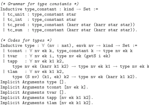
(* Grammar for type constants *)

Inductive type_constant : kind → Set := | tc_unit : type_constant star

| tc_int : type_constant star

| tc_prod : type_constant (karr star (karr star star)) | tc_sum : type_constant (karr star (karr star star)).

(* Codes for types *)

Inductive type : ∀ (nv : nat), envk nv → kind → Set := | tconst : ∀ nv ek k, type_constant k → type nv ek k | tvar : ∀ nv ek i, type nv ek (getS i ek)

| tapp : ∀ nv ek k1 k2,

type nv ek (karr k1 k2) → type nv ek k1 → type nv ek k2 | tlam : ∀ nv ek k1 k2,

type (S nv) (k1, ek) k2 → type nv ek (karr k1 k2). Implicit Arguments type [].

Implicit Arguments tconst [nv ek k]. Implicit Arguments tvar [].

Implicit Arguments tapp [nv ek k1 k2]. Implicit Arguments tlam [nv ek k1 k2].

(* Syntactic sugar for types with no free variables *)

Definition closed_type (k : kind) : Set := type 0 tt k.

(* Syntactic sugar for type constants *)

Definition tunit := tconst 0 tt tc_unit. Definition tint := tconst 0 tt tc_int. Definition tprod := tconst 0 tt tc_prod. Definition tsum := tconst 0 tt tc_sum

Fig. 2. Generic view.

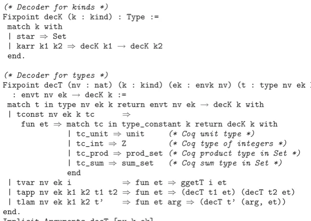
Similarly, we need to encode kinds and provide the associated decoder. The codes for types and kinds are often called a generic view or a universe. The definitions for our generic view are given in Figure 2, and the decoders for kinds and types are defined in Figure 3. Our universe for types encodes only well-kinded types; this is explained in Section 3.1. The decoders for kinds and types are discussed in Sections 3.2 and 3.3, and we conclude with a few examples in Section 3.4.

3.1 Kinding derivations

In our definition of the generic view, we do not define a datatype that encodes the grammar of types, but rather encode kinding derivations to make sure that only well-kinded types can be represented. An element

(* Decoder for kinds *)

Fixpoint decK (k : kind) : Type := match k with

| star ⇒ Set

| karr k1 k2 ⇒ decK k1 → decK k2 end.

(* Decoder for types *)

Fixpoint decT (nv : nat) (k : kind) (ek : envk nv) (t : type nv ek k) : envt nv ek → decK k :=

match t in type nv ek k return envt nv ek → decK k with | tconst nv ek k tc ⇒

fun et ⇒ match tc in type_constant k return decK k with | tc_unit ⇒ unit (* Coq unit type *)

| tc_int ⇒ Z (* Coq type of integers *)

| tc_prod ⇒ prod_set (* Coq product type in Set *)

| tc_sum ⇒ sum_set (* Coq sum type in Set *)

end

| tvar nv ek i ⇒ fun et ⇒ ggetT i et

| tapp nv ek k1 k2 t1 t2 ⇒ fun et ⇒ (decT t1 et) (decT t2 et) | tlam nv ek k1 k2 t’ ⇒ fun et arg ⇒ (decT t’ (arg, et)) end.

Implicit Arguments decT [nv k ek].

Fig. 3. Decoders.

is a type of kind k with at most nv free variables, whose kinds are defined in the kind environmentek. This corresponds to a kinding derivation

ekT :k

The type of the environment ek is envk nv, which is an nv-tuple of kinds (see Figure 2). As an example, the ruletlamfor lambda abstraction encodes the kinding derivation

(k1, ek)T :k2 ekΛT :k1 →k2

Lam

We use de Bruijn indices to represent variables (de Bruijn 1972). The indices in a type of nv free variables cannot be out of bounds since their type is index nv (Section 2.4).

3.2 Decoding kinds

The decoderdecKfor kinds is straightforward except for a subtlety in the choice of

Setfor kind. During type specialization (Section 5), we will construct types of the form

(∀(α:decK star), . . .) :decK star

so that using Type for (decK star) will result in a universe inconsistency. Hence, we choose Setinstead, enabling the impredicativeSetoption1.

Another way to solve the impredicativity problem is to stratify kinds themselves, i.e. to assign different levels to kind depending on nesting depth. We would then get something of the form

(∀(α:decK stari). . . .) :decK starj

Here it is possible to use Type as the decoding of kind , with different universe levels assigned to the different nesting levels of the kinds. We have opted to use impredicativeSetinstead, because we did not want to complicate the kind universe. It would be interesting to see how the infrastructure would change if we used stratified kinds.

3.3 Decoding types

The decoder decT for types is more involved. To decode a type T with nv free variables, we must know the decoded types of the free variables in T. Hence, we need an environment etof type envt that associates a decoded typeTi with every

free variable i in T. Since the kind of Ti depends on the kind ofi, each element in

ethas a different type. We therefore calculateenvtfrom the kind environment ek:

Definition envt nv (ek : envk nv) := gtupleT decK ek

using the heterogeneous tuple gtupleTdescribed in Section 2.6.

Armed with the type environment et we define the decoder for types decT as shown in Figure 3. Type constants map to their Coq counterparts, variables map to the corresponding elements in the environmentet, application maps to Coq type application and lambda abstraction maps to Coq type-level functions. To decode the body of a lambda abstraction, we must add the type of the formal parameter to the type environment.

3.4 Example types

In this section we will consider some examples of types, defined as codes in our generic view with the associated decoding. We have added some notational shorthand to make these example types more readable:

Notation "t @ s" := (tapp t s) (at level 30).

Notation "t + s" := (tapp (tapp (tconst tc_sum) t) s). Notation "t × s" := (tapp (tapp (tconst tc_prod) t) s). Notation "1" := (tconst tc_unit).

Unfortunately, the definitions are still a little heavy on notation, especially in dealing with type variables – var i represents the ith variable – but additional syntactic sugar is left to future work.

Consider the typefork, defined in Haskell as

data Fork a = MkFork a a

We encode this as a type with one argument ΛA . A×A in our generic view as

Definition fork : closed_type (karr star star) := let var := tvar 1 (star, tt)

in tlam (var None × var None).

The type of fork tells us that it is a closed type of kind → . We decode fork

to a Coq type using our type decoder decT, where tt represents the empty type environment:

Eval compute in decT fork tt.

= (fun A : Set ⇒ A × A) : decK (karr star star)

The command Eval r in x performs the reductions specified byr on the term x

and displays the resulting term with its type. In this case we use the tacticcompute to specify the reductions, which represents call-by-valueβ,δ,ιandζ-reduction.

We can evaluate the decoding of the kind→of fork using the kind decoder

decKin a similar fashion:

Eval compute in decK (karr star star).

= (Set → Set) : Type

As another example, consider the typemaybe prod, defined in Haskell as

data MaybeProd a b = NoProd | SomeProd a b

This type has kind→→. We encode it as a type ΛA .ΛB .1 +A×B as

Definition maybe_prod

: closed_type (karr star (karr star star)) := let var := tvar 2 (star, (star, tt)) in

tlam (tlam (1 + (var (Some None) × var None))).

Decoding the typemaybe prodgives

Eval compute in decT maybe_prod tt.

= fun A B : Set ⇒ unit + A × B

which gives us a Coq function in two arguments of type Set. Note that unit is the predefined unit type in Coq, and×and + are the predefined product and sum types.

Finally, we show the code forapply : (→)→→. Its Haskell counterpart is

It takes a type constructorF:→and a typeA:and applies FtoA:

Definition apply

: closed_type (karr (karr star star) (karr star star)) := let var := tvar 2 (star, (karr star star, tt)) in

tlam (tlam (var (Some None) @ var None)).

The decoding will again be an actual Coq function:

Eval compute in decT apply tt.

= fun (F : Set → Set) (A : Set) ⇒ F A

4 Defining polytypic functions

In this section, we show how to define polytypic types (Section 4.1) and polytypic functions (Section 4.2) in our framework, and give a number of examples (Sec-tions 4.3 and 4.4). Polytypic func(Sec-tions are defined by giving instances for the type constants in the universe, which we stated in Section 3. We hope that readers familiar with Generic Haskell or Generic Clean will experience a comforting familiarity reading our definitions; we will explain specifics pertaining to Coq as they arise. We will discuss type and term specialization but we will not formalize these concepts until Sections 5 and 6 respectively.

4.1 Polytypic types

The type of a polytypic function is a type-level function which, givennparguments, constructs a type of kind . This is represented by the following record:

Record PolyType (np : nat) : Type := polyType { typeKindStar : nary_fn np (decK star) (decK star) }.

Record introduces a record of named fields. PolyType depends on one parameter (np) and has one field (typeKindStar) of type nary fn np (decK star) (decK star). The termnary fnn A B denotes the type

A→. . .→A

n

→B

Argument np, known as the arity of the polytypic function in Generic Haskell, represents the number of type arguments – it does not refer to the number of arguments of the specialized function, which varies with the kind of the target type. Readers familiar with polytypic programming will know that map is a polytypic function of arity 2; its type is

Definition Map : PolyType 2 := polyType 2 (fun A B ⇒ A → B).

In Generic Haskell we would give the typeMapasA→B; whereas in Coq we have to explicitly state the type argumentsAandB. Note also that the record constructor

of type argumentsnpas well as the fieldtypeKindStar. The type of the polytypic function describes the operation performed at the elements:maptransforms elements of typeAto elements of typeB. Term specialization lifts this operation to structures containing elements and type specialization gives the type of the lifted operation. Informally, type specialization is described as

Ptk : k→ · · · →k→

PtT1. . . Tnp = (user defined)

Ptk1→k2T1. . . Tnp = ∀A1. . . Anp .Ptk1A1. . . Anp →Ptk2(T1A1) . . .(Tnp Anp).

This is formalized as a functionspecType(defined in Section 5), so that we can ask Coq to specialize a polytypic type for us. For example, here is the specialization of

Map→→applied to two copies of the product type:

Eval compute in specType tprod Map.

= ∀ A B : Set, (A → B) →

∀ C D : Set, (C → D) → A × C → B × D

4.2 Polytypic functions

To define a polytypic function, the user only needs to provide the definition for the type constants; term specialization takes care of the remaining types. A nice feature of an implementation of polytypic programming in a dependently typed language is that a polytypic function is simply another record which can be passed as an argument to, or computed as the result of, a function.

We define a polytypic function as

Record PolyFn (np : nat) (Pt : PolyType np) : Type := polyFn { punit : specType tunit Pt ;

pint : specType tint Pt ;

pprod : specType tprod Pt ;

psum : specType tsum Pt

}.

Implicit Arguments PolyFn [np].

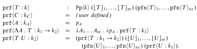
A polytypic function of np arguments has a polytypic type Pt of np arguments and provides definitions for each of the type constants. The types of these fields are computed by type specialization, ensuring that ill-typed polytypic functions cannot be defined. Moreover, as we have seen, we can ask Coq to evaluate these types, which helps guide us in the construction of a polytypic function. Term specialization is then informally described as

pfnT :k : Ptk(T1, . . . ,Tnp)

pfnC:kC = (user defined)

pfnA:kA = fA

pfnΛA . T :k1→k2 = λA1. . . Anp . λfA .pfnT :k2

where Ti replaces each free variable A in T by Ai. This definition of pfn is

formalized as a functionspecTerm(Section 6). For example, specializingmap(defined in Figure 1) to the datatype forkof kind→yields

Eval compute in specTerm fork map.

= fun (A B : Set) (f : A → B) (x : A × A) ⇒

let (a1, a2) := x in (f a1, f a2) : specType fork Map

Term specialization returns an actual Coq function, which can be applied to further arguments:

Eval compute in specTerm fork map nat nat (fun x ⇒ x + 1) (3, 5).

= (4, 6)

4.3 Examples of polytypic types and functions

As a first example, we will consider the polytypic functioncount, which counts the elements in a data structure:

Definition Count : PolyType 1 :=

polyType 1 (fun A ⇒ A → nat).

Definition count : PolyFn Count := polyFn Count

(fun u ⇒ 0)

(fun z ⇒ 0)

(fun (A : Set) (f : A → nat)

(B : Set) (g : B → nat)

(x : A × B) ⇒

let (a, b) := x in (plus (f a) (g b)))

(fun (A : Set) (f : A → nat)

(B : Set) (g : B → nat)

(x : A + B) ⇒

match x with

| inl a ⇒ f a

| inr b ⇒ g b

end).

Types of kind never contain any elements, so we simply return 0 when counting units or integers. For other types, we pass in a function that converts each element into a natural number, and count adds these all up. For example, to count the number of elements in a list we could pass in the constant function that takes each element to the number 1; adding these all upcountwould give us the length of the list. We specialize both Countandcountto the datatypefork:

Eval compute in specType fork Count.

Definition equal : PolyFn Compare := polyFn Compare

(fun x y ⇒ true)

Zeq_bool

(fun (A : Set) (f : A → A → bool)

(B : Set) (g : B→ B → bool)

(x : A × B) (y : A × B) ⇒

let (a , b ) := x in let (a’, b’) := y in

f a a’ && g b b’)

(fun (A : Set) (f : A → A → bool)

(B : Set) (g : B→ B → bool)

(x : A + B) (y : A + B)⇒

match (x, y) with

| (inl a, inl a’) ⇒ f a a’

| (inr b, inr b’) ⇒ g b b’

| otherwise ⇒ false

end).

Definition less_than : PolyFn Compare := polyFn Compare

(fun x y ⇒ false)

(fun x y ⇒ Zlt_bool x y)

(fun (A : Set) (f : A → A → bool)

(B : Set) (g : B → B → bool)

(x : A × B) (y : A × B) ⇒

let (a, b) := x in let (a’, b’) := y in

f a a’ && g b b’)

(fun (A : Set) (f : A → A → bool)

(B : Set) (g : B → B → bool)

(x : A + B) (y : A + B) ⇒

match (x, y) with

| (inl a, inl a’) ⇒ f a a’

| (inr b, inr b’) ⇒ g b b’

| otherwise ⇒ false

end).

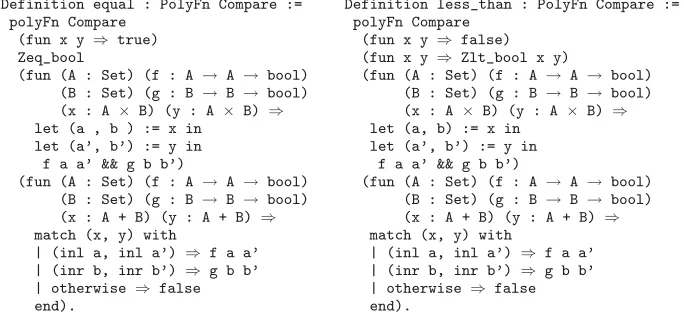
Fig. 4. Polytypic functionsequalandless than.

Eval compute in specTerm fork count.

= fun (A : Set) (f : A → nat) (x : A × A) ⇒

let (a, a’) := x in f a + f a’.

As two further examples, considerequalandless than. These functions compare their arguments for equality or check that the first is less than the second. The function less than can be thought of as “pair-wise comparison” or “coordinate-wise order”. Lexicographical ordering would perhaps be more sensible on arbitrary data structures, but is a more involved example. We use pair-wise comparison instead to avoid getting bogged down in the details of the example. These two comparison functions are quite similar and even share the same polytypic typeCompare:

Definition Compare : PolyType 1 :=

polyType 1 (fun A ⇒ A → A → bool),

which, specialized tofork, yields

Eval compute in specType fork Compare.

= ∀ A : Set, (A → A → bool) → A × A → A × A → bool.

Since bothless than andequal will return false when their arguments have a different structure, the definitions of these two polytypic functions are also quite similar. The only difference is how they compare elements of unit or integer type. The definitions of these two polytypic functions can be found in Figure 4.

In Section 7.4 we will show that even though less than and equal are very similar, they do have different properties: we will prove that equality is commutative butless thanis anti-commutative.

4.4 First-class polytypic functions

and be computed as results. As an example of such apolytypic combinator, we define “or poly”, which computes the “disjunction” of two other polytypic functions of type Compare:

Definition or_poly (pfn1 pfn2 : PolyFn Compare) : PolyFn Compare :=

polyFn Compare

(fun u v ⇒ punit pfn1 u v || punit pfn2 u v)

(fun i j ⇒ pint pfn1 i j || pint pfn2 i j)

(fun (A : Set) (f : A → A → bool)

(B : Set) (g : B → B → bool)

(x y : A × B),

pprod pfn1 A f B g x y || pprod pfn2 A f B g x y)

(fun (A : Set) (f : A → A → bool)

(B : Set) (g : B → B → bool)

(x y : A + B),

psum pfn1 A f B g x y || psum pfn2 A f B g x y).

Less-than-or-equal-to can now be defined by applying this combinator to the two polytypic functionsequalandless than we defined above:

Definition le : PolyFn Compare := or_poly equal less_than.

When we specialize the polytypic functionleto the typeT= ΛA .ΛB . A+Z×B, we get a function which is provably equal to

fun (A : Set) (f : A → A → bool) (B : Set) (g : B → B → bool)

(x y : decT T tt A B) ⇒

match (x, y) with

| (inl a, inl a’) ⇒ f a a’

| (inr (z, b), inr (z’, b’)) ⇒ Zle_bool z z’ && g b b’

| _ ⇒ false

end

The proof that these two are equal can be found in first class.v in the Coq sources. Although it is not clear how many higher-order polytypic functions we will be able to define in this fashion, if a function can be so defined then the infrastructure for proofs we provide in this paper is immediately applicable, which can be very helpful. For instance, although le can be defined in Generic Haskell (or indeed using our library) by conjoining the instances of equal and less than

(leT = equalT || less thanT), this does not have the right shape for our proof framework so that the support for polytypic proofs is not available. A further discussion of first-class polytypic functions falls outside the scope of this paper.

5 Type specialization

(* Environment of the form ((a_1, b_1, ..), .., (a_np, b_np, ..)) to keep track of free variable replacements

in type and term specialization *)

Definition envts (np nv : nat) (ek : envk nv) := tupleT (envt nv ek) np.

(* Specialize polytypic type Pt to kind k *)

Fixpoint kit (k : kind) (np : nat) (Pt : PolyType np) : tupleT (decK k) np → decK star :=

match k return tupleT (decK k) np → decK star with | star ⇒ uncurry (typeKindStar Pt)

| karr k1 k2 ⇒ fun tup ⇒ quantify_tuple

(fun As ⇒ kit k1 Pt As → kit k2 Pt (apply_tupleT tup As)) end.

Implicit Arguments kit [np].

(* Type specialization for open types *)

Definition specType’ (np nv : nat) (k : kind) (ek : envk nv) (t : type nv ek k) (Pt : PolyType np) (ets : envts np nv ek) : decK star :=

kit k Pt (replace_fvs t ets).

Implicit Arguments specType’ [np nv k ek].

(* Type specialization for closed types *)

Definition specType (np : nat) (k : kind) (t : closed_type k) (Pt : PolyType np) : decK star :=

specType’ t Pt (ets_tt np). Implicit Arguments specType [np k].

Fig. 5. Type specialization.

how to define type specialization. The full definition of type specialization is given in Figure 5. This and the next section are technical sections, which can be skipped by readers who are interested only in theapplication of our infrastructure.

Type specialization is a two-phase process. We first define the kind-indexed type

kit, where kit k Map corresponds to Ptk in the informal definition given in Section 4.1, by induction onk. We then apply the result to the appropriate tuple of type arguments.

The case for kindis supplied by the user (PolyType, see Section 4). We rewrite the case for arrow kinds as

Ptk1→k2= ΛT1. . . Tnp .∀A1. . . Anp .(. . .)

to make it more obvious that we must return a type-level function which, givennp arguments, returns a universally quantified type. To give a recursive definition of this type, a simple but helpful insight is that it is easier to work with an uncurried form (Altenkirch & McBride 2003):

Λ(T1, . . . , Tnp).∀A1. . . Anp .Ptk1(A1, . . . , Anp)→Ptk2(T1A1, . . . , Tnp Anp).

To construct this function, we first construct the function where both theT’s and

A’s are uncurried:

Λ(T1, . . . , Tnp).Λ(A1, . . . , Anp).Ptk1(A1, . . . , Anp)→Ptk2(T1 A1, . . . , Tnp Anp)

This definition can be translated to the correct type using the functionquantify tuple(defined intuples.vin the Coq sources), which takes a function of the form

Λ(A1, . . . , Anp). T

to the universally quantified type

∀A1. . . Anp . T .

Paraphrasing, kit k Ptconstructs a type that calculates the required specialized type given a tuple (T1, . . . , Tnp); the second step in type specialization is therefore to

construct this tuple. Hinze (2000) states that specialization of a polytypic function

pfnof typePtto a typeT has type

pfnT :k:Ptk(T1, . . . ,Tnp).

The floor operatorTireplaces all free variablesAinT byAi. For a closed typeT

this will have no effect as there are no free variables to replace. To explain this in more detail, let us consider an example: the typeMapspecialized toT = ΛA B C . A+B×C

should be

(A1→A2)→(B1→B2)→(C1→C2)→T A1B1 C1→T A2B2C2

Recall that the polytypic type Map, which describes the type of the operations map

performs at the elements of a structure, is ΛA1 A2 . A1 →A2. When we specialize

mapto a specific datatype, we will need an instance of this operation for each of the arguments of that datatype. Hence, if the datatype has nv parameters, we will need nv copies of this operation, each of which will need np type arguments. To keep track of all of these types, we construct an environmentets:envts of the form

((A1, B1, . . .),(A2, B2, . . .), . . . ,(Anp, Bnp, . . .))

The floor operation Ti replaces each free variable in T (each argument of the

datatype) by the ith variable associated with it by extracting the ith tuple from the environment and then decoding T using this tuple as the type environment (Section 3.3).

Returning to our example, for every ΛA . · · · we encounter during term special-ization we will add the elements of the tuple (A1, . . . , Anp) to the front of the tuples

already in ets(Section 6.4), using a function add to ets to accomplish this. The type of the specialization of thebody of the lambda abstractions inT will then be

Ptk(A+B×C1, . . . ,A+B×Cnp)

When we specialize a function to a closed type (nv = 0),etsis the tuple containing np empty tuples – constructed by ets tt np – and (T1, . . . ,Tnp) reduces to

The full definition of type specialization is given in Figure 5. The function kit

constructs kind-indexed types and specType’ returns the application of a kind-indexed type to a tuple (T1, . . . ,Tnp). This tuple of types is constructed by

replace fvs, whose definition is straightforward and can be found in the Coq sources.

6 Term specialization

Having seen how to define polytypic functions in Section 4 and how to specialize their types in Section 5, we are now in a position to define term specialization. Since the result of term specialization has a specialized type, our implementation is a formalproof that the result of term specialization is a term of the type computed by type specialization. The subsections in this section correspond to each of the type constructors for constants, variables, type application and type abstraction.

A polytypic function is fully specified by giving its type and the cases for each of the type constants. The cases for the other types can be inferred; an informal definition of this process pfnT :kwas given in Section 4.2. In this section, we discuss its formalization in Coq. The type of term specialization is

specTerm : ∀ (np : nat) (k : kind) (t : closed_type k)

(Pt : PolyType np) (pfn : PolyFn Pt), specType t Pt

The definition is shown in Figure 6; it relies on a number of auxiliary lemmas which we do not show but will explain below (the full definitions can be found in the Coq sources).

6.1 Constants

For type constants we have to use the definition provided by the user, but there is a mismatch in the type of the term provided by the user and the return type of term specialization. Consider the case for the product constant. As part of the definition of the polytypic function, the user will have provided a functionpprodof type

pprod : specType tprod Pt

Recall from Figure 2 thattprod is syntactic sugar for

tconst 0 tt tc_prod

As described in Section 3, terms of type type encode kinding derivations; tprod

encodes the derivation in the empty environmenttt

∅ tconst tc prod:→→ Const

When tc prod is used inside another type; however, it may well be used in an environment where thereare free variables.2 _{This arises, for instance, in the use of}

(* Specialize the polytypic function pfn to open type t *)

Fixpoint specTerm’ (np nv : nat) (ek : envk nv) (k : kind) (t : type nv ek k) (Pt : PolyType np) (pfn : PolyFn Pt) : ∀ (ets : envts np nv ek) (ef : envf nv ek Pt ets),

specType’ t Pt ets := match t in type nv ek k

return ∀ (ets : envts np nv ek),

envf nv ek Pt ets → specType’ t Pt ets with

| tconst nv ek k tc ⇒ fun ets ef ⇒

match tc return specType’ (tconst tc) Pt ets with

| tc_unit ⇒ convertS convert_tconst_specTerm (punit pfn) | tc_int ⇒ convertS convert_tconst_specTerm (pint pfn) | tc_prod ⇒ convertS convert_tconst_specTerm (pprod pfn) | tc_sum ⇒ convertS convert_tconst_specTerm (psum pfn) end

| tvar nv ek i ⇒ fun ets ef ⇒ convertT ith_index_f (ggetS i ef) | tapp nv ek k1 k2 t1 t2 ⇒ fun ets ef ⇒

convertS convert_tapp_specTerm

((instantiate_tuple (replace_fvs t2 ets)

(specTerm’ t1 pfn ets ef)) (specTerm’ t2 pfn ets ef)) | tlam nv ek k1 k2 t’ ⇒

fun ets ef ⇒ dep_curry (fun As ⇒ kit k1 Pt As →

kit k2 Pt

(apply_tupleT (replace_fvs (tlam t’) ets) As)) (fun As : tupleT (decK k1) np ⇒

(fun fa : kit k1 Pt As ⇒

(convertS (convert_tlam_specTerm _ _ _ _)

(specTerm’ t’ pfn (add_to_ets As ets) (add_to_ef fa ef))))) end.

Implicit Arguments specTerm’ [np nv ek k Pt].

(* Term specialization for closed types *)

Definition specTerm (np : nat) (k : kind) (t : closed_type k) (Pt : PolyType np) (pfn : PolyFn Pt) : specType t Pt := specTerm’ t pfn (ets_tt np) tt.

Implicit Arguments specTerm [np k Pt].

Fig. 6. Term specialization.

tc prodin the definition offorkin Section 3.4, where instead we have a derivation of the form

A:tconst tc prod:→→ Const

In general, we need the type encoding

tconst nv ek tc_prod

for a number of free variables nvand the associated kind environmentek.

We could generalize the definition of the polytypic function given in Section 4.2 to

Record PolyFn (np : nat) (Pt : PolyType np) : Type := polyFn { ...

specType’ (tconst nv ek tc_prod) Pt ets ; ...

}.

However, this generalization complicates both the definition of a polytypic function and the instances the user must provide. Fortunately, it turns out that a polytypic type specialized to tconst nv ek tc prod is the same as that type specialized to

tconst 0 tt tc prod, as proved by the following weakening lemma.

Lemma 2(convert tconst specTerm)

∀ nv ek tc Pt ets,

specType (tconst 0 tt tc) Pt = specType’ (tconst nv ek tc) Pt ets

Proof. Unfolding definitions (Figure 5), we find that we have to prove

(tconst 0 tt tc1, . . .) = (tconst nv ek tc1, . . .)

This holds as decoding a type constant is independent of the environment

provided.

6.2 Variables

Recall from the informal definition of term specialization (Section 4.2) that in the case for variables we return the function fA constructed in the clause for lambda

abstraction; in the formalization we will use an environment ef containing the appropriate function for each free variable. The interesting part is to assign a type

envf to ef, since each element in ef has a different type. We define envf as a heterogeneous tuple (Section 2.6).

Definition envf np nv ek Pt ets :=

gtupleS (fun i ⇒ specType’ (tvar nv ek i) Pt ets)

(elements_of_index nv)

The type of theith function is the specialized type of the ith free variable. Thus, we map specType’ across the tuple containing all possible indices of type index nvconstructed byelements of index. Given ef, we simply return theith element in efas the specialized term for variable i. However, due to the way we calculate

envfwe do need one technical lemma in the case for variables:ith index fstates that applying a functionf to theith element ofelements of index is the same as applyingf toi, which results in a proof that theith element will always be the index

6.3 Application

To specialize a polytypic function pfn of type Pt to a type application (T U), we first specialize toT:k1→k2, which will create a term of the form

specTerm’ T pfn ets ef :

∀A1. . .Anp, kit k1 Pt(A1, . . . ,Anp)→kit k2 Pt(T1A1, . . . ,Tnp Anp)

We instantiate the type variablesA1. . .Anp to the elements of the tuple (U1, . . . ,Unp)

using the following function:

instantiate_tuple (A : Type) (n : nat) :

∀ (args : tupleT A n) (X : tupleT A n → Set),

quantify_tuple X → X args

(see Coq source for a full definition). This leaves us with the following term:

(specTerm’ T pfn ets ef)U1. . .Unp

: kit k1 Pt(U1, . . . ,Unp)→kit k2 Pt(T1U1, . . . ,Tnp Unp)

We apply this term to the polytypic function specialized to the type U, which serendipitously has exactly the right type, and get a term of type

kit k2 Pt(T1U1, . . . ,Tnp Unp).

Since we are specializing to the application (T U), the return type we expect here is

specType’ (tapp T U) Pt ets.

We then use the following lemma to complete the definition for application.

Lemma 3 (convert tapp specTerm)

∀np k1 k2 Pt ets(T:k1→k2) (U:k1),

kit k2 Pt(T1U1, . . . ,Tnp Unp) =specType’ (tapp T U) Pt ets

Unfolding definitions (Figure 5), we find that we have to prove that

(T1 U1, . . . ,Tnp Unp) = (T U1, . . . ,T Unp)

This holds as replacing free variables before or after application gives the same

result.

6.4 Lambda abstraction

In this section, we will look at the specialization of a polytypic functionpfnof type

Ptto a lambda abstraction (ΛA.T). The type of this specialization must be

specTerm’ (tlam T) pfn ets ef:specType’ (tlam T) Pt ets

which can be unfolded to

∀A1. . .Anp, kit k1 Pt(tlam T1, . . . ,tlam Tnp)→

We will construct this term in two steps. We use the specialization of pfn to T

to construct the body of the expression and use currying to get arguments of the correct type.

6.4.1 Dependent currying

We will construct the required term by first defining a function of the form

fun(A1, . . . ,Anp)fA⇒. . .

which we then curry to get

fun A1. . .Anp fA⇒. . .

We cannot use the standard definition of currying, however. The type of the body is

kit k2 Pt(tlam T1A1, . . . ,tlam Tnp Anp)

and depends on the actual argument tuple that is supplied. We therefore need a dependent curry function, which can be defined as

Fixpoint dep_curry (A : Type) (n : nat)

: ∀ (C : tupleT A n → Set) (f : ∀ (x : tupleT A n), C x),

quantify_tuple C :=

match n return ∀ (C : tupleT A n → Set)

(f : ∀ (x : tupleT A n), C x), quantify_tuple C

with

| O ⇒ fun _ f ⇒ f tt

| S m ⇒ fun c f a ⇒

dep_curry A m (fun args ⇒ c (a, args))

(fun args ⇒ f (a, args))

end.

Implicit Arguments dep_curry [A n].

6.4.2 Specialization toT

To construct the body of the result, we use the specialization of pfntoT:

specTerm’ T pfn(add to ets(A1, . . . ,Anp)ets)(add to ef fA ef)

:specType’ T Pt(add to ets(A1, . . . ,Anp)ets)

This term does not have the correct type, so we need the following conversion lemma.

Lemma 4(convert tlam specTerm)

∀k2 T Pt ets(A1, . . . ,Anp),

specType’ T Pt(add to ets(A1, . . . ,Anp)ets)

Unfolding definitions (Figure 5), we find that we have to prove that

(T1, . . . ,Tnp) using (add to ets(A1, . . . ,Anp)ets)

= (tlam T1 A1, . . . ,tlam Tnp Anp) usingets

This holds as decoding a lambda abstraction and applying it to A is the same as decoding the body of the lambda abstraction withAadded to the front of the type

environment.

6.4.3 AddingfA to the function environment

The current environment ef has an entry for each free variable in tlam T, but variable i in tlam T becomes variable Somei (i+ 1) in the bodyT. Therefore, the function fX associated with theith variableX in the old environment

fX :specType’ (tvar nv ek i) Pt ets

should have type

fX :specType’ (tvar (S nv) (k1, ek) (Some i)) Pt

(add to ets(A1, . . . ,Anp)ets)

in the new environment. The following lemma proves that these two types are equal.

Lemma 5 (convert envf)

∀nv ek k1 i Pt ets (A1, . . . ,Anp),

specType’ (tvar nv ek i) Pt ets

=specType’ (tvar (S nv) (k1, ek) (Some i)) Pt

(add to ets (A1, . . . ,Anp) ets)

Proof. Unfolding definitions (Figure 5), we find that we have to prove

(tvar nv ek i1, . . .) usingets

= (tvar (S nv) (k1, ek) (Some i)1, . . .) using (add to ets(A1, . . . ,Anp)ets).

To decode variableiwe take theith element from the environment, which is the same as taking the elementSomeifrom an environment containing one extra element. When the type of every function in efhas been shifted in this way, we can add the argument to the lambda abstraction fA to the start of ef. We need one more

lemma.

Lemma 6 (convert envf elem)

∀nv ek k1 Pt ets (A1, . . . ,Anp),

kit k1 Pt (A1, . . . ,Anp) =kit k1 Pt (tvar (S nv) (k1, ek) None1, . . .)

It suffices to prove

(A1, . . . ,Anp)

= (tvar (S nv) (k1, ek) None1, . . .) using (add to ets(A1, . . . ,Anp)ets).

7 Polytypic Properties and Proofs

In Sections 3–6 we discussed the infrastructure needed for specializing polytypic types and polytypic functions. We now turn toproofs over polytypic functions. We discuss how properties of polytypic functions can be stated (Sections 7.1 and 7.2), what polytypic proofs will look like (Section 7.3) and give a few examples (Section 7.4). We conclude with a discussion of alternative formalizations of polytypic properties (Section 7.5); this can be skipped if desired. The formalization of property and proof specialization will be the topic of Sections 8 and 9.

As an introductory example, we will see how to prove that map preserves identity and composition. These two laws are known as the “functor laws”, in reference to the laws that a functor must satisfy in category theory. In the case of a unary type constructor, such asfork :→ (Section 3.4), the functor laws formap take the form:

mapforkid = id

mapfork(f◦g) = mapforkf◦mapforkg.

However, given a type constructor of two arguments such asmaybe prod:→→, the functor laws take a different shape:

mapmaybe prodid id = id

mapmaybe prod(f◦g) (h◦k) = mapmaybe prodf h◦mapmaybe prodg k.

The shape of these properties therefore depends on the kind of the datatype we specialize to. Fortunately, we can state and prove such properties in much the same way as we type and define polytypic functions.

We have seen how we can formally interpret the informal notationpfnTfor the specialization of a polytypic functionpfn to a datatype T and the notationPtk

for the specialization of a polytypic typePt to a kindk. To aid readability, we will now feel free to switch back to the informal notation and trust that the reader will understand the interpretation of the informal notation as explained previously.

7.1 Stating polytypic properties

To specify a polytypic property we have to give the types of the functions that the property ranges over and the property itself. Take the example that map preserves identity: this property ranges over functions of typeMap; sinceMapis kind-indexed, it follows that the property itself is kind-indexed:

IdkT :MapkT T →Prop.

In the case for kind, the typeMapT T specializes to the function typeT →T

and the corresponding property is that the function must itself be the identity function:

IdT : (T →T)→Prop

IdT = λf:T →T .∀x:T . f x=x.