Small area estimation: new developments and directions

Small Area Estimation – New Developments and Directions

Danny Pfeffermann

appears in International Statistical Review, 2002

Department of Statistics, Hebrew University, Jerusalem, Israel

Department of Social Statistics, University of Southampton, United Kingdom

Summary

The purpose of this paper is to provide a critical review of the main advances in small area estimation (SAE) methods in recent years. We also discuss some of the earlier developments, which serve as a necessary background for the new studies. The review focuses on model dependent methods with special emphasis on point prediction of the target area quantities, and mean square error assessments. The new models considered are models used for discrete measurements, time series models and models that arise under informative sampling. The possible gains from modeling the correlations among small area random effects used to represent the unexplained variation of the small area target quantities are examined. For review and appraisal of the earlier methods used for SAE, see Ghosh and Rao (1994).

Key words:

1 Introduction

The problem of SAE is twofold. First is the fundamental question of how to produce reliable estimates of characteristics of interest, (means, counts, quantiles, etc.) for small areas or domains, based on very small samples taken from these areas. The second related question is how to assess the estimation error. Note in this respect that except in rare cases, sampling designs and in particular sample sizes are chosen in practice so as to provide reliable estimates for aggregates of the small areas such as large geographical regions or broad demographic groups. Budget and other constraints usually prevent the allocation of sufficiently large samples to each of the small areas. Also, it is often the case that domains of interest are only specified after the survey has already been designed and carried out. Having only a small sample (and possibly an empty sample) in a given area, the only possible solution to the estimation problem is to borrow information from other related data sets. Potential data sources can be divided into two broad categories:

Data measured for the characteristics of interest in other ‘similar’ areas, Data measured for the characteristics of interest on previous occasions.

The methods used for SAE can be divided accordingly by the related data sources that they employ, whether cross-sectional (from other areas), past data or both. A further division classifies the methods by the type of inference: ‘design based’, ‘model dependent’ (with sub-division into the frequentist and Bayesian approaches), or the combination of the two. In what follows I describe briefly two real applications of SAE that illustrate what the areas or domains might be, the quantities of interest and the kind of concomitant variables that are used for estimation. Other examples are mentioned in subsequent sections.

coefficients and state and sub-state random effects with age group specific elements as the independent variables (see Section 4.) The regressor variables comprise person and block group level demographic variables, census tract level demographic and socio-economic status variables and county level rates of drug-related arrests and deaths. The auxiliary information is available from various administrate records. For a detailed description of the NHSDA and the other data sources, the modeling process and estimates released, see the web site:

http://www.samhsa.gov/oas/NHSDA/1999/Table%20of%20Contents.htm. The article by Folsom et al. (1999) expands on methodological issues.

B-

Estimation of Small Area Employment

employment in CES sample + non-sample predicted employment + “add-ons”.

domain ES202 benchmark employment for non-sample businesses and Rˆ is the ratio

adjust for employment that cannot be assigned to the industry division through specific firms. Enhancements to the above small domain estimates are currently investigated.

The purpose of this paper is to discuss some of the recent developments in SAE. The main emphasis is on general methodological issues rather than on detailed technical solutions. For these, as well as some recent applications of SAE, the reader is referred to the new review article by Rao (1999), which is an update of the more extensive review of Ghosh and Rao (1994). Another recent review of SAE methods is the article by Marker (1999).

Section 2 illustrates the important role of administrative information for SAE and introduces the family of synthetic regression estimators. Section 3 reviews several cross-sectional models in common use for continuous measurements. These models are extended to handle discrete measurements in Section 4 and to account for time series relationships in Section 5. The analysis in Sections 3-5 assumes implicitly that the sampling process can be ignored for inference. Section 6 considers the case of informative sampling under which the sample data no longer represent the population model. Section 7 examines the importance of modeling the correlations among the random area effects. I conclude with brief remarks in Section 8.

2 The importance of concomitant administrative data, synthetic estimation

In this and the next three sections we assume for convenience that the sample is selected by simple random sampling without replacement. The possible implications of the use of complex sampling schemes with unequal selection probabilities are discussed in Section 6. Let y define the characteristic of interest and denote by y_ij the outcome value for unit j belonging to area i, i 1...m; j 1...Ni, where Ni is the area size. Let s s1‰...‰sm signify the sample where s_i of size n_i defines the sample observed for area i. Notice that the

s

n_i’ are random unless a separate sample with fixed sample size is taken in every area. Suppose that the objective is to estimate the true area mean

¦

i N

j ij i

i y N

i n

j ij

i y n

y i / 1

¦

( ] |

[ i i i i i i i

D y n S n n N S

V (2.1)

where ¦

i i

N

j yij Yi Ni

S2 1( )2/( 1)

~ _{. Clearly, for small}

i

n the variance will be large unless the variability of the y-values is sufficiently small. Suppose, however, that in addition to measuring y, values x_ij of p concomitant variables x(1)...x(p) are also known for each of the sample units and that the row area means Ni₁ /

i j ij i

X

¦

( )’ ; ( | ) *2(1 2) ,

,i i i i i D regi i i i

reg y X x V y n S R

y _E (2.2)

where n _i

j ij

i x n

x i /

1

¦ , and

i

E and R_i are correspondingly the vector of regression coefficients and the multiple correlation coefficient between y and x(1)...x(p) computed from all the N_i measurements in area i. Thus, by use of the concomitant variables, the variance is reduced by the factor (1 2)

i R

, illustrating very clearly the importance of using

auxiliary information with good prediction power in SAE. Other well-known uses of auxiliary information for direct estimation are the Ratio estimator and Poststratification.

The problem with the use of y_reg,i is that in practice the coefficients _Ei are seldom known. Replacing _Ei by its ordinary least square estimator from the sample si is not effective because of the small sample size. If, however, the E_i’s are known to be ‘similar’ across the

small areas and likewise for the ‘intercepts’ (Y_iX_i’E_i), a more stable estimator is the synthetic regression estimator ysyn y xb X_i b

i

reg, ( ’ ) ’ , where

¦

¦ ¦

m i i m

i nj yij xij n x

y i

1

1 1( , )’/

)’ ,

( are the global sample means and

¦ ¦

¦ ¦

m

i nj ij i ij i

m

i nji xij xi xij xi i x x y y

b 1 1

1

1 1( )( )’] ( )( )

[ is a pooled estimator computed

likewise from all the samples s_i. In the special case of a single concomitant variable and ‘zero intercepts’ , syn

i reg

The term “synthetic” refers to the fact that an estimator computed from a large domain is used for each of the separate areas comprising that domain assuming that the areas are ‘homogeneous’ with respect to the quantity that is estimated. Thus, synthetic estimators already borrow information from other ‘similar areas’ . Another, even simpler example is the use of the global mean

y

information is available. The article by Marker (1999) contains a thorough discussion of synthetic estimators with many examples. Ghosh and Rao (1994) provide model-based justifications for some of the synthetic estimators in common use.

The prominent advantage of synthetic estimation is the potential for substantial variance reduction but it can lead to severe biases if the assumption of homogeneity within the larger domain is violated. For example, the (unconditional) design bias of the synthetic regression estimator is approximately BiasD(yregsyn,i)#Y XB(Yi Xi’B), where Y and X are the true

large domain means of y and x and B is the corresponding regression coefficient. The bias can be large unless the intercept and slope coefficients are similar across the areas. Note again that the design bias is computed with respect to the randomization distribution (repeated sampling). Bias reduction under this distribution (but at the expense of increased variance) can be achieved by the use of composite estimators. A composite estimator is a weighted sum of the area direct estimator (has small or no bias but large variance) and the synthetic estimator (has small variance but possibly large bias). Thus, denoting more generally by _Ti

the small area characteristic of interest, a composite estimator has the general form,

syn i i i

i i

com wT w T

Tˆ _, ~_{(1 )}ˆ _(2.3)

where T~_i is the direct estimator and syn i

specifications of the weights are discussed in Ghosh and Rao (1994), Thomsen and Holmoy (1998) and Marker (1999). Optimal choices of the weights under mixed linear models are considered in Section 3.

A common feature of the estimators considered in this section is that they are ‘model free’ in the sense that no explicit model assumptions are used for their derivation, and the variance and bias are computed with respect to the randomization distribution. The article by Marker (1999) contains a historical survey of design-based estimators with many references. In the rest of the paper I consider model dependent estimators.

3 Cross-sectional models for continuous measurements

SAE is widely recognized as one of the few problems in survey sampling where the use of models is often inevitable. The specification of an appropriate working model permits the construction of correspondingly efficient estimators and the computation of variances and confidence intervals, which may not be feasible under the randomization distribution. (With the very small sample sizes often encountered in practice, large sample normal theory does not apply.) The models reviewed in this and the next sections are ‘mixed effects models’ , containing fixed and random effects. Some special features of the application of these models for SAE problems are summarized at the end of the section.

One of the simplest models in common use is the ‘nested error unit level regression model’ , employed originally by Battese et al. (1988) for predicting areas under corn and soybeans in 12 counties of the state of Iowa in the U.S. Suppose that the values of concomitant variables x(1)...x(p) are known for every unit in the sample and that the true area

means of these variables are also known. Denoting by

x

y_ij x_ij’Eu_i H_ij (3.1)

where u_i and _Hij are mutually independent error terms with zero means and variances 2

u

V and

2

) , ( ’ 1ij 2ij

ij x x

x denotes the numbers of pixels classified as corn and soybeans from satellite pictures. The satellite information is known for both the sample and nonsample segments.) Under the model the true small area means are Y_i X_i’Eu_i H_i but since

¦ #

i

N

j ij i

i 1H /N 0

H for large N_i, the target parameters are ordinarily defined to be

i i

i X Eu

T ’ . For known variances ( 2, 2)

V

Vu , the Best Linear Unbiased Predictor (BLUP) of Ti under the model is,

_Tˆ_{i Ji}[y_i (X_i x_i)'_Eˆ_GLS](1_Ji)X_i'_Eˆ_GLS (3.2)

where _Eˆ_{GLS is the (optimal) Generalized Least Square (GLS) estimator of E computed from}

all the observed data and 2/( 2 2/ )

i u

u

i V V V n

J . For areas k with no samples, Tˆ_k X_k'Eˆ_GLS. The coefficient _Ji is a “shrinkage factor” providing a trade-off between the (usually large)

variance of the regression predictor y_i(X_i x_i)'_Eˆ_GLS, and the bias of the synthetic estimator

GLS i

X _'Eˆ _{for given value} T_{i. (The synthetic estimator and hence the BLUP are biased when}

conditioning on Ti or equivalently on ui. The two predictors are unbiased unconditionally under the model since E(Yi) Xi’E. ) The predictor Tˆi has the structure of the composite

estimator _Tˆ_com,i defined by (2.3). However, the weight J_i is chosen in an optimal way under

the model so that it accounts for the magnitude of the differences between the area effects u_i. Thomsen (in Ghosh and Rao, 1994), and Thomsen and Holmoy (1998) comment that predictors of the form (3.2) tend to over-estimate area means with small random effects and under-estimate area means with large effects such that the variation between the predictors is smaller than the variation between the true means. This is clear considering the structure of these predictors but it raises the question of the appropriate loss function in a particular application.

The BLUP Tˆ is also the Bayesian predictor (posterior mean) under normality of the error _i

terms and diffuse prior for E. In practice, however, the variances 2

u

V and 2

the Empirical BLUP (EBLUP) or Empirical Bayes (EB) predictors, see, for example, Prasad and Rao (1990) for details. Alternatively, Hierarchical Bayes (HB) predictors can be developed by specifying prior distributions for _E and the two variances and computing the

posterior distribution f(T_i|y,X) given all the observations in all the areas, see, e.g., Datta

and Ghosh (1991). The actual application of this approach can be quite complicated since the posterior mean, E(Ti|y,X) has generally no close form. Recent studies use the Gibbs sampler

(Gelfand and Smith, 1990) or other Markov Chain Monte Carlo (MCMC) techniques for stochastic simulation. The HB approach is very general and also very appealing since it produces the posterior variances associated with the point predictors (see below), but it requires in addition to the specification of the prior distributions good computing skills and intensive computations.

A somewhat different model from (3.1) discussed extensively in the literature is the ‘area level random effects model’ , which is used when the concomitant information is only at the area level. Let

x

(1979) for the prediction of mean per capita income (PCI) in small geographical areas within counties (less than 500 persons) is defined as,

_T~_{i Ti}e_i ; _Ti x_i’_Eu_i (3.3)

where T~ denotes the direct sample estimator (for example, the sample mean _i yi), so that

e

represents in this case the sampling error, assumed to have zero mean (see comment below)

and known design variance _{( )} 2

Di i D e

Var _V , ( *2

i

S if T~ =_i yi, equation 2.1). The model (3.3) integrates therefore a model dependent random effect u_i and a sampling error e_i with the two errors being independent. (In Fay and Herriot _T~ is the direct sample estimate of mean PCI in _i

‘local government unit’ i and xi contains data on average county PCI, tax returns and values of housing. All the variables are measured in the log scale.) The BLUP under this model is,

Tˆi JiT~i(1Ji)xi’EˆGLS xi’EˆGLS Ji(T~ixi’EˆGLS) (3.4)

which again is a composite estimator with weight 2/( 2 2)

u Di u

i V V V

J . In practice, the

variances 2

u

yielding in turn the corresponding EBLUP predictors. Arora and Lahiri (1997) show that if

the variances 2 Di

V

2

u

V the Bayesian predictor has a smaller MSE than the corresponding BLUP.

Comment:

and Herriot (1979) use the log transformation for estimating area per capita incomes. The problem arising in the case of nonlinear transformations is that the assumption ED(ei) 0

(design unbiasedness of the direct estimator) may not hold even approximately if the sample sizes are too small, requiring instead the use of Generalized Linear Models (see Section 4).

As defined in Section 1, an important aspect of SAE is the assessment of the prediction errors. This problem does not exist in principle under the full Bayesian paradigm, which produces the posterior variances of the target quantities around the HB predictors (the posterior means). However, as already stated, the implementation of this approach requires the specification of prior distributions and the computations can become very intensive. Assessment of the prediction errors under the EBLUP and EB approaches is also complicated because of the added variability induced by the estimation of the model parameters. To illustrate the problem, consider the model defined by (3.3) and suppose that the design variances 2

Di

V are known. (Stable variance estimators are often calculated as _Vˆ_Di2 _Vˆ_D2 /n_i with 2

D

Vˆ computed from all the data or obtained from other sources. The estimators 2

Di

Vˆ are treated as the true variances.) If E and 2

u

V were also known, the variance of the BLUP (or HB under normality assumptions) is, Var[Tˆ_i(V_u2,E)] J_iV2_Di g1_i. Under the EBLUP and EB

approaches, _E and 2

u

V are replaced by sample estimates and a na ve variance estimator is obtained by replacing 2

u

V by _ˆ2

u

V in g1i. This estimator ignores the variability of Vˆu2 and hence underestimates the true variance. Prasad and Rao (1990), extending the work of Kackar and Harville (1984) approximate the true prediction MSE of the EBLUP under normality of the two error terms and for the case where 2

u

_[ˆ_(ˆ2_, ˆ_{)] [}ˆ_(ˆ2_, ˆ_{) ]}2 i u i u

i E

MSE_{T V E T V E T} g_1i g_2i+g_3iuVar(Vˆ_u2) (3.5)

where g_2i (1 )2 ’ (ˆ )

i GLS i

i x Var E x

J

and [ 4 /( 2 2)3]

3i Di Di u

g V V V . The term g_2i is the excess in MSE due to estimation of _E and (ˆ2)

3i Var u

g u _V is the excess in MSE due to estimation of

2

u

V . The neglected terms in the approximation are of order o(1/m)with m denoting the number of sampled areas. Note that the leading term in (3.5) is 2

1i i Di

g J V such that for large

m and small values _Ji, [ˆ(ˆ2, ˆ)] 2 (~) i D Di u

i Var

MSET V E V T illustrating the possible gains from

using the model dependent predictor. Building on the approximation (3.5), Prasad and Rao (1990) develop a MSE estimator with bias of order o(1/m) as,

ˆ[_Tˆ(_Vˆ2,_Eˆ)]

u i

E S

M g1i(Vˆu2) g2i(Vˆu2)+2g3i(Vˆu2)uVaˆr(Vˆu2) (3.6)

where (ˆ2) u ki

g _V is obtained from g_ki by substituting _ˆ2

u

V for 2

u

V , k=1,2,3. A similar estimator is developed for the nested error regression model (3.1). Lahiri and Rao (1995) show that the estimator (3.6) is robust to departures from normality of the random area effects u_i (but not the sampling errors ei).

Datta and Lahiri (2000) extend the results of Prasad and Rao to other variance components estimators and general linear mixed models of the form,

Yi XiEZiui ei [i ei, i 1...m. (3.7)

In (3.7), Y_i is a vector observation of order n_i, _E is a vector of fixed coefficients, Z_i is a fixed matrix of order niud and ui and ei are independent vector random effects and residual terms of orders d and n_i respectively. It is further assumed that

) , ( ~ , ) , 0 (

~ d i i n i

i N G e N o

u _i 6 , with G_i and 6_i being functions of some vector parameter O.

Henderson’ s (1975). The authors develop MSE estimators with bias of order o(1/m) for the EBLUP obtained when estimating O by MLE or REML.

The MSE approximations discussed so far are under the frequentist approach. The use of the EB approach again requires appropriate measures of errors. Kass and Steffey (1989) develop first and second order EB MSE estimators for a general two-stage hierarchical model by approximating the posterior distribution of the hyper-parameters indexing the second stage model (_E and O in the notation of 3.7) by the normal distribution. Singh et al. (1998) study

modifications to the Kass-Steffey approximations and propose Monte Carlo alternatives to some of the frequentist and EB measures of error.

Comment:

We conclude this section by pointing out the special features of the use of mixed effects models for SAE. The most prominent feature is that in SAE the target parameters are the realized (actual) small area quantities, which renders the problem into a prediction problem. In other familiar applications of these models like in animal breeding or in education, the prime interest is in inference on the fixed regression coefficients and the variance components, which is only an intermediate step in SAE. The fact that the target quantities in SAE are the random area realizations complicates the evaluation of the prediction MSE very substantially since the unknown variance components are replaced by sample estimates. Indeed, the major developments in evaluation of prediction MSE for mixed effect models over the last decade have originated and evolved in the SAE context.

dictate the use of weighted estimators, which further complicates the modeling process and the evaluation of the prediction errors. This issue is discussed in section 6.

4 Models for discrete measurements

Recent research in SAE with some real breakthroughs focuses on situations where the measurements y_ij are categorical or discrete and the small area quantities of interest are proportions or counts. In such cases, the mixed linear models considered before are no longer applicable. MacGibbon and Tomberlin (1989) consider the following model for the case of binary measurements, . ) , 0 ( ~ ; ’ )] 1 /( log[ ) ( log ); 1 ( ) | 0 Pr( ; ) | 1 Pr( 2 u i i ij ij ij ij ij ij ij ij ij ij N u u x p p p it p p y p p y V E (4.1)

The outcomes yij are assumed to be conditionally independent and likewise for the random effects ui. The purpose is to predict the true area proportions

¦

i N

j ij i

i y N

p ₁ / . In an

application considered by the authors y_ij defines labour force participation for sample individual j in county i and xij defines ‘sex’ and ‘age’ . Assuming a diffuse prior for E and known variance 2 ( )

i u Var u

V , the authors approximate the joint posterior distribution of _E and {u_i,i 1...m} given the data by the multivariate normal distribution with mean equal to

the mode of the true posterior and covariance matrix equal to the inverse information matrix

evaluated at the mode. Denoting by _E~ and

u

~

1 )}] ~ ~ ’ ( exp{ 1 [ ~ i ij

ij x u

p E and for small sampling fractions n_i/N_i, ¦

i N

j ij i

i p N

pˆ 1~ / .

The case of unknown 2

u

V is treated by repeating the same analysis with 2

u

V set to its MLE, thus yielding the corresponding EB predictor. A naive estimator for the variance of the empirical predictor is obtained by use of Taylor expansion but this estimator ignores the variance component resulting from the estimation of 2

u

V . Farrell, MacGibbon and Tomberlin (1997) show that the naive variance estimator can be improved by use of a parametric Bootstrap procedure proposed by Laird and Louis (1987).

¦

ni

j ij i

ij

ij x Eu y

p

it( ) ’ ( | ₁ ) gˆ

lo E , with the conditional expectation obtained as a ratio of two

one-dimensional integrals. The estimator has generally no closed form because of the complex integration involved, but for the special case where x_ij x_i for all j and 2 of

u

V ,

] ’ ) ( [log ) |

(ui yi it yi xij E

E # . Notice that in this case logˆit(pij) logit(yi). An Empirical

BP (EBP) is obtained by replacing _E and 2

u

V by sample estimates obtained by the method of moments. An approximation to the MSE of the EBP with bias of order o(1/m) is developed. Malec et al. (1997) also consider Bernoulli outcomes imposing the same probabilities of ‘ones’ for all individuals j in area i belonging to the same socio-economic/demographic class k and the same ‘cluster’ c (homogeneous geographic unit). Specifically, the model assumes,

Pr(y_ijkc 1) p_kc; logit(p_kc) x_k’E_c, _Ec ~ N(z_cK,*) (4.2)

where x_k is a vector of regressor values defining the k th class and z_c represents cluster level covariates. The random coefficients _Ec are independent between the clusters. The

authors compare several predictors of the totals

¦ ¦ ¦

N j ijkc i

ikc_y

1

T where N_ikc is the number of individuals in class

k

c

prior p(_K,*) constant. The computation of the HB predictors is carried out by use of the Gibbs sampler. The authors consider also several ‘time saving’ approximations to the HB predictors, obtained by replacing some of the conditional densities underlying the use of the Gibbs sampler by normal densities. Empirical Bayes (EB) predictors are obtained by computing (numerically) the expectations E(p_kc |y_s,_K,*) with (_K,*) assumed known (set at their MLE). Other estimators considered are “synthetic” estimators obtained by setting

K

been applied when estimating the variances of the EB estimators. As noted before, the HB approach ‘automatically’ accounts for all sources of error.

Ghosh et al. (1998) develop a general methodology for HB inference under the Generalized Linear Model (GLM) with random effects that includes the model (4.1) as a special case. The GLM (McCullagh and Nelder, 1989) is defined as,

f(yij |Tij,Iij) exp{[(yijTij b(Tij))/Iij]a(Iij)c(yij,Iij)} (4.3)

where a(˜)!0, b (˜) and c(˜) are known functions. As easily verified,

ij ij ij ij

ij ij

ij b Var y b

y

E( ) _w (T )/_wT ; ( ) {_w2[ (T )]/_wT2}I _{. The scale parameters}

ij

I are assumed known. In order to borrow information across the areas, the ‘natural parameters’ _Tij are

modeled as h(T_ij) x_ij’E u_iH_ij where h(˜) is a strictly increasing link function with u_i and

ij

H playing a similar role as in the mixed linear model. The class of HB models studied by Ghosh et al. (1998) consists of the following equations (see below for an application):

_y | , ,_u, 2, 2ind~_GLM u

i ij

ij T E V V

(

)

|

,

,

,

~

(

’

,

)

V

E

V

V

E

T

i ij ind u i

ij

u

N

x

u

h

u ind u

i N

u EV V V

(4.4)

_E~_Uniform(_Rk) _{; (} 2₎ 1 _{~ Gamma (a,b) ; (} 2₎ 1 _{~ Gamma (c ,d).}

u

V V

with

E

,

V

,

V

u mutually independent and (a, b, c, d) denoting fixed parameter values.

The joint posterior distribution of the parameters Tij or functions of them (like the

means E(yij|Tij)) is evaluated by the Gibbs sampler. It is essential, however, to

ensure that the resulting posterior is proper and the authors establish sufficient

conditions to this effect. In the special case of the model (4.1), the conditions reduce

to the requirement that the measurements yij for a given area i are not all zeroes or

ones. When the yij are Poisson (see below), the condition is ¦ !

i n

j ij

i y

y 1 0.

As an example, consider the model applied by Ghosh et al. (1998) for estimating

period 1972-1981. Let yias define the lung cancer death count in cell (a,s)of county

i, where a and s define age/sex groups. The model assumes,

y

|

O

~

Poisson

(

O

)

log(Oias) log(rNias)xsE1xaE2xsxaE3uiHias (4.5)

) 1 , 1 ( ~ ) ( ; ) 01 ., 01 (. ~ ) ( ; ) ( ~ ) , 0 ( ~ ; ) / , ( ~ } , { | 1 2 1 2 3 2 2 gamma gamma R Uniform N m u N i k u u u ias i u i k i z V V E V H V

where N_ias is the mid-period population size in cell ias, r is the statewide lung cancer rate,

s

x is a sex indicator variable and x_a defines three age groups taking the values (-1, 0, 1). The model for the area effects u_i accounts for spatial clustering by defining the means u_i to be the average of the random effects {u_k,kzi} that are “neighbors” of u_i, with m_i denoting the number of these neighbors. (Two counties are defined as neighbors if and only if they are physically adjacent to each other.) The distribution postulated for the random effects has a ‘Conditional Autoregressive structure’ ; see Clayton and Kaldor (1987) for discussion and uses of this kind of model. As implied by the second and third equations, the model dependent estimate of Oias borrows strength from other area estimates and from estimates of

other cells within the same area. Rao (1999) reviews several new studies with interesting variations of the model (4.4).

5 Time series models

The models and estimators considered so far borrow strength from administrative data and neighboring areas. Another valuable source of information when available is data measured for the target characteristics on previous occasions. The (direct) estimators obtained from the different surveys are usually correlated even when independent samples are selected on different occasions because of the correlations among the true area characteristics over time, giving rise to time series modeling. A typical time series model fitted to survey data consists of two parts:

Consider the following general class of state-space models for a single area i with the index t designating time. Below we consider time series models that borrow also strength across areas.

) , ( ~

; ’

,

1 e ARMA a b

T

e x

e y

ti ti i t t ti

ti ti ti ti ti ti

K E E

E T

(5.1)

where _Eti(pu1) is a random state vector, T_t(pu p) is a fixed transition matrix and e_ti and )’

... ( _{ti1 tip}

ti K K

K are independent random errors with _{( ) V}2 ti e

Var and V(K_ti) Q respectively.

It is assumed also that E(KtiKt j,i’) 0 for j!0. In (5.1), yti is the (direct) sample estimate for area i at time t and _Tti x_ti’_Eti is the target quantity, modeled as a linear combination of known concomitant variables with random coefficients so that e_ti (y_tiTti) is the sampling error. The notation ARMA(a,b) defines the Auto-Regressive Moving Average model of

order(a,b), (Box and Jenkins 1976). As can be seen, the model (5.1) accounts for the time series relationships between the true area quantities via the model postulated for the state vectors and for the autocorrelations between the sampling errors. Note in this regard that the sampling errors may be correlated even when there is no sample overlap. This is so because in repeated surveys it is often the case that units joining the sample are from the same small geographical areas (like census tracts) as units leaving the sample.

The following models can be represented in the form (5.1), see Pfeffermann and Burck (1990) for details.

1- the area level random effects model (3.3); the model defined by (5.1) can easily be extended to the case where individual measurements ytij with corresponding covariate values

tij

x are available, in which case the model contains also the unit level regression model (3.1) as a special case.

2- the random coefficient regression model, _{Etik Ek Ktik}. This is one of the models for which Prasad and Rao (1990) developed the EBLUP MSE bias corrections. By imposing

0 ) ( tij

3- the first order autoregression model, (Etik Ek) Ik(Et!1,ik Ek)Ktik. By setting 1 k

I , the model simplifies to the random walk model.

4- As last example consider the model used in the U.S. for the production of all the major state employment and unemployment statistics. The model is fitted separately for each of the 50 states and the District of Columbia, see Tiller (1992) for details. In what follows y_ti is the direct estimate (say, the observed unemployment rate) in state i at month t, L_t is a trend component with (random) slope Rt and St is a seasonal effect.

Observation equation

) 15 ( ~

; e AR

e S L x

y_{ti ti}D_{ti ti ti ti ti} (5.2a)

Model for regression coefficients ti i t ti D K"

D #

,

1 (5.2b)

Model for Trend component

Rti i t ti Lti i t i t

ti L R R R

L $ $ K $ K

, 1 ,

1 ,

1 ; (5.2c)

Model for Seasonal effects

6 ,..., 1 , 12 2 cos sin sin cos * * , 1 , , 1 , * * , 1 , , 1 , % % % % j j S S S S S S j Sjti i t j j i t j j jti Sjti i t j j i t j j jti S Z K Z Z K Z Z ¦& 6 1 j jti ti S

S (5.2d)

The error terms _{, , , ,} *

Sjti Sjti Rti Lti

ti K K K K

The model (5.1) contains in general as unknown hyper-parameters the variances and covariances in Q, the parameters of the ARMA model of the sampling error and possibly also some of the elements of the transition matrices T_t. Because of possible identification problems and in order to simplify the maximization of the likelihood, it is customary to estimate the ARMA parameters based on external estimates of the variance and autocorrelations of the sampling error. Pfeffermann et al. (1998) develop a simple method of estimating the sampling error autocorrelations for rotating panel sampling designs. The other parameters are estimated by the values maximizing the likelihood when fixing the ARMA parameters at their estimated values. The likelihood function is conveniently obtained by use of the Kalman filter, which for known hyper-parameters yields the BLUP of the state vector and the corresponding prediction error variance-covariance matrix for every time t. See Harvey (1989) for details.

Like with cross-sectional models, an important issue when fitting time series models with estimated parameters is how to obtain reliable estimates for the MSE of the state vector

predictors _Eˆ , and hence for the MSE of the small area predictors _{ti T}ˆ_ti x_ti’_Eˆ_ti. A “naive” MSE estimator is obtained by replacing the unknown parameters in the MSE expressions produced by the Kalman filter by the parameter estimates, but this again results in underestimation of the true MSE. Ansley and Kohn (1986) develop a bias correction to the naive MSE estimator by expanding the MLE around the true parameters. The bias correction is derived under the frequentist approach but it is shown to have also a Bayesian interpretation. Hamilton (1986) adopts the Bayesian perspective and proposes a Monte Carlo method that consists of generating samples from a normal approximation to the posterior distribution of the unknown parameters. The normal approximation is obtained by fixing the mean at the MLE (or REML) and the covariance matrix at the inverse information matrix evaluated at the MLE. Quenneville and Singh (2000) show that both approaches have a bias of order O(1/n) where

n

this approach does not assume normality of the unknown parameters or their estimators and it does not require evaluation of the inverse information matrix. This matrix is often unstable, particularly when the number of unknown parameters is large.

Evaluation of the prediction MSE of the small area predictors _Tˆ_ti x_ti’_Eˆ_ti creates no extra problem under the full HB modeling approach because the prediction MSE is defined by the posterior variance. The use of this approach requires however the specification of prior distributions for all the unknown hyper-parameters and as mentioned before, the computations can be very intensive; see, for example, Ghosh et al. (1996) and Datta et al. (1999). (The latter study also considers estimation of unemployment rates in states of the U.S. but uses a different model from the model defined by (5.2). In particular, this model permits cross-sectional correlations between the state unemployment rates _Tti, see also below.)

The models considered so far pertain to time series observed in a single area. In practice, data are often available for many small areas simultaneously, although possibly for only few time points. In such cases it is desired to borrow information both cross-sectionally and over time. The combined modeling of cross-sectional and time series data is a classical problem in econometrics; see, e.g., Johnson (1977, 1980) for annotated bibliographies, but the econometric literature does not address SAE problems. One way of borrowing information cross-sectionally and over time within the framework of the model (5.1) is by including in the model both contemporary random effects and time varying effects. Rao and Yu (1994) consider the model

y_{ti Tti} e_ti [x_ti’_Eu_iv_ti]e_ti (5.3)

where, using previous notation, y_ti is the direct estimator for area i at time t, e_ti is the sampling error (assumed to be correlated over time with known variances and covariances),

i

seasonal variations. The authors develop an appropriate HB methodology for point and MSE estimation using the Gibbs sampler.

An alternative way of accounting for cross-sectional relationships under the model (5.1) is by permitting corresponding components of the error terms _Kti pertaining to different areas i to be correlated. Pfeffermann and Burck (1990) derive the explicit expression of the small area predictor obtained this way for the case where the state vector is a random walk and the sampling errors are uncorrelated, illustrating how the time series and cross-sectional data combine to strengthen the direct estimator. The authors apply the model for predicting mean house sale prices in cells defined by size (number of rooms) and cities. Ghosh et al.(1996) consider a more extreme case by which the state vectors are the same across the areas (E_ti {E_t~ random walk), and apply the HB methodology with appropriate prior distributions

using the Gibbs sampler. The specific problem considered is the prediction of median income of four person families in states of the U.S. An interesting feature of this study is that the direct estimators yti are multivariate, containing also the median income estimates of three and five person families (with the other model components modified accordingly). Since the three contemporary direct estimates are correlated, including all of them in the model potentially improves the prediction compared to modeling of only the univariate estimators. In this particular application the best predictors were actually obtained when using a bivariate model with the direct median estimates of four and five person families as the input data.

6

Accounting for sampling effects

As a simple (but extreme) example of an informative sampling scheme suppose that the outcomes

y

i

s i

ij j s p p p p

y 1|  ) /[ (1 )]

Pr( S1 S1 S2 . Clearly, pz ps unless S1 S2 and inference on p

that ignores the selection scheme actually means inference on p_s. For recent discussion of informative probability sampling with key references, see Pfeffermann et al. (1998b).

A common approach to account for possible sampling effects is to weight the sample measurements by the sampling weights, defined here as the inverse of the sample inclusion probabilities. (In practice the weights are often modified to account for missing data and post-stratification adjustments.) In the context of small area estimation, Kott (1989) and Prasad and Rao (1999) consider the simple ‘unit level random effect model’ ,

ij i ij i

ij u

y P H T H , with the same assumptions on u_i and H_ij as in (3.1), and propose to replace the simple means

y

i n

j ij i

n j ij ij

iw w y w

y 1 / 1 as the input

direct estimators where wij 1/Sij;Sij P(jsi). The estimator yiw is approximately design unbiased (over repeated sampling) and consistent for the corresponding area mean _Ti. The

predictor Tˆ in both articles has the form of a composite estimator, _i Tˆi Dˆiyiw(1Dˆi)Pˆw,

where

P

ˆ

unweighted ANOVA estimators of the model variances. Prasad and Rao (1999) derive MSE

estimators of correct order under the assumption that the model holds for the sample data (implying de facto non-informative sampling). The authors extend the results to the unit level regression model defined by (3.1). Arora and Lahiri (1997) model the weighted area means in a HB analysis that uses the Gibbs sampler to obtain the posterior means and variances. The authors allow for different (unknown) variances 2 ( | )

i iw i

i Var y

k_{V T} in different areas,

postulating the general prior )2

i

V ~ gamma(a,b) (the ki’s are known), but like in Prasad and

with data collected in the U.S. family expenditure survey illustrates the better performance of the HB estimators compared to the EBLUP and the direct weighted means.

The use of the estimators

y

average of the weighted means y_iw like in Prasad and Rao (1999), the estimator _Tˆ is _i approximately unbiased for _Ti if the expectation is taken over both the randomization

distribution and the model. The estimator is neither approximately design unbiased nor approximately model unbiased under informative sampling. Folsom et al. (1999) incorporate the sampling weights for defining the conditional posterior densities of the fixed and random effects in a logistic mixed model (extension of the model 4.1). The resulting densities are employed for a survey weighted full HB analysis using the Gibbs sampler. The model is used for estimating illicit drug use in the U.S. (first example in Section 1).

Weighting the sample measurements by the sampling weights does not protect against informative selection of the areas when only some of the areas are selected to the sample. Note in this regard that under the models (3.1) and (3.3) considered in section 3, the EBLUP or EB predictors for areas not included in the sample are the synthetic estimators X_i'Eˆ_{GLS and}

GLS i

x_’Eˆ _{respectively. These estimators may be severely biased if the selection of the areas is}

informative, since it is no longer necessarily true that E(u_i|is) 0, a condition validating the use of the synthetic estimators under noninformative sampling. For the model (3.1) (with possibly more than one random effect), Pfeffermann et al. (1998c) propose a weighting system that yields consistent estimators for all the model parameters, but that article does not address the prediction of small area means.

A different way of protecting against informative sampling is to base the inference on the sample probability density function (pdf), defined for single stage sampling as,

fs(yk |xk) f(yk |xk,ks) Pr(ks|yk,xk)fp(yk |xk)/Pr(ks|xk) (6.1)

population values of y and x, and possibly also on the population values of design variables used for the sample selection but not included in the model. By viewing the population measurements as random realizations under the model, the probabilities _Sk are likewise

random and the pdf (6.1) can be written alternatively as,

fs(yk |xk) Ep(Sk| yk,xk)fp(yk |xk)/Ep(Sk|xk). (6.2)

Note that Ep(Sk | yk,xk) is generally not the same as Sk Pr(ks), which may depend on all the population measurements. It follows from (6.2) that for a given population pdf, the sample pdf is fully specified by the expectation Ep(Sk|yk,xk)=1/Es(wk |yk,xk), where Es defines the expectation with respect to the sample distribution. The sample expectation can be identified and estimated from the sample data and knowledge of the sampling design and, see Pfeffermann and Sverchkov (1999) for discussion and examples. Furthermore, Pfeffermann et al. (1998b) establish that for independent population measurements, the sample measurements are asymptotically independent with respect to the sample distribution under commonly used sampling schemes for selection with unequal probabilities. The asymptotic assumes N of with

n

n

How can the sample distribution be used for SAE? Consider for convenience the unit level random effect model y_{ij P}u_{iHij Ti Hij} mentioned earlier in this section. The corresponding sample model is,

fs(yij |Ti) Ep(Sj_|i| yij,Ti)fp(yij |Ti)/Ep(Sj_|i|Ti) (6.3a)

fs(Ti) Ep(Si|Ti)fp(Ti)/Ep(Si) (6.3b)

where S_j|i is the conditional sample selection probability given that area i is in the sample,

) Pr(i s

i 

k is some constant and that the sampling process within the areas is noninformative. Simple calculations show that for known variances ( 2

u

V , 2

*

V ) the optimal (BLUP or HB) predictors of the area means for areas in the sample and areas not in the sample are correspondingly,

) exp( 1 ) exp( ˆ ) , | ( ˆ ˆ ) , | ( ˆ 0 0 2 1 , 2 1 , i i i i i i c i i i i s d a k d a k a y s i E a y s i E   J V T T T J V T T T + + (6.4)

where y denotes the sample data, d_i a_Ti a _V, _Ji

2 2 1

1ˆ( /2) and Tˆi Jiyi(1Ji)y is the optimal predictor under noninformative selection of the areas (see Section 3). As clearly indicated by (6.4), the optimal predictors for areas in the sample are higher than the optimal predictors under noninformative sampling since under the assumed selection process the selected areas tend to have larger means. Conversely, the optimal predictors for areas not in the sample are lower than the optimal predictors under noninformative sampling. Thus, the

use of the predictors _Tˆ that ignore the sampling process yields biased prediction. We are _i

currently studying the application of this approach in conjunction with the model (3.1) using data from the Brazilian “Basic Education Evaluation Study”.

Comment:

7 The importance of modeling the correlations among random area effects

How much can be gained by accounting for existing correlations among the area effects? In order to study this question, we consider two simple examples. In the first example we let the ‘working model’ be defined by (3.3) but with no concomitant variables and with the added simplification of equal sample sizes, n_i n. Thus, the working model is,

_{y P u e T e ;Var (e) V}2_{/n V}2

e i D i i i i

i ; Var(ui) Vu2 (7.1) with (u_i,e_i) being independent within and between the areas. Let _V2 _and 2

u

V be known but

P unknown. Under this model, the optimal predictor of the small area mean is,

Tˆi Jyi(1J)y ; ¦

-m i yi m

y 1 / ; J Vu2/(Vu2V2). (7.2)

Suppose now that under the ‘correct model’ , Corr(u_i,u_k) _U !0 for izk. Simple calculations show that for this model the optimal predictor and its MSE are,

Ti* J~yi (1J~)y ; ~ [ (1 )]/[ (1 ) ]

2 2

2 _{U V U V}

V

J _{u u} (7.3)

m m m m MSE u u u u i / ] ) 1 ( )[ ~ 1 ( 2 ) ~ 2 1 ( / ] ) 1 ( )[ ~ 1 ( ~ ) ( 2 2 2 2 2 2 2 2 * UV V J V J UV G J G J T (7.4)

where 2 ( 2 2) ( ) i

u V Var y

V

G . The ‘working predictor’

T

ˆ

The question arising is: what is the loss from using Tˆ instead of i Ti*? We mention first

that lim (_T*)/ (_Tˆ) [_J~/_J]/[1_U(1_J)]

.

/

i i

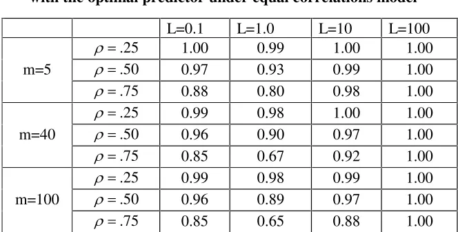
m MSE MSE with the limit decreasing to 0 as U increases to 1, showing that with many areas and large cross-sectional correlations, the loss in efficiency can be substantial. Table 1 shows the relative efficiencies ( *)/( ˆ)

i

i MSE

MSE

R T T for

Table 1: Relative efficiencies of working predictor compared with the optimal predictor under equal correlations model

L=0.1 L=1.0 L=10 L=100 25

.

U 1.00 0.99 1.00 1.00

m=5 U .50 0.97 0.93 0.99 1.00 75

.

U 0.88 0.80 0.98 1.00

25 .

U 0.99 0.98 1.00 1.00

m=40 U .50 0.96 0.90 0.97 1.00 75

.

U 0.85 0.67 0.92 1.00

25 .

U 0.99 0.98 0.99 1.00

m=100 U .50 0.96 0.89 0.97 1.00 75

.

U 0.85 0.65 0.88 1.00

For the second example we use the same working model but let _{( , )} |i k|

k i u

u

Corr 0

U to represent the true correlations among the random area effects. This correlation pattern corresponds to the case where the means y_i refer to different time points and the area effects follow the AR(1) model,

, ( ) 2 2 2/(1 2)

1 H H V V V U

U 2 1 Ÿ 1

u i

i i

i u Var

u . (7.5)

If i m signifies the last time point with observations, the optimal predictor of _Tm under this model is easily obtained by application of the recursive Kalman filter equations (Harvey 1989). For ‘large m’ the MSE of the optimal predictor can be computed explicitly by solving the corresponding Riccati equation. We find that

_(T*_{) {[(1U}2₎2_G4_4V2_V2_U2_(1U2_)]1/2_(1U2_)G2_}/2U2

u m

MSE . (7.6)

As in the previous example, the working predictor _Tˆ_i defined by (7.2) is unbiased under the

model (7.5) and as mof, _(Tˆ_)oJV2 i

MSE under both the working model and the true

model. Table 2 shows the relative efficiencies ( *)/( ˆ) i

i MSE

MSE

R T T for large m and different

values of _U and ( 2/ 2). u

L V V

Table 2: Relative efficiencies of working predictor compared with optimal predictor under Auto-regression model, large m

25 . 0

U 0.99 0.98 0.99 1.00

50 . 0

U 0.97 0.93 0.97 1.00

75 . 0

U 0.91 0.80 0.91 0.99

95 . 0

U 0.66 0.48 0.66 0.93

The first notable (but expected) result emerging from the two tables is that for fixed ratios L, R decreases as U increases, implying that the loss from using the working predictor increases. Yet, unless _U!0.5, Rt0.90. Another less expected result is that increasing L does

not necessarily imply a corresponding decrease in R. In fact, in both tables R decreases as L increases from 0.1 to 1 but then it increases when further increasing L. (It is easily shown that for the AR(1) model and for the limiting case mof under the equal correlations model,

) / 1 ( )

(L R L

R for all L, with the minimum value of R attained at L=1 for which J 0.5.) This result is explained by the fact that as _V2 _{increases in relation to} 2

u

V , more weight is assigned to the synthetic estimator y which is common to both the working and the true model so that the differences between the MSE of the two predictors diminish. The results presented in Table 2 for the AR(1) model are ‘one sided’ in the sense that the ‘borrowing of strength’ is only from previous occasions. We studied also the ‘two sided’ case where data collected before and after the time point of interest are used for deriving the optimal predictor and obtained very similar results.

The overall conclusion from this study is that unless the correlations between the area random effects are large, the loss in efficiency from using the working model is small. Notice

also that for small values of _U the MSE of the working predictor _Tˆ under the correct model _i

is similar to the MSE evaluated under the working model. Clearly, the results of this rather limited study need to be tested under different models.

8 Concluding remarks

where it is widely recognized that the use of model dependent inference is often inevitable. Given the growing