Volume 181 – No. 32, December 2018
Regional Decomposition of Images using Three
Parameter Logistic Type Mixture Model with K-Means
K. V. Satyanarayana
Department of Computer ScienceEngineering, Avanthi Institute of Engineering and Technology Narasipatnam, Visakhapatnam
K. Srinivasa Rao
Department of Statistics,Andhra University, Visakhapatnam
P. Srinivasa Rao
Department of Computer Scienceand Systems Engineering Andhra University, Visakhapatnam
ABSTRACT
For image analysis image decomposition or segmenting the images is a basic requirement. For decomposing the images probability models play a vital role. This paper addresses image decomposition using three parameter logistic type mixture distribution. Here it is assumed that the pixel intensities of image region follow a three parameter logistic type probability distribution. The estimation of parameters is carried utilizing Expectation and Maximization algorithm. The initialization of the parameters is done with K-means algorithm and moment method of estimation the number of image regions is obtained counting the peaks of the histogram drawn for the pixel intensities of the whole image. The decomposition algorithm (segmentation) is developed under maximum component likelihood function with Bayesian considerations. The efficiency of the proposed algorithm is studied by computing the metrics for segmentation such as GCE, VOI, PRI. The experimentation is conducted with five randomly chosen images taken from Berkeley image database revealed that the proposed algorithm is superior to the other model based segmentation algorithms for some images, which are having laptykurtic image regions.A comparative study with that of segmentation algorithm based on GMM is also presented.
Keywords
Image decomposition,Three parameter logistic type mixture distribution, Expectation and Maximization algorithm, Metrics of segmentation,K-means algorithm.
1.
INTRODUCTION
The image decomposition is the first step in image analysis which consider dividing the image into various image regions based on the features. The features of the grey images can be characterized by pixel intensities. There are several image segmentation(image decomposition) methods available for different types of images (K SrinivasaRao et al(2007),M seshashayee et al(2011),Chandra sekhar et al(2014)).In image decomposition usually it is considered that the pixel intensities of the images are modeled as Gaussian or Gaussian mixture model.(Yunjie Chen(2014),Celia A (2014),shanazAman et al(2015),Vamsikrishna M (2015), RajkumarG.V.S et al(2017)).All these authors assumed that the pixel intensities in each image region of the whole image are measokurtic,and hence Gaussian mixture model serve the purpose.
But in some images the distribution of the pixel intensities may not be measokurtic.Hence for effective image decomposition one has to consider alternative of Gaussian mixture model which accommodate laptykurtic and platy kurtic distributed image regions. RecentlySeshashayee et al(2014) and SrinivasaRao K et al(2014) have developed and
analyzed image segmentation algorithm based on new symmetric mixture distribution and generalized new symmetric mixture distributions.Jyothermayee et al ((2015),(2016),(2017)) have developed image segmentation methods using generalized laplace mixture models.The generalized laplacemixture model or the generalized new symmetric distribution includes various types of platykurticdistributions. However, in some images the pixel intensities may not be distributed aslaptykurtic. For this type of images the Gaussian mixture models or generalized new symmetric distribution or the generalized Laplace mixture models may not serve the purpose. Hence, in this paper we develop and analyze an image decomposition (segmentation) algorithm using three parameter logistic type mixture distribution. Here it is assumed that the pixel intensities of each image region follow three parameter logistic type distribution. The three parameter logistic type distribution includes several leptokurtic probability distributions. The rest of the paper is organized as follows: section-2 deals with three parameter logistic type distribution and its mixture model. The silent features of the mixture distribution are discussed. In section -3 the estimation of the parameters using Expectation and Maximization algorithm is discussed by deriving updated equations for the model parameters. In section-4the procedure for obtaining the initial values of the parameter through K-means algorithm and moment method of estimation is presented. In section-5 the image decomposition algorithm with component maximum likelihood under Bayesian considerations is developed. In section-6, the performance of the proposed algorithm is evaluated by computing the metrics of segmentation such as, PRI, VOC and GCE. In section-7 a comparative study of the proposed algorithm with that of GMM is given. Section-8 deals with conclusions and scope for further work in this direction of research.
2.
THREE PARAMETER LOGISTIC
TYPE DISTRIBUTION
2
2 2
2
3 (3 )
( , , ) (1)
1
, , 4
x
x x
p e
p f x
e
Where x p
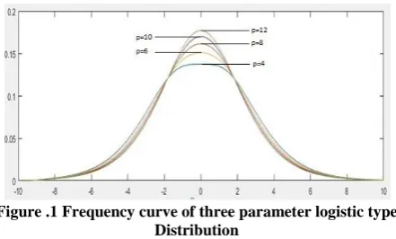
For various values of the parameters it generates the different shapes of probability curves associated with the three parameter logistic type distribution .The different shapes of frequency curves are shown inFigure1.
[image:2.595.57.278.214.347.2]Each value of the shape parameter
p
(4,5,6,7….) gives a bell shaped distribution.Figure .1 Frequency curve of three parameter logistic type Distribution
This distribution is symmetric about
and the distribution function is2
2
3 2
3
2 1 1
3 ( )
1
x x
x x
x x
e p e
p F X
e e
The entire image is the collection of regions, hence it is assumed that the pixel intensities of the entire image follows a k-component mixture of three parameter logistic type distribution and its probability density function is of the form.
2 1
( )
( , ,
)
(2)
k
i i
i
p x
f x
where k is the number of regions
0
i
1
are weights such that
i
1
andf x
i( , ,
2)
is given in equation (1).
iis the weight associated with ithregion in the whole image.The mean pixel intensity of the whole image is
1
(
)
Ki i i
E X
Even though the neighboring pixel intensities are correlated. The correlation can be made insignificant by considering spatial sampling proposed by Sewehand w. and Lei T (1992) and spatial averaging proposed by Kelley P.A. et al(1998).After reducing the correlations the pixel intensities are to be considered as independent .
3.
UPDATED EQUATIONS OF
EM-ALGORITHM FOR PARAMETER
ESTIMATION:
This section deals with the estimation of the model parameters. The Expectation and Maximization algorithm can be utilized for obtaining the estimates of the parameters involved in the model. The major consideration for EM algorithm is expectation of the likelihood function and then maximization of it with respect to the parameters. Following the heuristic arguments given by Jeff A. Bilmes(1997) the updated equations of the model parameters are obtained. This distribution of the pixel intensities of the image regions are having the three parameters namely
,
2,
p
the shape parameters is to be first established before utilizing the EM algorithm. Thep
can be estimated by equating the sample kurtosis with the population kurtosis. Let the sample kurtosis ism
3then
2 2
3 2
5 3
49
155
7 5
7
p
p
m
p
On simplification, we get
2
2
43 3 3
735 175 m p 2570 490 m p 775 343 m 0 (10) Solving equation (10) for
p
,we get
3
2 33 3
2570
490
4326400
967680
70 5
21 343
775
m
m
p
m
m
If
m
3
4.47089947 ,
Then we get two real roots and find out the value ofp
which is positive. After estimating the parameterp
the likelihood of the function of the sample observationsx x x
1,
2,
3...
x
N drawn from the image is( ) 1
( )
( ,
)
(3)
N
l s S
L
p x
( ) 1
1
( ) ( , (4)
N k
l
i i s
i s
L
f x
This implies
( )
1 1
log ( )
log
( ,
)
(5)
N k
l i i s
S i
L
f x
Where ,
i,
i2,
i
wherei
1, 2,3,...
n
2 2
2
1 1
3
(3
)
log ( )
log
(6)
1
s i i
s i i
x
s i
N m i
i
x
S i
i
x
p
e
p
L
e
Volume 181 – No. 32, December 2018
E-STEP
In the Expectation (E) step, the expectation value of log
( )
L
with respect to the initial parameter vector
(0) is( 0)
(0)
( ,
)
log ( ) /
(7)
Q
E
L
x
Given the initial parameters
(0). One can compute the probability density function of pixel intensity X as( ) ( )
1
( , ) ( , ) (8)
k
l l
s i i s
i
P x
f x
( )
1
( )
(
,
)
(9)
N
l s S
L
p x
( ) ( )
1 1
log ( ) log ( , ) (10)
N k
l l
i i s
S i
L f x
The conditional probability of any observations xs, belongs to
any region K is
( ) ( )
, ( )
( )
(
)
(
,
)
(11)
(
,
)
l l
k k s
l
k s l
i s
f
x
P x
p x
( ) ( )
, ( )
( ) ( )
1
(
)
(
,
)
(12)
(
,
)
l l
k k s
l
k s k
l l
i i s
i
f
x
p
x
f
x
The Expectation of the log likelihood function of the sample is
( )
( )
( ,
)
llog ( ) /
l
Q
E
L
x
But we have
( ) ( )
( ) ( )
2 ( )
2 ( )
( )
2 ( )
3
(3 )
( , ) (13)
1
l
s i
l i
l
s i
l i
x l
s i
l l
i s
x l
i
x
p e
p f x
e
This implies
( ) ( ) ( ) ( )
1 1
( ,
)
( ,
)(log
( ,
) log
)
(14)
k N
l l l l
i s i s i
i s
Q
P x
f x
M-STEP:
For obtaining the estimation of model parameters one has to maximize
Q
( ,
( )l)
such that
i
1
. This can be solved by applying the standard solution method for constrained maximum by constructing the first order Lagrange type function
( )
( )1
log (
)
1
(15)
k
l l
i i
F
E
L
where,
is Lagrangian multiplier combining the constraint with the log likelihood functions to be maximized. The above two steps are repeated as necessary, each iteration is guaranteed to increase the likelyhood and the algorithm is guaranteed to converge to a local maximum of the likelihood functionThe updated equations of
i for(
l
1)
thiteration is( 1) ( )
1
1
( ,
)
N
l l
i i s
s
P x
N
( ) ( ) , ( 1)
( ) ( ) 1
1
(
)
1
(16)
( ,
)
l l
N
l l s
l
l k
l l
s
i i s
i
f x
N
f x
For updating the parameter
i,
i
1, 2,3...
k
we consider the derivatives ofQ
( ,
( )l)
with respect to
i and equal to zeroWe have
Q
( ,
( )l)
E
log ( ,
L
( )l)
There fore ( )
( ( ,
l))
0
i
Q
Implies
( )
(log ( ,
l))
0
i
E
L
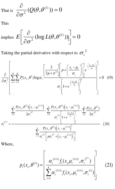
Taking the partial derivative with respect to
i,we have2
2
. 2
1 1
3 3
( , ) log 0 (17)
1
s i i
s i i
x
s i
N K i
l
i s i
x
s i
i
i
x
p e
p P x
e
( ) ( )
. . .
( ) 2
( )
1 2 ( ) 1 1
( ) ( )
(1)
. 2 ( )
1 2 ( )
( )
( , ) 2 ( , ) 2 ( , )
( ) 1
(18)
( , )
2
( )
l s i l i
l l l
n n n
i s s i s i s
l x
l
s l s i s i s l
i l i
i l
i n l
i s l s l
s i i l
i
P x x P x P x
x
p e
P x
x p
That is ( )
2
( ( ,
))
0
l
Q
Thisimplies ( )
2
(log ( ,
))
0
l
E
L
Taking the partial derivative with respect to
i22
2
. 2
2
1 1
3 3
( , ) log 0 (19)
1
s i i
s i i
x
s i
N K i
l
i s i
x s i
i
i
x
p e
p P x
e
1
1 1
. . .
3 2
1 1 1
3
2
2 1 .
2 1
4 2
1
( , ) ( , ) ( , )
2 2
1
20 ( , )
l l
s i l
i l
l l
l l l l l
N N N
i s s i i s s i i s
x
s i s s i
i
i
l l
N
i s s i
l s
i i s i
P x x P x x P x
e P x x
p x
Where,
( )
( 1) ( 1) 2
, ( )
( 1) ( 1) ( )
1
(
,
)
( ,
)
(21)
( ,
,
)
l
l l
i i s i i
l
i s k
l l l
i i s i i
i
f x
p x
f x
4.
INITIALIZATION OF THE
PARAMETERS BY K-MEANS:
The efficiency of the EM algorithm in estimating the parameters is heavily dependent on the number of regions in the image .The number of image regions are obtained, by plotting the histogram of the pixel intensities of the whole image, and the number of peaks in the histogram are taken as the number of regions say ‘k’
A commonly used method in initializing parameters is by drawing a random sample from the entire image (McLachan G. AND Peel D.(2000). This method performs well, if the sample size is small. To overcome this problem we use the K-means algorithm to divide the whole image into homogeneous regions.
We obtain the initial estimates of
i,
i2 and
i for the ith region with the moment method for three parameter logistic distributionThe initial estimates of the parameters are
i=1
k
, where i=1,2,3…k.
i
X
, and 24
3(
1)
i i
i
n
n
S2, where S2 is sample variance, ni is the number of observations in the ith
segmentation.
5.
IMAGE DECOMPOSITION
ALGORITHEM:
The image segmentation algorithm is proposed in this section. The model parameters are estimated as discussed in section 2 and 3. To segment we allocate the pixels to the respective image regions. The major steps in image segmentation are as follows:
Step 1:- K-means algorithm is utilized for dividing pixel intensities of the whole image into k-image regions. Where k is number of image regions.
Step 2:-compute the initial estimates for the parameters of the model using moment method of estimation for each image region as discussed in section-3.
Step3:- The Expectation and Maximization algorithm with the updated equations of parameters given in section-2 is utilized for computing the final parameters of model.
Step-4:-The allocation of each pixel in the whole image into its corresponding jth image region is done by computing the
component maximum likelihood of the each image region as follows:
i.e.,
x
sis assigned to the jth region for which Lj is maximum.Where
2
2
2
2
3
(3
)
,
1
,
,
4
s i
i
s i
i
x
s i
i j
x
i
i i
x
p
e
p
L
MAX
e
p
6.
EXPERIMENTATION
AND
RESULTS
This section deals with the experimentation of the suggested image decomposition algorithm. The experiment is carried with five randomly taken images namely, OSTRICH,WOMAN, HILL,OCEAN and EAGLE from
Berkeley image data
[image:4.595.52.288.68.455.2]base(http://www.eees.berkeley.edu/Research/Projects/CS/Visi on/bsds/BSDS300/html).The feature of the images are obtained by considering pixel intensities. The pixel intensities are obtaining by using MATLAB. Assuming that pixel intensities of image regions follow a mixture of three parameter logistic type distribution, the model characterizing the whole image is developed. With the help of K-means algorithm, the number of image regions ‘k’ for each image is obtained and presented in Table.1
Table 1.1: Refined values of K (K-means Algorithm)
IMAGE OSTRIC H
WOMA N
OCEA N
HILL S
EAGL E Estimat
e of K 2 3 3 4 2
With the pixel intensities of each image region the starting values for the model parameters
i,
i2 and
i whereVolume 181 – No. 32, December 2018
1.3, 1.4, 1.5 and 1.6 for different images. With these initial values of the parameters and the Expectation and Maximization algorithm, the refined estimates of parameters are obtained and shown in Tables:2,3,4,5 and 6
Table:1.2 ML Estimates for Ostrich data for(K=2)
Parameters Initial Parameters Refined estimates Image Region Image Region
1 2 1 2
αi 0.500 0.500 0.2591 0.7409
µi 40.5146 113.260 81.456 248.14
σi2 64.09627 141.798 458.4785 1214.7420
For each image region the parameter
p
is first estimated asp
ˆ
4
Histogram, k=2 Gray Image Segmented Image
Table:1.3 Estimates of the parameters for WOMAN Image
Parame ters
Initial Parameters Refined estimates Image Region Image Region
1 2 3 1 2 3
α 0.333 0.333 0.333 0.120 5
0.617 7
0.261 8 219.6
327
115.5 619
71.72 64
54.25 48.14 160.2 3
σ 920.5
615
406.2 072
5738. 391
355.4 58
498.2 58
1958. 21
Histogram, k=3 Gray Image Segmented Image
Table:1.4 Estimate of the parameters for OCEAN Image
Pa ra M e ter s
Initial Parameters Refined estimates Image Region Image Region
1 2 3 1 2 3
α 0.333 0.333 0.333 0.2402 0.57 0.18
11 87 73.197
8
125.46 05
189.78 68
72.99 461. 91
781. 25 σ 287.40
86
166.94 6
135.25 7
240.21 54
571. 45
188. 27
Histogram, k=3 Gray Image Segmented Image
Table:1.5 Estimates of the parameters for HILLS Image
P ar a M e te rs
Initial values of the Parameters
Refined Estimates
Image Region Image Region
1 2 3 4 1 2 3 4
αi 0.25 0.2
5
0.25 0.25 0.18 15
0.41 76
0.20 29
0.19 80 µi 189.
422 3
58. 928 2
107. 530
0 154. 664
0 249.
251 649.
472 440.
615 372. 725
σi 2
238. 851 1
364 .34
152. 816
7 130. 238
3 298.
457 4
425. 879 5
114. 528 7
181. 254
1
Histogram, k=4 Gray Image Segmented Image
Table::1.6 TPLTM ML Estimates for EAGLE data for (K=2)
Parameters Initial Parameters Refined estimates Image Region Image Region
1 2 1 2
αi 0.500 0.500 0.0635 0.9365 i 40.5146 113.2603 23.11 99.33
Histogram, k=2 Gray Image Segmented Image
The fitted P.D.F of OSTRICH is
81.456 2 21.412112 2 2 81.456 21.412112 2 2 81.456 3 21.412112 (3 )
( , ) (0.2591)
21.412112 1 248.14 3 34.853191 (3 ) (0.7409) s s x s l s x s x p e p f x e x p p 248.14 34.853191 2 248.14 34.853191 34.853191 1 s s x x e e
The fitted P.D.F of EAGLE is
23.11 2 7.953239 2 2 23.11 7.953239 2 2 23.11 3 7.953239 (3 )( , ) (0.0635)
7.953239 1 99.33 3 13.463172 (3 ) (0.9365) s s x s l s x s x p e p f x e x p e p
99.33 13.463172 2 99.33 13.463172 13.463172 1 s s x x e The fitted P.D.F of OCEAN is
54.25 2 18.853594 2 2 54.25 18.853594 2 2 54.25 3 18.853594 (3 )( , ) (0.1205)
18.853594 1 48.14 3 22.321694 (3 ) (0.6177) s s x s l s x s x p e p f x e x p p
48.14 22.321694 2 48.14 22.321694 160.23 2 44.251667 2 160.23 44.251667 22.321694 1 160.23 3 44.251667 (3 ) (0.2618) 44.251667 1 s s s s x x x s x e e x p e p e 2 The fitted P.D.F of WOMAN is
72.99 2 15.49884 2 2 72.99 15.49884 2 2 72.99 3 15.49884 (3 )
( , ) (0.2402)
15.49884 1 461.91 3 23.905021 (3 ) (0.5711) s s x s l s x s x p e p f x e x p e p 461.91 23.905021 2 461.91 23.905021 781.25 2 13.721156 2 781.25 13.721156 23.905021 1 781.25 3 13.721156 (3 ) (0.1887) 13.721156 1 s s s s x x x s x e x p e p e 2
The fitted P.D.F of HILLS is
249.251 2 17.275920 2 2 249.251 17.275920 2 249.251 3 17.275920 (3 )
( , ) (0.1815)
17.275920 1 649.472 3 20.636849 (3 ) (0.4176) s s x s l s x s x p e p f x e x p p 649.472 2 20.636849 2 649.472 20.636849 440.615 2 10.701809 2 440. 20.636849 1 440.615 3 10.701809 (3 ) (0.2029) 10.701809 1 s s s s x x x s x e e x p e p e 2 615 10.701809 372.725 2 13.463065 2 2 372.725 13.463065 372.725 3 13.463065 (3 ) (0.1980) 13.463065 1 s s x s x x p e p e
7.
COMPARITIVE STUDY OF THE
ALGORITHM:-This section deals with the performance of the proposed algorithm for image decomposition. The image segmentation quality metrics such as probabilistic rand index (PRI), global consistency error (GCE), and variation of information (VOI) are utilized. Table 7 provides the comparative image segmentation metrics obtained for the five images under experimentation with respective for the proposed algorithm and that of algorithm with GMM
Table:7 SEGMENTATION PERFORMANCE MEASURES
IMAGE
S METHOD
PERFORMANCE MEASURES
PRI GCE VOI
OSTRI CH
GMM 0.914
7
0.2785 0.4273
3 parameter -K Means
0.925 1
Volume 181 – No. 32, December 2018
WOMA N
GMM 0.887
6
0.0232 0.1417
3 parameter -K Means
0.910 4
0.0199 0.1441
OCEAN
GMM 0.885
2 0.0339 0.1927 3 parameter -K
Means
0.914
5 0.0142 0.1214
HILLS
GMM 0.868
8 0.2572 0.3357 3 parameter -K
Means
0.915 4
0.1541 0.2347
EAGLE
GMM 0.998
7 0.0023 0.0126 3 parameter -K
Means
0.999
1 0.0014 0.0049
The Table.7 reveals that the proposed segmentation algorithm is much superior to that of segmentation algorithm with GMM with respect to the image segmentation quality metrics PRI,GCE, and VOI. For the images OSTRICH,WOMAN, HILL,OCEAN and EAGLE. Further the efficiency of the proposed segmentation algorithm is also studied by obtaining image quality metrics such as Average Difference, Maximum Distance, Image Fidelity, Mean Square Error, Signal to Noise Ratio, Image Quality Index. Table 6.2 presents the image quality metrics for the five images with respect to the proposed algorithm and the segmentation algorithm with GMM.
Table.8 presents the quality metrics of image segmentation with three parameter logistic type mixture model and K-means algorithm
Table.8 Quality Metrics for Comparison
IMAGES Quality Metrics GMM Proposed
3parameter-K-means
OSTRICH
Average Difference
0.5315 0.4865
Maximum Distance
0.4763 0.5715
Image Fidelity 0.8124 0.8978 Mean Square
Error
0.0770 0.0592
Signal to Noise Ratio
14.080 24.215
Image Quality Index
0.8460 0.9021
WOMAN
Average Difference
0.4860 0.5845
Maximum Distance
0.9435 0.9814
Image Fidelity 0.4620 0.4928 Mean Square 0.0803 0.0548
Error
Signal to Noise Ratio
4.7261 5.1878
Image Quality Index
0.9782 0.9914
OCEAN
Average Difference
0.3211 0.1854
Maximum Distance
0.6810 0.7514
Image Fidelity 0.6885 0.8214 Mean Square
Error
0.0645 0.0324
Signal to Noise Ratio
4.0802 5.879
Image Quality Index
0.7763 0.8947
HILLS
Average Difference
0.2664 0.0958
Maximum Distance
0.7664 0.8914
Image Fidelity 0.9348 0.9856 Mean Square
Error
0.0138 0.0111
Signal to Noise Ratio
0.9383 2.1987
Image Quality Index
0.5710 0.6347
EAGLE
Average Difference
0.2350 0.3502
Maximum Distance
0.5925 0.7817
Image Fidelity 0.9882 0.9978 Mean Square
Error
0.0038 0.0011
Signal to Noise Ratio
11.1494 19.245
Image Quality Index
0.9869 0.9916
The Table.8 provides evidences for superiority of image segmentation algorithm with mixture of three component logistic probability distribution and K-means algorithm than the other algorithms under study. The quality metrics of proposed algorithm for the experimental images are very close to the standard values of the metrics.
8.
CONCLUSIONS
developed with component maximum likelihood by considering Bayesian frame work. The experimentation conducted with five images randomly taken from Berkeley image database revealed that the proposed image decomposition method outperforms, the existing image segmentation method for the grey images having leptokurtic pixel intensities in image regions. It is also observed that through segmentation quality metrics the proposed algorithm is superior than the segmentation algorithm based on GMM. The proposed algorithm is useful in decomposing the images at medical diagnostics, security and surveillances, remote sensing. The image decomposition using this algorithm further extended to color images by considering multivariate feature vector with multivariate three parameter logistic type mixture model, which will be taken up elsewhere.
9.
REFERENCES
[1] Srinivas.Y and SrinivasRao.K (2007), “Unsupervised image segmentation using finite doubly truncated Gaussian mixture model and Hierarchical clustering ”, Journal of Current Science,Vol.93,No.4, pp.507-514. [2] T. Yamazaki (1998) “Introduction of algorithm into
color image segmentation,” Proceedings of ICIRS’98, pp. 368–371
[3] T.Lie et al.(1993), “ Performance evaluation of Finite normal mixture model based image segmentation, IEEE Transactions on Image processing, Vol.12(10), pp 1153-1169.
[4] Z.H.Zhang et al (2003).“ EM Algorithms for Gaussian Mixtures with Split-and-mergeOperation”, Pattern Recognition, Vol. 36(9),pp1973-1983.
[5] T. Jyothirmayi, et al(2016)., “Image Segmentation Based on Doubly Truncated Generalized Laplace Mixture Model and K Means Clustering International Journal of Electrical and Computer Engineering (IJECE), Vol. 6, No. 5, October 2016, pp. 2188~2196.
[6] T. Jyothirmayi, et al (2017).,“Performance Evaluation of Image Segmentation Method based on Doubly Truncated Generalized Laplace Mixture Model and Hierarchical Clustering” .J. Image, Graphics and Signal Processing, 2017, 1, 41-49
[7] The Berkeley segmentation dataset http://www.eecs.berkeley.edu/Research/Projects/ CS/vision/bsds/BSDS300/html/dataset/images.html.
[8] SrinivasRao. K,C.V.S.R.Vijay Kumar, J.LakshmiNarayana, (1997) “ On a New Symmetrical Distribution ”, Journal of Indian Society for Agricultural Statistics, Vol.50(1), pp 95-102
[9] M.Seshashayee, K.Srinivasarao, Ch.Satyanarayana and P.Srinivasarao- (2011) – Studies on Image Segmentation method Based on a New Symmetric Mixture Model with K – Means, Global journal of Computer Science and Technology, Vol.11, No.18, pp.51-58. ISSN: 0975-4172,0975-4350
[10]GVS.Rajkumar, K.Srinivasarao, and P.Srinivasarao-(2011) – Studies on color Image segmentation technique based on finite left truncated Bivariate Gaussian mixture model with k - means, Global Journal of computer Science and Technology, Vol.11, No.18, pp 21- 30. ISSN: 0975-4172,0975-4350
[11] GVS.Rajkumar K.Srinivasa Rao P.Srinivasarao (2011)studies on color image segmentation technique based on finite left truncated bivariate Gaussian mixture model with k-means, global journal of computer science and technology, vol.11, no.18. Issn: 4172, 0975-4350
[12] Mclanchlan G. And Krishnan T (1997)., “ The EM Algorithm and Extensions”, John Wiley and Sons, New York -1997.
[13] Mclanchlan G. and Peel.D (2000), “ The EM Algorithm For Parameter Estimations”, John Wiley and Sons, New York -2000.
[14] Jeff A.Bilmes (1997), “ A Gentle Tutorial of the EM Algorithm and its application to Parameter Estimation for Gaussian Mixture and Hidden Markov Models”, Technical Report, University of Berkeley, ICSI-TR-97-021.
[15]R.Unnikrishnan, C,Pantofaru, and M.Hernbert ( 2007), “ Toward objective evaluation of image segmentation algorithms,” IEEE Trans. Pattern Analysis and Machine Intelligence . Vol.29, no.6, pp.929-944.
10.
AUTHOR’S PROFILE
Prof K.Srinivasa Rao did his M.sc and PhD in statistics from
Andhra University Visakhapatnam. He is having 33 years of teaching and research experience. He published 193 research papers in reputed journals he was the former chief editor of JISPS and associate editor OPSEARCH., He was former chairman PG board of studies, head of the department and Dean Research & Development of Andhra University presently he is the member secretary APSET. He guided 47 students for PhD degrees in statistics, computer science and mathematics. His current areas of research are communication networks, stochastic modeling and data analysis.
Dr. Peri. Srinivasa Rao is presentlyworking as Professor in
the Department of Computer Science and Systems Engineering, Andhra University, Visakhapatnam. He got his Ph.D degree from Indian Institute of Technology, Kharagpur in Computer Science in 1987.
He published several research papers and delivered invited lectures at various conferences, seminars and workshops. He guided a number of students for their Ph.D and M.Tech degrees in Computer Science and Engineering and Information Technology. His current research interests are Image Processing, Communication networks, Data Mining and Computer Morphology.
K.V.Styanarayanais presently working as Assistant
Professor in the department of Computer Science and Engineering,Avanthi Inistitute Of Engineeringand Techonology, Narasiparnam Visakhapatnam. He presented research papers in national and