Rapid Algorithm for Independent Component Analysis

Rapid Algorithm for Independent Component Analysis

Ryota Yokote, Yasuo Matsuyama

Department of Computer Science and Engineering, Waseda University, Tokyo, Japan. Email: rrryokote@wiz.cs.waseda.ac.jp, yasuo2@waseda.jp

Received March 30th_{, 2012; revised May 2}nd_{, 2012; accepted May 10}th_{, 2012}

ABSTRACT

A class of rapid algorithms for independent component analysis (ICA) is presented. This method utilizes multi-step past information with respect to an existing fixed-point style for increasing the non-Gaussianity. This can be viewed as the addition of a variable-size momentum term. The use of past information comes from the idea of surrogate optimization. There is little additional cost for either software design or runtime execution when past information is included. The speed of the algorithm is evaluated on both simulated and real-world data. The real-world data includes color images and electroencephalograms (EEGs), which are an important source of data on human-computer interactions. From these experiments, it is found that the method we present here, the RapidICA, performs quickly, especially for the demixing of super-Gaussian signals.

Keywords: Independent Component Analysis; Speedup; Past Information; Momentum; Super-Gaussian; Negentropy

1. Introduction

Optimization of the amount of information leads to a rich class of learning algorithms for various types of signal processing. The learning phase is usually iterative, which is often the cause of their effective-but-slow nature. The speed of a learning algorithm is important, because this facilitates the application to real-world problems. Inde-pendent component analysis (ICA) [1] is a typical exam-ple of such an algorithm. Among the various ICA meth-ods, the FastICA, which is a fixed-point algorithm [2], is the most popular one because it usually out-performs the fastest version of the gradient-style algorithms [3-5]. However, the need for ever faster ICAs has arisen ubiq-uitously [6,7].

Reflecting this necessity for speedup, this paper pre- sents a class of rapid ICA algorithms. The core idea is the introduction of past information to the fixed-point ICA. This method inherits the idea for the speedup of the gradient-style algorithm using a surrogate function [3-5].

When a new class of learning algorithms is presented, it is necessary to check the following:

1) Is its merit on the performance enough?

2) Is it applicable to substantial real-world problems? In this paper, we present the RapidICA algorithm and the results of testing it on both artificial and real-world data. As practical data, we adopted color images and electroencephalograms (EEGs) for pattern recognition. After extensive experiments, the effectiveness of the RapidICA over the existing fixed-point ICA can be fully

recognized.

The organization of this paper is as follows. In Section 2, preliminaries to the ICA problem are given. Section 3 shows three types of fast versions, starting with the sim- plest one. Next, a summarized version is given, along with a strategy for stabilization and a measure of the convergence. Section 4 presents the results of experi- ments comparing the RapidICA with the FastICA for both artificial and real-world data. The practical data were color images and electroencephalograms (EEGs). In Section 5, concluding remarks are given.

2. Preliminaries to ICA

2.1. Formulation of ICA

In this section, we present our notation and the minimum necessary preliminaries for ICA. Given a measured ran- dom vector x, the problem of ICA starts with the rela-

tionship of the superposition.



x As (1)

Here,



1, ,

T n



x x



x  (2)

is zero mean. The matrix A is an n × n unknown non-

singular matrix. The column vector



1, ,

T n



s s



s  (3)

dependent of each other, and to be non-Gaussian except for one component. The necessity of these assumptions indicates the following:

1) For the consistency of the ICA problem, it is desir- able that the xi are far from a Gaussian distribution.

2) There are two classes that are non-Gaussian. One is super-Gaussian and the other is sub-Gaussian. But by the central limit theorem, the summation of only a few inde- pendent sub-Gaussian random variables easily becomes an almost Gaussian one. Therefore, real-world sub-Gauss- ian mixtures xi for ICA applications are rare. On the other

hand, super-Gaussian mixtures xi are found in many

sig-nal processing sources. Thus, experiments on real-world data will be mainly on super-Gaussian mixtures.

Using the data production mechanism of (1)-(3), the problem of ICA is to estimate both A and s using only x.

This is, however, a semi-parametric problem where un- certainty remains. Therefore, we will be satisfied if the following y and W are successfully obtained.



1, ,





1, ,



T T

n n

y y w w

  

y  Wx  x (4)

Here, the random vector y is an estimated column

vector with independent components. Note that the or- dering of components of y is allowed to be permuted

from that of s. The amplitude of si is also uncertain in this

generic ICA formulation. Therefore, W is an estimation

of 1

A



 . Here, is a nonsingular diagonal matrix,

and is a permutation matrix.



2.2. Cost Functions for Independence

There are several cost functions that measure the inde-pendence of random variables. A popular target function is the minimization of the Kullback-Leibler divergence, or, equivalently, the minimum average mutual informa-tion. The methods we present in this paper are related to this information measure.

2.2.1. Minimum Average Mutual Information and Its Extension

As is well known from information theory [8], the aver- age mutual information works as a directed distance be- tween two probability densities of a Kullback-Leibler divergence. By choosing a probability density function (pdf) q to be an independent one, the cost function to be minimized is expressed as follows.





 

 

_

 

_

1 1 1 1

log d 0

, ,

n i i

n

n i i i

i i i Y

n

I Y D q p

q y q y

p y y

             







y   (5)

This average mutual information becomes zero if and only if the i are independent of each other. Thus dif-

ferentiation with respect to W leads to a gradient descent

algorithm. This method can be generalized by using a convex divergence that includes the average mutual in- formation of (5) as a special case.

y

The convex divergence is an information quantity ex- pressed as follows [9].

 





_

 

_

 





 

 

1 1 1 1 1 1

, , d

, , , , d 0 n i i i

f _Y n

n

n n

i i n

i Y i i i g q y D p q p y y f

p y y

p y y q y g

q y

D q p

                      









_

y y    (6)

Here, f r

 

is convex on r



0,



, and

 

 

1

g r rf r is a dual convex function. Note that the special case of

 

log1

f r r

 (7)

is reduced to the average mutual information (5). The differentiation of D q p_g

 

with respect to W leads to a

gradient descent update for the demixing matrix [5].



t 1



 

t  g

W W  W

 

t (8)

 

 





 





 



 



 





















g g c g

T

T c

t t t

t t t t

t t t

                 _       _{ }

W W W

I y y W

I y y W

  

(9)

Here, t is the iteration index for the update, and  is a delay. The symbol g represents a natural gradient of

g in Equation (6) multiplied by , where c is a

positive constant associated with the Fisher information matrix [10].

T cW W

 

t

 0 is a design parameter. I is the

identity matrix. The matrix

 

 

 

 

 

 

 

1 1 1 1 1 1 , , , , T n n n n n n y y q y q y

q y q y

 _{ }  _           y 

 (10)

is unknown in practice since is unknown in the

formulation of the ICA. Therefore, in practical ICA exe- cution, the function

 

i i

q y

 

i yi

 is assumed to be a nonlinear

one, such as 

 

y _y3

i i  i or i

 

yi tanhyi.

which is based on the non-Gaussianity maximization.

2.2.2. Non-Gaussianity Maximization Based upon Approximated Negentropy

Non-Gaussianity can be measured by the Kullback-

Leibler divergence (5) from a pdf to a

Gaussian pdf , which is called

negen-tropy.



1, , n



p y  y



Gauss 1, , n

p y  y



 















 

1 Gauss 1

Gauss

, , _n , , _n



J D p y y p y y

H H



 

y

y y

 

(11)

A criterion for the ICA of Equation (4) can be set to the maximization of the negentropy (11). It is not possible

to maximize the negentropy directly since 1



is unknown. Therefore, in the FastICA [2], the negen- tropy maximization is approximated. For this approxima- tion, we pose an assumption that the xi are pre-whitened

to be uncorrelated with each other.



, , n

p y  y

T

E_xx  _ I (12)

Note that this assumption was not needed in the method of Section 2.2.1.

Then, using a predetermined contrast function G y

 

, the maximization of (11) is approximated by the follow- ing optimization with constraint [2].

 

 





  

2 1

Maximize

wrt , 1, ,

under

n T

i i

i

T T

j k jk

E G E G

i n

E





       

 _{ }

 



w x

w

w x w x

 (13)

Here,  is a zero-mean, unit-variance Gaussian ran- dom variable. By virtue of the above drastic approxima- tion, the FastICA with a couple of variants [2] is ob- tained.





2





*

,

and then / for all

i i iT i Ti i i

i i i

E G E G

i



 

  

 _  _ _



w x w x w x w

w w w



 ₍₁₄₎

Here, and are the first and second deriva-

tives of a contract function

G

 _2_G

 

G y . Examples of G y

 

are y4_{, log cosh y, and exp}



_y2 ₂



_{. The update method}

(14) is a fixed-point algorithm and, because of its speed, it is the current de facto standard for ICA.

2.2.3. Mediation between Gradient Descent and Fixed-Point Algorithms for Speedup

So far, two preliminary sections have been presented. The first one, Section 2.2.2, presents a direct minimiza- tion of the convex divergence between the current and independent pdfs. The last term of the last line of Equa- tion (9) is the important one.

1) This term, which depends on the past information,

is the core of the speedup [10].

2) The case of c0 corresponds to the optimiza-

tion of the Kullback-Leibler divergence or its subsidiary, the entropy.

The second preliminary, the FastICA derived from the entropy difference, updates Equation (14) in a fixed- point style. Based upon the theoretical foundation of the derivation of Equation (9), one may conjecture that the acceleration methods for Equation (14) would be obtain- able by using the strategy of Equation (9). The rest of this paper will show that this conjecture is answered in the affirmative. We comment here in advance that the process we use to obtain the accelerated version of the fixed-point method is not naïve. It requires more artifice than the method of Section 2.2.1 since orthonormaliza- tion steps need to be interleaved. But we will see that the result will be easy to code as software.

3. Rapid Methods for ICA

In this section, several steps towards the final rapid ver-sion are presented. From this point on, the description will be more software oriented.

3.1. Observed Signal Preprocessing and Additive Update Expression

Instead of the measured vector x, its whitened version z,

obtained in the following way, is used as a target source to be demixed.



z Vx (15)



1 2 1 2

1, ,

T T

m

 

 

V D E D e  e



(16)

Here, D is the diagonal matrix constructed from the

largest m n eigenvalues of the covariance matrix

T

E_xx _, and ei, i1, , m, are the corresponding ei-

gen-vectors. Then, the update and orthonormalization steps of the fixed-point method are expressed as follows:

Update step: W is updated by the following computa-

tion.

 

T _diag



2

 



i

E G  E G y 

 _ _ _ _

W y z W (17)

Orthonormalization step: W is orthonormalized by us-

ing the eigenvalue decomposition.



_T



1 2



W WW W (18)

Since we will use the speedup method of Section 2.2.1, it is necessary to rewrite (17) as an additive form.

 



2



 

diag 1 T

i

E G y  E G 

  _ _{ } _

W W y z (19)

Equation (19) can be derived by dividing the right-

hand side of Equation (14) by . This is

allowed since the orthonormalization step for

 

W follows.

2 T

i

E G 

Then the basic method, which is the FastICA, is de- scribed as follows:

[Basic Method] Step 1: yWz

Step 2: _{diag 1}



2

 



 

T

i

E G y  E G

  _ _{ } 

W W y z _

Step 3: _



T



1 2

W WW W

Beginning in the next subsection, a series of speedup versions is presented. Findings in each version are sup- ported by extensive experiments. Except for the destina-tion algorithm, intermediate experimental results are omitted in order to save space.

3.2. High-Speed Version I

For the basic method, which is the FastICA, it has been pointed out that the orthonormalization of Step 3 some- times hinders the learning of non-Gaussianity by causing a slow convergence. Therefore, we start by considering an algorithm that simply increases the update amount.

[Method 0: Naïve version] Step 1: yWz

Step 2: _{diag 1}



2

 



 

T

i

E G y  E G 

W   _ _{ } y z _

Step 3: W W 



1 



W

Step 4: _{W }



_WWT



1 2_W

This naïve method is too simple, in that convergence will frequently fail for unadjusted 0, even for small figures. Therefore, we make this increase usable by in- serting an orthonormalization step.

[Method 1: Opening version] Step 1: yWz

Step 2: _{diag 1}



2

 



 

T

i

E G y  E G 

W   _ _{ } y z _

Step 3: W W W

Step 4: _



T



1 2

W WW W

Step 5: W W  W

Step 6: _



T



1 2

W WW W

One might think that this version simply computes the same update twice, but the following observations lead us to better versions:

1) Step 2 requires much more computational power than do the others.

2) Without Step 4, the increase by 0 could cause oscillations.

3.3. High-Speed Version II

By integrating Method 1 and the usage of the past infor- mation described in Section 2.2.1, the following method is derived.

[Method 2: Second-order version] Step 1: yWz

Step 2: WoldW

Step 3: _{diag 1}



2

 



 

T

i

E G y  E G

  _ _{ }

W W y z 

Step 4: _{W }



_WWT



1 2_W

Step 5: W WWold

Step 6: W W   W

Step 7: _



T



1 2

W WW W

The key point of this method is that there are two types of increments. The first type is in Step 3 and the second one is in Step 6. This method has the following proper-ties:

1) Each increment uses different time information. This is equivalent to the usage of a higher-order strategy.

2) The computed increments of Step 5 gradu-

ally converge to the null matrix O. Therefore, this

method is more stable than Method 1.

W

3) The computational load of Step 5 is negligible compared to that of Step 3. Therefore, the reduction of iterations will be directly reflected in the runtime speed- up.

3.4. High-Speed Version III

In High-speed Version II, the adjusting parameter 0

of the increment was a scalar, such as 0.1. The next step is to find reasonable values of i0 that depend on the

row indices i of W.

[Method 3: Variable step-size version] Step 1: yWz

Step 2: WoldW

Step 3: _{diag 1}



2

 



 

T

i

E G y  E G

  _ _{ }

W W y z 

Step 4: _



T



1 2

W WW W

Step 5: W WWold

Step 6: W W diag

 

i W

Step 7: _



T



1 2

W WW W

rent and past information.

,old ,old

max i , i ,0

i

i i

     

   

 

w w

w w (20)

Equation (20) has the property that a large change in the direction of wi from wi,old causes the value of

0

i

  to be small. This property is useful in helping to avoid oscillations during the intermediate steps. However, the magnitude of i is not taken into account. Also,

near to the convergence maximum, the value of

w

0

i  

might become numerically unstable since division by zero could occur. We now get to the final form.







2 ,old2



2 ,old

max , ,0

max ,

i i i

i i

 

  



  

w w

w w

(21)

Here,  0 is a constant, but it can be omitted (i.e.,

1

  ). The constant  0 serves the purpose of pro-viding numerical stability by preventing division by zero

( for 32-bit machines). Equation (21) has the

following properties:

2

 ₁₀6

1) When i and i,old are close together, the

value of i w

0

w

  is large since this direction needs to be emphasized. On the other hand, if the directions of wi

and i,old are considerably different (the extreme case

is anti-parallel), the value of

w

0

i

  is close to zero.

2) Because of _2_{, a small generates a small}

i w

0

i   .

Properties 1) and 2) give us hope that considerable speedup can be obtained with very little increase in computational complexity. There is one more property on which to comment.

3) It should be noted that every ICA algorithm has the possibility of non-convergence. The FastICA [2] is not an exception [6]. There are many sources that cause this, and one can easily generate such a case by using data that is non-Gaussian but almost Gaussian. In such a case, a little bit of a slowdown greatly helps the stability.

 



2



 

diag 1 T

i

E G y E G

   

  _ _{ }

W W y z 



(22)

Here,  



0,1 is a slowdown constant. The case of 1.0

 

0.98

is the FastICA, which may not converge on some data. In our preliminary experiments with Method

3,   1.0 worked well in achieving convergence

without too much slowdown.

3.5. Total Algorithm: The RapidICA

Up to this point, we have presented steps that increase the speedup and stabilization. Integrating all these steps is expected to produce an even faster ICA than the exist- ing ones. The following procedure summarizes the Rapid- ICA.

[RapidICA] Step 1: yWz

Step 2: WoldW

Step 3: W W  W1

where

 



2



 

1 diag 1

T i

E G y E G

    

W   _ _{ } y z _

Step 4: _



T



1 2

W WW W

Step 5: W2,old W2

Step 6: W2W Wold

Step 7: W W diag

 

i W2

with i of Equation (21).

Step 8: _



T



1 2

W WW W

In the appendix, we will give the source code of the RapidICA in the programming language R.

It is important to emphasize the following:

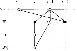
1) The algorithm of the RapidICA utilizes past infor- mation over three steps in a single cycle. This is illus- trated in Figure 1. Let the iteration index be denoted by t.

Given the demixing matrix , an estimation of the

independent component is computed. This step

requires the most computation. This

 

t W

 

t y

 

t

y is then used to

compute W1

 

t . By orthonormalization, W

 

t

pro-ceeds to W



t1



. Then, this W



t1



together with

 

t

W is used in the computation of W2

 

t . Finally,



t2



W is computed by using W



t1



, W2



t1



,

and W2



t1



, which was saved as old. Thus, the

RapidICA uses the update information from up to three prior steps. Note that the RapidICA of Method 2 (con-stant step coefficient) lacks the arrow from

W



1



2 t

W 

to W



t2



. Therefore, the RapidICA of Method 2 makes use of past information of no more than two prior steps.

2) From Figure 1, one may be reminded of the use of

a momentum variable with a dynamical system to turn it into a learning system [11]. The use of a momentum term appears in various iterative methods. The FastICA is not

1

t t t1 t2

2

W

W

y

1

[image:5.595.344.507.610.718.2]

W

an exception, since acceleration methods for the natural gradient ICA have already been presented [3-5] based upon the idea of surrogate optimization of the likelihood ratio [10]. In fact, the RapidICA presented in this paper

is an embodiment of the momentum term of the α-ICA

applied to the fixed-point ICA expressed by the additive form (19). Besides the RapidICA of this paper, further variants are possible, some of which might show per- formances comparable to that of the RapidICA. We also note here that the surrogate optimization used in the al- pha-HMM [12] originates in the same place [10] as does the RapidICA.

3) Computationally, the heaviest parts are Steps 1 and 3 of the High-speed Versions II and III. Let n be the number of independent components and T be the number of samples. Then the order of the computation is _{O n T}

 

2 _.

The computation of diag

 

_i , however, is only O n

 

2 _.

Since holds for most cases, the computational

overhead for realizing the RapidICA from the FastICA remains small. Therefore a reduction in the number of iterations leads directly to a speedup in CPU time.

Tn

In the next section, the speedup effects of the Rapid- ICA will be measured by the number of iterations and the CPU time.

4. Comparison of Convergence

We evaluated the performance of the RapidICA with respect to simulated and real-world data. Because of the semi-parametric nature of the ICA formulation, methods to measure convergence are different between simulated and real-world data.

4.1. Error Measures for Simulated and Real-World Data

The evaluation of simulated data is important since the mixing matrix A is specified in advance. Note that this

matrix is assumed to be unknown in the ICA setting. For simulated data, the first measure of error counts

how close is to A. There is also the permutation

uncertainty. Therefore, the error measure is based on the matrix

1



W



P WVA (23)

Here, V is a transformation matrix of Equation (16).

The error measure is then defined as follows [13].

2 1 1

2 1 1

1

error 1

max

1 ₁

max

n n ij i j k ik

n n ij j i k kj

p p n

p

n p

 

 

  

  



 

_{ } 

 

  

  



 

_{ } 

 

 

 





(24)

Here, pij is the element of the matrix P. If V I,

i.e., the source signal is regarded as a preprocessed one, then the matrix P becomes a permutation matrix.

The second error measure reflects the independence by using G y

 

.

 

1 n₁

 

i i

J y E G

n  





_ y _ (25)

This is applicable to both simulated and real-world data.

The third error criterion measures the convergence of

the demixing matrix. Let i and i,old be the row

vectors of W and old, respectively. Here, W is the cur-

rently orthonormalized version. Thus the convergence measure is defined as follows.

w w

W

 

1 ,old

conv 1 1  n



ni w wi, i (26)

This is the most important convergence measure, since it can be used as a stop criterion for the iteration.

conv (27) A typical value for  is ₁₀6 to ₁₀4.

4.2. Experiments on Simulated Data

First, we generated a super-Gaussian source from Gaus-sian random numbers, as follows:

Step 1: A mixture matrix A was selected.

Step 2: We drew N(0, 1) Gaussian pseudo-random

numbers.

Step 3: For each random number r, pow , 4

 

r was applied to obtain an s.

Step 4: A total of 2000 such s were generated.

Step 5: The time series of s was renormalized to have

zero mean and unit variance.

Step 6: A total of n20 of such super-Gaussian

sources were generated.

Step 7: The mixture signal x was generated by Equa-

tion (1).

Figure 2 illustrates a super-Gaussian component gen-

erated by the above method. For this class of subsources, simulations were performed by using the following con- trast functions.

 

log cosh

G y  y (28)

 

tanh

G y y

[image:6.595.91.254.639.719.2]

  (29)

Figure 3 illustrates the resulting speedup comparison

of three methods: the FastICA, the RapidICA with a con- stant diag

 

i , and the RapidICA with the diag

 

i

of Equation (21). The last method of the three types is simply called the RapidICA. In Figure 3, the horizontal

Figure 2. A super-Gaussian signal for simulations.

Figure 3. Convergence speed check by error measure.

Figure 4 illustrates the trend of iterations versus the

log cosh measure of Equation (25), which was used to check if the converged result had enough independence. This trend was compatible with that of the convergence of Figure 3.

In Figures 3 and 4, both types of RapidICAs outper-

formed the FastICA. Also, the RapidICA, with diag

 

_i

of Equation (21), outperformed the version with _i

const. This means that the diagonal matrix diag

 

_i

appropriately changed its elements. Since there are n = 20 elements, we computed their average so that a general trend could be more easily seen. Figure 5 illustrates the

course of the average:

1

1 n

i i

n





_ (30)

From Figure 5, we observed the following properties:

1) During the first two iterations, i was set to zero

since there was no past information.

2) Once the adjustment of i started, iterations used

this information to adjust the step size and the direction of W2. The average  became close to zero as the

iteration proceeded. In Figure 5, this phenomenon could

be observed after the 17th iteration. This coincided with the convergence of Figures 3 and 4. Note that at the 17th

iteration, the FastICA and the RapidICA with a constant set of i were still in the course of learning updates.

Figure 4. Convergence speed check using the contrast func-tion.

Figure 5. Trend of  in the course of the convergence.

4.3. ICA Comparison on Real-World Data: Obtaining Bases for Images

Digital color images are popular real-world data for ICA benchmarking. First, we checked to see the trend of the convergence by using a single typical natural image. We first present this, and then follow with the average per- formance on 200 images.

4.3.1. Convergence Comparison on a Typical Natural Image

We applied the ICAs to obtain image bases. In this case, the true mixing matrix A was unknown.

Step 1: Image patches of x were collected directly

from RGB source images. First, we drew a collection of 8 × 8 size patches. The total number was 15,000.

Step 2: Each patch x was regarded as a 192-dimen-

sional vector (192 = 8 × 8 × 3).

Step 3: By the whitening of Equation (15), the dimen-sion was reduced to 64.

In this experiment, the contrast function of Equations (28) and (29) was used.

Figure 6 compares the convergence of three ICA

the RapidICA with adjusting i. The performance meas-

ure was Equation (25). Here, the horizontal axis is the CPU time. It can be observed that the RapidICA again outperformed the FastICA.

It is important for ICA users to understand that there are difficulties with using log cosh as a performance measure. This is because its value cannot be known in advance because of the semi-parametric formulation of the ICA problem. We can understand this by comparing the vertical axis levels of Figures 4 and 6. For this rea-

son, the convergence criterion (26) is the most practical one. Figure 7 compares this convergence criterion for

three ICA methods; the FastICA, the RapidICA with fixed i, and the RapidICA with adjusting i. In this

figure, the horizontal axis is CPU time, and the vertical axis is the convergence measure of Equation (26). The convergence speed of the RapidICA obviously outper- formed that of the FastICA. Moreover, the RapidICA achieved a better convergence region (on the vertical axis) than that which the FastICA could attain. One can easily see this in Figure 7 by drawing a horizontal line at

. conv1.0E 05

By examining Figure 7, one realizes that the iteration-

truncated matrices for the demixing W are different

Figure 6. Convergence check by the log cosh contrast func- tion.

Figure 7. Convergence check by the basis direction similar- ity.

among the three ICA methods, but they are expected to be similar to each other except for the ordering permute- tion. Figures 8 and 9 are sets of bases obtained by the

RapidICA and the FastICA at the 300th iteration. These are raster-scan visualizations of the column vectors of the matrix





*

1

ˆ _{ˆ, ,ˆ}

T

n  

V W A a  a (31)

Here, V* is a Moor-Penrose generalized inverse of V.

ˆ

A is an estimation of the unknown mixing matrix A.

By considering the permutation, we compare two sets of bases

RapidICA RapidICA RapidICA 1

ˆ _{ˆ , ,ˆ}

n

 

  

A a  a (32)

and

FastICA FastICA FastICA 1

ˆ _{ˆ , ,ˆ}

n

 

  

A a  a (33)

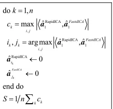
by the computation procedure described in Figure 10.

If , we can regard the two basis sets as having

a similar role. By the computation of S in Figure 10 for

the basis sets of Figures 8 and 9, we found that

0.8

S

0.95

S . Therefore, the basis sets of Figure 8 (Rapid-

ICA) and Figure 9 (FastICA) essentially play the same

role. In other words, both the RapidICA and the FastICA converged to the sound and similar local optimum.

4.3.2. Convergence Comparison by 200 Images: Super-Gaussian Data Set

We prepared a data set of 200 color images as follows.

Figure 8. ICA bases by the RapidICA.

RapidICA

1 1

,

RapidICA

1 1

, RapidICA do 1,

ˆ ˆ max ,

ˆ ˆ , arg max ,

ˆ 0

ˆ 0 end do

1

k

FastICA

k

FastdICA k

i j

FastdICA k k

i j i

j k k

k n c i j

S n c

 



 





a a

a a

[image:9.595.115.231.85.197.2]

a a

Figure 10. Procedure to compute a basis similarity.

As will be seen, the image data are mostly super-Gauss- ian.

Step 1: Each color image was resized to 150 × 112 pixels.

Step 2: From each image, a set of 16,800 patches of 8 × 8 pixels was drawn by overlapped sampling.

Step 3: Each set of patches was normalized to have zero mean.

Step 4: By the whitening method of Equations (15) and (16), the patch vector’s dimension of 192 = 8 × 8 × 3 was reduced to 64.

For the color image data set prepared as described above, we conducted an experiment to compare the RapidICA (Method 3) and the FastICA. The adopted contrast function was log cosh. Figure 11 is a histogram

of the iteration speedup by the RapidICA. Here, the horizontal axis is the speedup ratio, where the truncation criterion of (27) is _104.

necessary iterations for FastICA speedup ratio

necesary iterations for RapidICA

 (34)

The vertical axis is the number of occurrences. Obvi- ously, the RapidICA outperformed the FastICA in all 200 cases. For the total of 200 ICA trials, the RapidICA re- quired 5349 iterations with a CPU time of 1837 seconds by a conventional PC. On the other hand, the FastICA required 9848 iterations with a CPU time of 3031 sec- onds. Therefore, the average iteration speedup ratio was 1.67, and the CPU speedup ratio was 1.65. The most frequent speedup ratio for the iterations was 1.80, and its CPU speedup ratio was 1.78. In all of the 200 cases, the RapidICA outperformed the FastICA.

Accompanied by the 200 image experiments, we used the measure of –log cosh to check the non-Gaussianity. This is illustrated in Figure 12. The horizontal axis is the

non-Gaussianity, and the vertical axis is the number of occurrences. The heavy black arrow is the position of the Gaussian distribution:

 

0.375

J y   (35) As can be understood from Figure 12, the color image

[image:9.595.310.535.86.262.2]

data are super-Gaussian.

[image:9.595.311.536.304.480.2]

Figure 11. Iteration speedup ratio of RapidICA over Fast- ICA on image data.

Figure 12. Non-Gaussianity measure of –log cosh on image data.

4.3.3. Convergence Comparison by 200 EEG Data: Almost Gaussian Data Set

We prepared a data set of 200 EEG vector time series. As will be seen, EEG data are weakly super-Gaussian. That is, they are almost Gaussian, which can cause difficulties in ICA decomposition, as was stated in the ICA formula-tion of Secformula-tion 2.1. The EEG data sets were prepared and preprocessed in the following way:

Step 1: 200 EEG time series were drawn at random from the data of [14]. Each time series had 59 channels.

Step 2: Each EEG time series was divided into chunks that were 8 seconds in length. This generated 8000 sam- ples (1 KHz sampling).

Step 3: Each EEG time series was normalized to have zero mean.

[image:10.595.310.537.85.259.2] [image:10.595.59.285.537.707.2]

Figure 13 illustrates the histogram of the speedup ra-

tio of Equation (34), where the convergence truncation is . For the 200 data sets, the Rapid ICA again outperformed the FastICA in 181 cases. For the total of 200 ICA trials, the RapidICA required a total of 7305 iterations with a CPU time of 613 seconds by a conven- tional PC. On the other hand, the FastICA required 8256 iterations with a CPU time of 656 seconds. Therefore, the iteration speedup was 1.13, and the CPU speedup ratio was 1.07. The most frequent speedup ratio on the itera- tion was 1.30, and its CPU speedup ratio was 1.23. Upon obtaining this result, we checked the degree of the non- Gaussianity.

4

10

_ 

Figure 14 illustrates the non-Gaussianity by using the

measure of –log cosh. The position of the heavy black arrow is that of the Gaussian distribution of Equation (35). As can be observed, sub-Gaussian EEGs were mixed in the test data set. By comparing Figures 12 and 14, one finds that the EEG data drawn from [14] are very

weak super-Gaussian. Some data sets contained multiple Gaussian signals. Such cases violate the assumption of the ICA formulation of Section 2.1. This indicates that appropriate preprocessing is desirable for EEGs before the ICA is applied. We will consider this point in the next section.

5. Concluding Remarks

In this paper, a class of speedy ICA algorithms was pre- sented. This method, called the RapidICA, outperformed the FastICA. Since the increase in computation is very light, the reduction of iterations directly realizes the CPU speedup. The speedup is drastic if the sources are super- Gaussian, which is the case when the source data are natural images. Since ICA bases have the roles of ex- pressing texture information for data compression and measuring the similarity between different images, they

Figure 13. Iteration speedup ratio of RapidICA over Fast- ICA on EEG data.

Figure 14. Non-Gaussianity measure of –log cosh on EEG data with a magnified horizontal axis.

can be used in this system for the similar-image retrieval [7]. In such a case, the speedup of the RapidICA is quite good.

For the case of signals that are nearly Gaussian, such as the EEGs, the RapidICA again outperformed the Fast- ICA in terms of speed. But the margin of improvement is less than that in the case of images. This is because cases of multiple Gaussian sources need to be excluded from the ICA formulation, including both the RapidICA and the FastICA. For such cases, if the ICA is applied, it is necessary to transform raw EEG data into good super- Gaussian data. This is possible on the EEGs since the purpose of using these data in only for the detection of event changes in source signals. This approach will be presented in future papers.

6. Acknowledgements

This study was supported by the Ambient SoC Global COE Program of Waseda University from MEXT Japan. Waseda University Grant for Special Research Projects No. 2010B and the Grant-in-Aid for Scientific Research No. 22656088 are also acknowledged.

REFERENCES

[1] P. Common and C. Jutten, Eds., “Handbook of Blind Source Separation: Independent Component Analysis and Applications,” Academic Press, Oxford, 2010.

[2] A Hyvärinen, “Fast and Robust Fixed-Point Algorithms for Independent Component Analysis,” IEEE

Transac-tions on Neural Networks, Vol. 10, No. 3, 1999, pp. 626-

634.

[3] Y. Matsuyama, N. Katsumata, Y. Suzuki and S. Imahara, “The α-ICA Algorithm,” Proceedings of 2nd

Interna-tional Workshop on ICA and BSS, Helsinki, 2000, pp.

297-302.

Divergence as a Surrogate Function for Independence: The f-Divergence ICA,” Proceedings of 4th International

Workshop on ICA and BSS, Nara, 2003, pp. 173-178.

[5] Y. Matsuyama, N. Katsumata and R. Kawamura, “Inde-pendent Component Analysis Minimizing Convex Di-vergence,” Lecture Notes in Computer Science, No. 2714, 2003, pp. 27-34.

[6] V. Zarzoro, P. Common and M. Kallel, “How Fast Is FastICA?” 14th European Signal Processing Conference

(EUSIPCO), 4-8 September 2006, pp. 4-8.

[7] N. Katsumata and Y. Matsuyama, “Database Retrieval from Similar Images Using ICA and PCA Bases,”

Engi-neering Applications of Artificial Intelligence, Vol. 18,

No. 6, 2005, pp. 705-717. doi:10.1016/j.engappai.2005.01.002

[8] T. Cover and J. Thomas, “Elements of Information The-ory,” John Wiley and Sons, New York, 1991.

doi:10.1002/0471200611

[9] I. Csiszár, “Information-Type Measures of Difference of Probability Distributions and Indirect Observations,”

Studia Scientiarum Mathematicarum Hungarica, Vol. 2,

1967, pp. 299-318.

[10] Y. Matsuyama, “The α-EM Algorithm: Surrogate Likeli-hood Maximization Using α-Logarithmic Information Measures,” IEEE Transactions on Information Theory, Vol. 49, No. 3, 2003, pp. 692-706.

doi:10.1109/TIT.2002.808105

[11] C. M. Bishop, “Neural Networks for Pattern Recogni-tion,” Oxford University Press, Oxford, 1995.

[12] Y. Matsuyama, “Hidden Markov Model Estimation Based on Alpha-EM Algorithm: Discrete and Continuous Alpha-HMMs,” Proceedings of International Joint

Con-ference on Neural Networks, San Jose, 7 July-5 August

2011, pp. 808-816.

[13] H. H. Yang and S. Amari, “Adaptive Online Learning Algorithm for Blind Separation: Maximum Entropy and Minimum Mutual Information,” Neural Computation, Vol. 9, No. 7, 1997, pp. 1457-1482.

doi:10.1162/neco.1997.9.7.1457

[14] B. Blankertz, G. Dornhege, M. Lrauledat, K. R. Muller and G. Curio, “The Non-Invasive Brain-Computer Inter-face: Fast Acquisition of Effective Performance in Un-trained Subjects,” Nueroimage, Vol. 37, No. 2, 2007, pp. 539-550. doi:10.1016/j.neuroimage.2007.01.051

Appendix: R Code of RapidICA

# settings iter.max < − 100 eps < − 1e−5 p.alpha < − 1.0 p.beta < − 1.0 p.gamma < − 1e−6

# initialization W < − diag(1, d, d) dW1 < − matrix(0, d, d) dW2 < − matrix(0, d, d) eta < − matrix(0, d, d)

# iterations

for (p in 1:iter.max) {

# (learning non-gaussianity) Wold < − W

y < − W %*% z dW1 < −

−p.alpha *

diag(1 / rowSums(G2(y))) %*% (G1(y) %*% t(z))

W < − W + dW1 W < − orth(W)

# (convergence test) conv < −

1 − sum(abs(diag(W %*% t(Wold)))) / d if (conv < eps) break

# (acceleration steps) dW2old < − dW2 dW2 < − W − Wold for (i in 1:d) { eta.i.num < −

max(t(dW2[i,]) %*% dW2old[i,], 0) eta.i.den < −

max(t(dW2[i,]) %*% dW2[i,], t(dW2old[i,]) %*% dW2old[i,])

eta[i,i] < − p.beta *

eta.i.num / (eta.i.den + p.gamma) }