The semantics of TLA on the PVS theorem prover

(1)

Original citation:

Wahab, M. (1996) The semantics of TLA on the PVS theorem prover. University of Warwick. Department of Computer Science. (Department of Computer Science Research Report). (Unpublished) CS-RR-317

Permanent WRAP url:

http://wrap.warwick.ac.uk/60998

Copyright and reuse:

The Warwick Research Archive Portal (WRAP) makes this work by researchers of the University of Warwick available open access under the following conditions. Copyright © and all moral rights to the version of the paper presented here belong to the individual author(s) and/or other copyright owners. To the extent reasonable and practicable the material made available in WRAP has been checked for eligibility before being made available.

Copies of full items can be used for personal research or study, educational, or not-for-profit purposes without prior permission or charge. Provided that the authors, title and full bibliographic details are credited, a hyperlink and/or URL is given for the original metadata page and the content is not changed in any way.

A note on versions:

The version presented in WRAP is the published version or, version of record, and may be cited as it appears here.For more information, please contact the WRAP Team at:

(2)

The Semantics of TLA

on the PVS Theorem Prover

M. Wahab

Department of Computer Science

University of Warwick

October 4, 1996

Abstract

An implementation of Lamport’s Temporal Logic of Actions (TLA) on a higher order logic theorem prover is described. TLA is a temporal logic, for which a syntax and semantics are de-fined, based on an action logic which is represented by higher order functions. The temporal logic includes quantifiers for variables with constant values and for variables whose values change over time. The semantics of the latter depend on an auxiliary function which cannot be defined by prim-itive recursion and an alternative is given based on the Hilbertoperator.

1 Introduction

The Temporal Logic of Actions (Lamport, 1994) is a system for reasoning about programs by consid-ering the changes made to program variables during an execution. Actions are boolean expressions relating the values of the variables before and after some event, typically the execution of a command, of the program. Propositional operators are defined on actions giving the base of the temporal logic (the modal system S4.3.1, see Abadi, 1993; Rescher & Urquahart, 1971). This adds the unary operator always,2, such that if2

F

is true at some point during the program execution then

F

is true at that

and every subsequent point. Two existential quantifiers are defined in TLA: the first, over logical vari-ables, has its usual meaning as an abstraction operator which hides a constant value; the second, over variables of the program, hides the values assigned to a variable during the program’s execution. The quantifier free logic is known as Simple TLA and includes a number of nonstandard operators for rea-soning about actions. With a single exception these are derivable from the temporal and propositional operators.

There have been a number of implementations of Simple TLA on theorem provers: TLP (Engberg et al., 1992) uses the first order logic of the Larch prover (Garland & Guttag, 1991) to verify the action logic and a separate verifier for the temporal logic; other implementations used the higher order logic theorem provers HOL (von Wright & L˚angbacka, 1992) and Isabelle/ZF (Kalvala, 1995). Proof rules for TLA have been given by Busch (1995) as axioms for the Lambda theorem prover and for Simple TLA by Engberg (1995) for the TLP prover.

(3)

function can be defined which is equivalent to, and a specification, of the auxiliary function. The se-mantics of the TLA quantifier can then be defined in higher order logic using this specification.

The implementation is given for PVS (Owre, Rushby & Shankar, 1993), an interactive theorem prover based on typed higher order logic with a specification language supporting recursive function and type definitions. Section 2 briefly describes those parts of the specification language used in the implementation. The syntax and semantics of TLA are summarised in section 3 and section 4 describes its implementation on PVS. The implementation uses temporal abstraction to specify the existential quantifier and a proof of the equivalence of the auxiliary function and its specification is given in the

appendix. Section 5 gives an example of how a TLA formula may be presented in the implementation

and is followed by the conclusions.

Notation. Operators: The boolean true, conjunction (and), disjunction (or), negation (not),

impli-cation (implies) and equivalence (iff) operators are, in general and when referring to the PVS logic, given as true,^,_,:,)and,respectively. The symbols8and9denote the universal and

existen-tial quantifiers and appear as e.g. 8(

x

:

T

) :

P

(

x

), where

T

is the type of

x

, or as8

x

:

P

(

x

). The

form

P

[

v=x

]denotes the textual substitution of

v

for free occurrences of

x

in

P

. Functions are given

in lower case or in bold type and predicates end with a question mark; eg and eg are functions and eg? is a predicate. Defined types are usually written with a leading capital although other forms are used when there is no ambiguity.

2 The PVS specification language

A PVS specification is based on modules, called theories, in which types, functions and variables are specified and logical formulae given as axioms or theorems. Functions and types can be passed to modules as arguments and can also be referred to by other modules.

A type is either declared without definition or is defined by enumeration, as an abstract data type or as a subtype by predicates on the values of an existing type. Types provided by PVS include the natural numbers, booleans and infinite sequences of a given type. Tuples have type(

A

1

:::

A

n

)

where each

A

i

is a type which may be distinct from

A

j

(

j

6=

i

). A term of the form

c

:

T

declares the

constant

c

with type

T

.

The definition of an abstract data type (ADT), which may be parameterised, generates a theory containing the definitions and declarations needed for its use. The definition of an ADT has the form

name[

p

1

;:::;p

n

]:datatype begin

cons1(acc1

;:::;

acc

k

):rec1

.. .

cons

m

(acc

1

;:::;

acc

j

):rec

m

end name

The ADT identifier is name, each

p

j

is a parameter to the type, each cons

i

is a constructor and each

acc

l

is an accessor function returning a value of some type. Each rec

i

is a predicate on instances of the ADT acting as a recogniser for the associated constructor, cons

i

, such that rec

i

(

x

)for

x

of type name

is true iff

x

is constructed with cons

i

.

Functions have types(

A

!

B

)and are defined as lambda expressions (and sugared equivalents).

Functions and some operators may be overloaded, e.g. the functions

f

: (nat ! boolean)and

f

:

((natnat) ! nat)are distinct. Predicates are functions returning booleans and sets of a type are

(4)

to show that the function terminates. A limited form of polymorphism is supported: if type

T

is an argument to a theory module, functions can be defined with types dependent on

T

, which will be in-stantiated when the functions are used.

A conditional is provided by anif-then-else-endifexpression for which both branches must be given. An expression for pattern matching on an instance of an ADT is available and is equivalent to a nested conditional using the recognisers of the ADT.

Logical formulae can be presented as axioms, which are assumed to be true, or theorems, which must be proved. A logical formula is any expression which returns a boolean value. The usual op-erators are available and include equivalence, equality and the universal and existential quantifiers. Formulae expressing boolean equivalence can be used by the prover as rewrite rules.

3 TLA

The domain of TLA is the set of states which are modeled as functions from a set of identifiers to a set of values. A program variable, whose value may change, is named with an identifier from the set of identifiers or with an identifier from the set combined with a prime (if

x

is a variable then so is

x

0

). The values of the program variables are given by some state. Rigid (logical) variables have constant values and are independent of the states.

Expressions using program variables are called state functions and their value is dependent on the values of the program variables. A boolean expression in which all program variables are unprimed is a predicate. A primed predicate or function is one in which all program variables are primed: if

P

is a predicate,

P

0

is a primed predicate. A boolean expression which uses both unprimed and primed variables is an action and an expression containing a temporal operator is a temporal formula.

The semantics of the action logic assumes the set of identifiers Vars and the set of values Vals.

Definition 1 States and Behaviours

A state is a total function from Vars to Vals, Stdef

= (Vars!Vals).

A state function is a function which takes a state as an argument and returns an element of some type

T

. The type of state functions is(St!

T

)

A sequence of a type

T

is a total function from the naturals to

T

, Seq[

T

] def

=(nat !

T

) and a

behaviour is a sequence of states, Behaviourdef

= Seq[St]

If

is a behaviour and

n

is a natural then

(

n

)is the

n

th state in the behaviour and

n

is the

behaviour obtained by dropping the first

n

1states in

.

n

def

=(

(

m

:nat):

(

n

+

m

))

The concatenation of a state

s

to the beginning of a behaviour

is written

s

and, for a natural

number

n

, satisfies

(

s

)(

n

)= (

s

if

n

=0

(

n

1) if

n >

0

2

A TLA formula is made up of actions or TLA formulae combined with a logical operators

Definition 2 Formulae of TLA

(5)

(Leads to)

F

;

G

def

= 2(

F

)3

G

)

(Unchanged) Unchanged(

f

) def

=

f

0 =

f

(Stuttering) [

A

]

f

def

=

A

_Unchanged(

f

)

h

A

i

f

def

=

A

^:Unchanged(

f

)

(Fairness) WF

f

(

A

)

def

= 23h

A

i

f

_23:Enabledh

A

i

f

SF

f

(

A

) def

= 23h

A

i

f

_32:Enabledh

A

i

f

where

F

and

G

are temporal formulae,

A

is an action and

f

is a state function.

Figure 1: Derived operators of TLA

The syntax of a TLA formula is

T

::=an actionj:

T

j

T

^

T

j2

T

j9

x

:

T

j9

v

:

T

where

x

is a rigid variable and

v

is an unprimed program variable.

A syntactically correct temporal formula is called a well-formed formula (wff) of TLA. 2

Other logical operators (_,), etc) are derived from the negation and conjunction operators in the

usual way. The dual of the always (2) operator is the eventually operator (3) and3

F

=:2:

F

. The

definitions of the derived TLA operators are given in Figure 1.

The semantics of TLA are given by an interpretation function mapping well-formed formulae and behaviours to booleans.

Definition 3 Semantics of TLA

The interpretation function,I, for action

A

and states

s

and

t

is defined as

I(

A;s;t

) def

=8(

v

:Vars):

A

[

s

(

v

)

=v

][

t

(

v

)

=v

0

](

A

is a boolean expression)

I(Enabled(A)

;s;t

) def

=9(

u

:St):I(

A;s;u

)

For TLA formulae

F

and

G

and behaviour

,Iis defined

I(

F;

) def

= I(

F;

(0)

;

(1))(

F

is an action)

I(:

F;

) def

= :I(

F;

)

I(

F

^

G;

) def

= I(

F;

)^I(

G;

)

I(2

F;

) def

= 8(

n

:nat):I(

F;

n

) I(9

x

:

F;

)

def

= 9(

c

2Vals):I(

F

[

c=x

]

;

)

2

The interpretation function defines the semantics of predicates and primed predicates as instances of actions. For a predicate

P

and states

s

and

t

, the interpretation function givesI(

P;s;t

) = 8(

v

: Vars) :

P

[

s

(

v

)

=v

]andI(

P

0

;s;t

)=8(

v

:Vars):

P

[

t

(

v

)

=v

0

].

(6)

is true in a behaviour

then9

v

:

F

(

v

)is true in any behaviour

which differs from

only in the values

of

v

, since there is a sequence of values which may be assigned to

v

in each state of

to make

F

(

v

)

true in

. The temporal logic is based on actions and

F

(

v

)may depend on the values of variables in

consecutive states. Since

may differ from

only in the value of

v

, this imposes the constraint that for every natural

i

,

(

i

)6=

(

i

+1)iff

(

i

)6=

(

i

+1). This is too strong: when

v

is the only variable

whose value changes, the interpretation of9

v

:

F

(

v

)in

will depend on changes to the value of

v

in

and therefore on the value of

v

. To remove this dependence, only the states of

and

which are not equal to their successors are considered.

Definition 4 Existential quantifier over program variables

An equality,=

v

, between a pair of behaviours, takes a program variable

v

and compares all states

in the behaviours up to

v

.

=

v

def

= 8(

n

:nat):8(

x

2Vars):

x

6=

v

)

(

n

)(

x

)=

(

n

)(

x

)

A reduction function takes a behaviour and removes all states which are equal to their successors.

\

def =

8 > <

> :

if8(

n

:nat):

(

n

)=

(0)

\

1 if

(0)=

(1)

(0)

\

1 if

(0)6=

(1)

For an unprimed program variable

v

, the interpretation of the existential quantifier is defined as

I(9

v

:

F;

) def

= 9(

;

:Behaviour):(

\

=

\

)^(

=

v

)^I(

F;

)

2

4 Implementation of TLA in PVS

Given the sets Vars, of variables, and Vals, of values, the types used in the implementation are as defined for the TLA semantics. TLA formulae are represented by mapping actions to predicates in the PVS logic and by defining the type of well-formed temporal formulae. The semantics of TLA formulae are given by a function from the well-formed formulae to the booleans.

State functions are represented as PVS functions from states to some type

T

. TLA defines opera-tors on state functions and the representation of these operaopera-tors must be defined on functions returning any type. A theory module is declared with type

T

as a parameter and a type tla Fn contains the func-tions from the states to

T

. The representation of the TLA operators are then defined on the tla Fn type: e.g. the representation of the unchanged operator takes an argument of type tla Fn[

T

]and can

be specialised to, among others,

T

=(natnat)and

T

=boolean.

Actions and predicates

Actions are represented as predicates on state pairs.

Definition 5 Type of actions

Actions is the type containing functions from pairs of states to the booleans,

Actionsdef

= ((StSt)!boolean)

(7)

Predicates are state functions of type(St ! boolean) and may be promoted to elements of the

type Actions. The promotion of a predicate

P

to an action is unprimed(

P

)=(

(

s;t

):

P

(

s

))and the

promotion of a primed predicate is primed(

P

)=(

(

s;t

):

P

(

t

)), where

s

and

t

are states.

Temporal Logic

The syntax of the temporal logic is given by an abstract data type, wff, containing the temporal formulae which are either actions or actions composed with a conjunction, negation or always (2) operator. An

interpretation function maps elements of this type to the boolean values, defining the semantics. Because of restrictions on the definition of abstract data types, the existential quantifiers cannot be defined directly but are described as predicates on behaviours. The syntax and semantics of the quantifiers are then defined by the parameters and definitions of these predicates.

Definition 6 Type of temporal formulae

The abstract data type wff has the base constructors action, on actions, and exf, on predicates over behaviours. It has the recursive constructors not, and and2representing temporal formulae with

nega-tion, conjunction and always.

wff:datatype

begin

action (ac:Actions) :action?

not (neg:wff) :not?

and (lcj:wff

;

rcj:wff) :and?

always (alw:wff) :always?

exf (exw:(Behaviour!boolean)) :exf? endwff

A temporal formulae has the type tla Formula, and its subtype, act Formula, contains only for-mulae representing actions.

tla Formuladef = wff act Formuladef

= f

F

:tla Formulajaction?(

F

)g

2

Operators are written using infix notation, e.g. and(A, B) is given as

A

and

B

; the formula

always(

F

)is written as2

F

.

The semantics of the temporal formulae are defined by the interpretation function, trans, mapping an element of type tla Formula and a behaviour to the boolean values.

Definition 7 Interpretation of temporal formulae

The function trans has the type trans:((tla FormulaBehaviour)!boolean)and is recursively

defined as

trans(action(

A

)

;

) def

=

A

(

(0)

;

(1))

trans(not(

F

)

;

) def

= :trans(

F

)

trans(and(

F;G

)

;

) def

= trans(

F;

)^trans(

G;

)

trans(2

F

)

;

) def

= 8(

n

:nat):trans(

F;

n

)

trans(exf(F)

;

) def

= F(

)

(8)

(Enabled) enabled(

A

) :act Formula def

= action(unprimed(

s

:(9

t

:

A

(

s;t

))))

(Unchanged) unchanged(

f

) :act Formula def

= action(

(

s;t

):

f

(

t

)=

f

(

s

))

(Eventually) 3

F

:tla Formula

def

= not2not

F

(Leads to) ;(

F;G

) :tla Formula

def

= 2(

F

implies3

G

)

(Stuttering) square(

A;f

) :tla Formula def

= (

A

&action(

(

s;t

):

f

(

t

)=

f

(

s

)))

angle(

A;f

= (

A

j action(

(

s;t

):

f

(

t

)=

f

(

s

)))

(Fairness) WF(

A;f

) :tla Formula

def

= 23(angle(

A;f

))

or23not(enabled(angle(

A;f

)))

SF(

A;f

= 23(angle(

A;f

))

or32not(enabled(angle(

A;f

)))

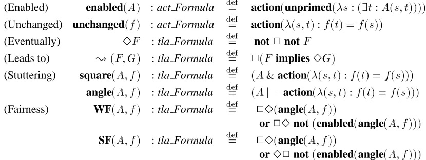
[image:8.595.92.507.123.279.2]

where

f

:tla Fn,

A

:act Formula and

F;G

:tla Formula.

Figure 2: TLA derived operators

The boolean true is defined as an instance of the actions subtype, act Formula. Negation and con-junction operators are also defined for the act Formula subtype and are named to avoid ambiguity with the operators of the temporal formulae.

Definition 8 Action operators

The boolean true is the action which returns true for all states. The negation ( ) and conjunction (&) operators on action formulae create new instances of the act Formula subtype.

true :act Formula def

= action(

(

s;t

:St):true) (

A

) :(act Formula!act Formula)

def

= action(

(

s;t

:St)::ac(

A

)(

s;t

))

&(

A;B

) :((act Formulaact Formula)!act Formula) def

= action(

(

s;t

:St):ac(

A

)(

s;t

)^ac(

B

)(

s;t

))

The disjunction (j) operator on actions is derived from the negation and conjunction operators. 2

An action operator applied to formulae of type act Formula will return an action formula (of type

act Formula) and a temporal logic operator will return a temporal formula (of type tla Formula).

Def-initions of the nonstandard operators are given in Figure 2.

The quantifier for rigid variables is represented as a higher order function, existc, constructing a TLA formula with the exf form.

Definition 9 Quantification over rigid variables

The existential operator for rigid variables takes a function from a value to a TLA formula and returns a well-formed formula.

existc(

H

) :((Vals!tla Formula)!tla Formula) def

= exf(

:9(

c

:Vals):trans(

H

(

c

)

;

))

(9)

The definition of the function trans gives the existential quantifier for rigid variables the interpre-tation trans(existc(

H

)

;

)=(9(

c

:Vals) :trans(

H

(

c

)

;

)).

Existential quantification over program variables

The reduction function on behaviours,

\

, cannot be defined by primitive recursion: if the behaviour

satisfies8

i

:9

j

:

i

(0)6=

i

(

j

)then

\

never terminates. Instead, a function, stut, which specifies

\

is used in the definition of the quantifier.

The definition of stut is based on the indices of the state changes in a behaviour

where

i

is the index of a state change iff

(

i

)6=

(

i

+1). The first state change in a behaviour is the least index and

is specified using a description operator (

). The

n

th state change,

n >

0, is found by dropping the

prefix of

up to and including the(

n

1)th state change.

The epsilon operator,

, returns any element of a given set; if the set is empty,

returns any value. The function choose applies the epsilon operator to a given nonempty set1. The PVS types set[

T

]and nonempty?[

T

]define the sets of type

T

and nonempty sets of type

T

respectively.

Definition 10 Choice

The choice function choose takes a nonempty set

S

and returns some element of

S

.

choose:(nonempty?[

T

]!

T

) def

=

(

S

)

where

(

S

)2

S

2

For a behaviour

, the set

I

(

)contains the naturals which are indices of state changes in

. The

first state change in

is contained in the, singleton, subset of

I

(

)given by least(

I

(

)).

Definition 11 Indices of state changes

The function

I

takes a behaviour

and returns the set of naturals such that

i

2

I

(

) ,

(

i

) 6=

(

i

+1).

I

:(Behaviour!set[nat])

I

(

)

def

=f

i

:natj

(

i

)6=

(

i

+1)g

Given a set of naturals, least returns the subset containing the least element of the set.

least :(set[nat]!set[nat])

least(

S

) def

= f

i

j

i

2

S

^:(9

j

:

j

2

S

^

j < i

)g

2

If a behaviour

has any state change, the index of the first is given by choose(least(

I

(

)))since choose returns any element of the (singleton) set least(

I

(

)).

A behaviour which contains no state changes is said to be empty.

Definition 12 Empty behaviours

A behaviour is empty if every state in the behaviour is equal to the first state.

empty?(

),8

n

:

(

n

)=

(0)

2

1_The

(10)

Corollary 1 For any behaviour

, empty?(

),

I

(

)=fg

Proof. empty?(

) )

I

(

) = fg: For every natural,

i

,

(

i

)=

(0) =

(

i

+1)and

I

(

)is empty.

I

(

)=fg)empty?(

): There is no index

i

of

such that

(

i

)6=

(

i

)and empty?(

)follows. 2

The index of the

n

th state change in a behaviour

is the index of the first state change after drop-ping the prefix of

up-to and including the(

n

1)th state change. This gives an index relative to the

(

n

1)th state change and the number of states in the prefix must be added to get the actual index.

Definition 13 Index of a state change in a behaviour

The function next takes a behaviour

and a natural

n

and returns the index of the

n

th state change in

.

next :((Behaviournat)!nat)

next(

;n

) def

= 8 > <

> :

0 if empty?(

)

choose(least(

I

(

))) if

n

=0 next(

;n

1)+1+next(

;

0) otherwise

2

The function next terminates since the number of self-references is bounded by the argument

n

. The function stut, on a behaviour

returns a behaviour

constructed from the states of

which differ from their successor and satisfying

(

n

)=

(next(

;n

)).

Definition 14 Reduction function

The function stut specifies the reduction function on behaviours.

stut :(Behaviour!Behaviour)

stut(

) def

=(

(

n

:nat):

(next(

;n

)))

2

The function stut is equivalent to the TLA behaviour reduction function.

Theorem 1 For any behaviour

, stut(

)=

\

.

Proof. The proof is given in Appendix A and is by extensionality and induction with three main steps:

1. a proof that stut(

)(0)=

\

(0),

2. a proof that(

\

)

n

=

\

(

n

)written as

(next(

;n

))and

\

(

n

)as(

\

)

n

(0), using the results of (1) and (2)

to show that

(next(

;n

))=

\

(

(next(

;n

)))(0).

2

(11)

Definition 15 Existential quantifier

The function equals? has type((Vars!(BehaviourBehaviour))!boolean)and is defined as

equals?(

v

)(

;

) def

= (8(

w

:Vars):(8(

n

:nat):

w

6=

v

)

(

n

)(

w

)=

(

n

)(

w

)))

The existential operator on program variables, existv, takes a variable and a function from the vari-ables to the TLA formulae and returns a well formed formula.

existv(

v;F

):((Vars(Vars!tla Formula)!tla Formula)) def

= exf(

:(9(

;

:Behaviour): stut(

)=stut(

)^equals?(

v

)(

;

) ^trans(

F

(

v

)

;

)))

2

5 Example

A simple example of the representation of a TLA formula is taken from Lamport (1994). A TLA for-mula specifies a program with two integer variables which are both initially0and whose values

increase in steps.

initdef

= (

x

=0)^(

y

=0)

M

1

def = (

x

0

=

x

+1)^(

y

0

=

y

)

M

2

def = (

y

0

=

y

+1)^(

x

0

=

x

)

M

def

=

M

1

_

M

2

def

= init ^2[

M

] (

x;y

)

^WF (

x;y

)

(

M

1

)^WF (

x;y

)

(

M

2

)

init is a predicate,

M

1

;M

2and

M

are actions and

is a temporal formula. The identifiers and

values are defined as types.

Vars:type=f

x;y

g Vals:type=int

The predicate init contains only unprimed variables and is translated to a predicate on a state. It is defined as a lambda expression taking a state

s

and each occurrence of

x

and

y

in init is replaced with

s

(

x

)and

s

(

y

)respectively. The action constructor returns an action formula.

init:act Formula def

= action(unprimed(

(

s

:St) :(

s

(

x

)=0)^(

s

(

y

)=0)))

The actions

M

1and

M

2 are represented in the same way: they are defined as lambda expressions

taking a pair of states,

s

and

t

; each unprimed variable

v

is replaced by

s

(

v

)and each primed variable

v

0

is replaced by

t

(

v

).

m1

:act Formula def

= action(

(

s;t

:St):(

t

(

x

)=(

s

(

x

)+1))^(

t

(

y

)=

s

(

y

)))

m2

:act Formula def

= action(

(

s;t

:St):(

t

(

y

)=(

s

(

y

)+1))^(

t

(

x

)=

s

(

x

)))

The action

M

is a disjunction of actions and can be translated as the disjunction of either temporal or action formulae. The first gives an instance of the TLA formulae type and disallows the use of m where an action is required. The second returns an action which may be used in both temporal and action formulae.

m:act Formula def

= m 1

(12)

The formulahas terms which take a tuple of the program variables,(

x;y

), as an argument. The

value of the tuple is given by the value of the variables in a particular state and the tuple can be consid-ered a function taking variables and returning a state function. The two-place tuple is defined to take a PVS tuple of variables and returns a function from a state to a PVS tuple of values.

tuple(

a;b

) :((VarsVars)!(St!(ValsVals))) def

= (

(

s

:

State

) :(

s

(

a

)

;s

(

b

)))

The TLA formulais translated as

Phi:tla Formula def

= init and square(m

;

tuple(

x;y

))

and WF(m 1

;

tuple

(

x;y

))and WF(m 2

;

tuple

(

x;y

))

This combines the actions and predicates using the propositional operators defined on the type

tla Formula to return an element of type tla Formula.

6 Conclusion

The model used in the implementation follows that of the TLA report (Lamport, 1994) and is based on infinite sequences of states in which the semantics of the operators are defined. The use of infinite sequences to represent behaviours means that the TLA function for reducing stuttering behaviours,

\

cannot be given directly. Instead, a function stut is defined which specifies, and is equivalent to, the reduction function. It is this specification function which is used in the definition of the existential quantifier. The model is similar to that used by von Wright & L˚angbacka for the implementation on HOL, in which the states are represented as tuples of values and the behaviours as sequences of state. In the implementation for Isabelle (Kalvala, 1995), a behaviour is represented as a list of the changes made to states with the empty list representing the behaviour in which there are no state changes.

The formulae of TLA are defined as instances of a type of well-formed formula, as the subset of this type containing only the actions and as the PVS representation of actions. These simplify the definition of the TLA syntax since only a small number of basic operators are needed. The separation of tem-poral and action formulae is common in other implementations: in the HOL implementation of TLA, actions are lambda expressions on tuples of values and temporal formulae are lambda expressions on behaviours. In the Isabelle implementation, actions are predicates on states, the syntax of TLA is de-fined as an abstract data type and the interpretation of a TLA formulae is as a predicate on behaviours. In both of these implementations, separate operators are defined for action and temporal formulae.

References

Abadi, M. (1993). An axiomatisation of Lamport’s temporal logic of actions. Technical Report 65, DEC Systems Research Center.

Busch, H. (1995). A practical method for reasoning about distributed systems in a theorem prover. In Schubert, E. T. et al. (Eds.), HUG ’95, Volume 971 of Lecture Notes in Computer Science. Springer-Verlag.

(13)

Engberg, U., Grønning, P. and Lamport, L. (1992). Mechanical verification of concurrent systems with TLA. In von Bochmann, G. and Probst, D. K. (Eds.), Proceeding of the 4th International

Workshop on Computer Aided Verification, Volume 663 of Lecture Notes in Computer Science.

Springer-Verlag.

Garland, S. J. and Guttag, J. V. (1991). A guide to LP, the Larch Prover. Technical Report 82, DEC Systems Research Center.

Kalvala, S. (1995). A formulation of TLA in Isabelle. Available from the Computer Laboratory, University of Cambridge.

Lamport, L. (1994, may). The Temporal Logic of Actions. ACM Transactions on Programming

Languages and Systems 16(3), 872–923.

L˚angbacka, T. (1994). A HOL formalisation of the Temporal Logic of Actions. In Melham, T. F. and Camilleri, J. (Eds.), Higher Order Logic Theorem Proving and Its Applications, Volume 859 of

Lecture Notes in Computer Science, pp. 332–354. Springer-Verlag.

Melham, T. F. (1993). Higher Order Logic and Hardware Verification. Cambridge Tracts in Theo-retical Computer Science. Cambridge University.

Owre, S., Rushby, J. M. and Shankar, N. (1993). PVS: A Prototype Verification System. Technical Report SRI-CSL-93-04, SRI.

Rescher, N. and Urquahart, A. (1971). Temporal Logic. Library of Exact Philosophy. Springer-Verlag/Wien.

von Wright, J. and L˚angbacka, T. (1992). Using a theorem prover for reasoning about concurrent algorithms. In CAV ’92, Volume 663 of Lecture Notes in Computer Science. Springer-Verlag.

A

Stuttering Behaviours

The proof was carried out using the PVS proof checker with the definition of the function

\

given as an axiom and used as a rewrite rule.

Two properties of the suffix function are used: for any behaviour

and naturals

n

and

m

,

(

n

+

m

) =

(

n

)

m

and

n

(0)=

(

n

). Both can be proved from the definition of the suffix.

A.1 Properties of choose and next

For a nonempty behaviour,

, any member of the set returned by least(

I

(

))is the index of the first

state change of

.

Lemma 1 Properties of choose: I

For any behaviour

which is not empty,:empty?(

),

8

n

:

n <

choose(least(

I

(

))))

(

n

)=

(

n

1)

Proof. Since:empty?(

),

I

(

)is not empty and there is a unique natural

i

2

I

(

)which is less than

any other member of

I

(

). From the definitions, least(

I

(

))=f

i

gand choose(f

i

g)=

f

i

g=

i

and

(

i

) 6=

(

i

+1). Since

i

2 least(

I

(

))it follows that8

n

:

n < i

)

(

n

) =

(

n

+1)(otherwise

n

2

I

(

)contradicting

i

2least(

I

(

))). 2

(14)

Lemma 2 Properties of choose: II

For any behaviour

which is not empty,:empty?(

),

8

i

:

i

choose(least(

I

(

))))

\

(

i

)=

\

(

)

Proof. The proof uses the formula

8

i <

choose(least(

I

(

))):

\

(

i

)=

\

(

i

+1

) (1)

Proof of Formula 1:

Since

i <

choose(least(

I

(

)))and least(

I

(

))is a singleton set,

i

62least(

I

(

))and

i

62

I

(

)giving

(

i

)=

(

i

+1)and

i

(0)=

i

(1). By definition

\

(

i

)=

\

(

i

+1 ).

Proof of Lemma 2: By induction on

i

choose(least(

I

(

))).

Case

i

=0:

\

(

0

)=

\

(

0

)is trivially true. Case

i >

0and

\

(

0

) =

\

(

i

1)

): From Formula 1,

\

(

i

1

) =

\

(

i

) and from the assumption,

\

(

0

)=

\

(

i

). 2

For any nonempty behaviour

, the state indexed by next(

;

0)differs from its successor.

Lemma 3 Properties of next

For any behaviour

which is not empty,

(next(

;

0))6=

(next(

;

0)+1)

Proof. From the assumption that

is not empty and from the definition of next,

next(

;

0)=choose(least(

I

(

)))

From the epsilon axiom,

choose(least(

I

(

)))2least(

I

(

))

) choose(least(

I

(

)))2

I

(

) (definition of least) )

(choose(least(

I

(

))))6=

(choose(least(

I

(

)))+1) (definition of

I

)

(next(

;

0))6=

(next(

;

0)+1) (definition of next)

2

A.2 Equivalence of stut

()

and

\()

For empty behaviours the proof is immediate.

Lemma 4 Equivalence for empty behaviours

For any empty behaviour

, stut(

)and

\

are equivalent.

empty?(

))8

n

:stut(

)(

n

)=

\

(

n

)

Proof. The definition of

\

gives

\

=

and

\

(

n

)=

(

n

). The definition of next gives next(

;n

)=0

and stut(

)(

n

)=

(next(

;n

))=

(0). From the definition of empty?(

),8

n

:

(

n

)=

(0).

(15)

The proof of equivalence for nonempty behaviours uses the fact that the behaviours stut(

)and

\

have the same first state.

Theorem 2 Base case

For any behaviour

, stut(

)(0)=

\

(0)

Proof. The case when

is empty is proved by Lemma 4.

Assuming

is not empty, the definition of stut gives

(next(

;

0))=

\

(0)and from the definition of next,

next(

;

I

(

)))

)

\

=

\

(

;

0))6=

(next(

;

0)+1) (Lemma 3) )

\

(

;

0)) (definition of

\

)

2

The proof of the general case is based on the the equivalence(

\

)

n

=

\

(

n

th state and the reduction of the suffix starting at the

n

+1th state change.

Lemma 5 For any behaviour

,

\

(

\

(

(next(

;n

)+1) )

Proof. With

N

=next(

;n

), the definition of next gives

next(

;n

+1)=(

N

+1)+next(

(

N

+1)

;

0)

Case empty?(

N

): If

N

is is empty then so is

(

N

+1)and next

(

;n

+1)= (

N

+1). Substituting

for

N

gives next(

;n

+1)=next(

;n

)+1and

\

(

\

(

;

0) = 0 and next(

;n

+1) = (

N

+1). Substituting for

N

gives next(

;n

+1) = next(

;n

)+1and

\

(

\

(

;n

+1)=(

N

+1)+next(

;

0)

which gives

\

=

\

(

((

N

+1)+next(

;

0)) )

)

\

((

(

N

+1)

)next (

;

0)

)=

\

(

\

(

\

(:empty?(

), definition of next and Lemma 2)

Substituting for

and

N

gives,

\

(

(next(

;n

)+1)

) =

\

(

(next(

;n

)+1+next(

;

0)) ) =

\

(

(next(

;n

)+1+next(

(next(;n)+1)

;

0))

)

=

\

(

n

,

(

\

)

n

=

\

(

;n

)=0,

\

(

0

)=

0and

(

\

)

n

=

n

. By extensionality,

0

=

n

.

Assuming that

is not empty, the proof is by induction on

n

.

Case

n

=0: From the definition of next(

;

0)and Lemma 2,(

\

)=

\

(

n >

0and assuming(

\

)

(

n

1)

=

\

(

N

=next(

;n

1)and

=

(next(

;n

1)+1)the definition of next gives next(

;n

)=(

N

+1)+next(

(

N

+1)

;

0)

The value of next(

;n

)depends on whether

N

is empty.

Case empty?(

N

): If

N

is empty then so is every suffix of

N

including

(

N

+1).

\

(

N

+1) )=

(

N

+1) )

\

(

(next(

;n

1)+1)

)=

N

) )

\

(

\

)

n

1

=

\

(

\

(

next (

;n

1)

)=

next

(

;n

1) (

N

is empty and

N

=next(

;n

1))

\

)

n

=(

\

)

n

=

next

(

;n

1)+1 (property of suffixes) Case:empty?(

N

): From the property of suffixes,

(

\

)

n

=((

\

) (

n

1)

) 1 ) (

\

)

n

=(

\

(

N

))

1 (inductive hypothesis)

) (

\

)

n

=(

\

(

N

)

By extensionality, for any natural

c

,

(

\

)

n

(

c

)=(

\

(

N

)) 1

(

c

)

) (

\

)

n

(

c

)=

\

(

N

)(

c

+1) (definition of suffix)

N

(0)6=

N

(1) (Lemma 3)

) (

\

)

n

(

c

)=

\

(

N

+1

)(

c

) (definition of

\

) ) (

\

)

n

(

c

)=

\

(

c

) (replacing

N

)

) (

\

)

n

(

c

)=

\

(

c

) (Lemma 5)

) (

\

)

n

=

\

(

\

.

Proof. By extensionality, for any natural

n

, stut(

)(

n

)=

\

(

n

). If

n

=0, the equivalence is proved

by Theorem 2. Assume that

n >

0.

By definition,

stut(

)(

n

) =

(next(

;n

))

=

\

(

n

) =(

\

)

n

(0) =

\

(

;

0)) (definition of stut)

The equivalence to be proved is therefore

next(

;n

)

(0)=

next (

;n

)

(next(

next (

;n

)

;

0))

By definition, next(

;n

)=next(

;n

1)+1+next(

(next(

;n

1)+1)

;

0). With

=

(next(

;n

1)+1),

the proof is by cases of empty?(

).

Case empty?(

(next(

;n

1)+1) ):

From the definition of next,

next(

(next(

;n

1)+1)

;

0)=0 (definition of next)

) next(

;n

)=(next(

;n

1)+1) )

;

0))

=

;

0)) =

\

(

n

)=

;

0)), the proof is by showing next(

;

0)=0.

The definition of next gives

next(

;

0) =next(

(next(

;n

1)+1+next(

;

0))

;

0) (

=

;

0) (writing with a suffix)

Writing this with

gives

next(

next (

;n

)

;

0)=next(

next (

;

0)

;

(18)

is not empty and from Lemma 3,

(next(

;

0))6=

(next(

;

0)+1).

(next(

;

0))=

;

0)+1)=

next (

;

0)

(1)

) next(

;

0)2

I

(

I

)

and 02least(

I

(

;

I

(

next (

;

0)

))) (definition of next) ) next(

;

0)=0

) next(

;

0)=0 (Formula 2)

;

0))is therefore

\

(

n

)=

n

)

completing the proof.