Application of Eigenfunction Orthogonalities to Vibration Problems

Abstract— The modelling of vibration problems is of great importance in engineering. A popular method of analysing such problems is the variational method. The simplest vibration model is represented using the example of a long rod. Two kinds of eigenfunctions orthogonality are proved and the corresponding norms are used to derive Green's function that gives rise to an analytical solution of the problem. The method can be easily generalized to a broad class of hyperbolic problems.

Index Terms— Bishop-equation, Green’s function, Orthogonality, wave equation.

I. INTRODUCTION

The longitudinal vibration of a thin isotropic bar has been studied by many researchers over a long time owing to its wide applications in engineering. More specifically, the vibration in a thin bar is described by PDE of the second order (E.g.: wave equation) and the vibration in a thick bar is described by PDE of the forth or higher order (E.g. Rayleyh, Rayleigh-Bishop Equations etc.) [1], [2], [3], [4]. There are many ways of modelling vibration problems. In our opinion, the best method of such modelling is the variational principle [5]. The following reasons show the advantage of this method.

• Simultaneously with the differential equation we can obtain necessary boundary conditions.

• Using the method of separation of variables (when it is available), and different kinds of orthogonality (method of multiple orthogonalities), we can obtain very simple form of Lagrangian.

• This allows, (and this is the main idea of the paper), to construct Green's function of the problem that is equivalent to obtaining an analytical solution. For the sake of simplicity in this paper we demonstrate the method of two orthogonalities using a simple example of the wave equation. To be more precise we consider the forced vibration analysis of a thin homogeneous bar with constant

Manuscript received April 14, 2009

a_{Department of Mathematics and Statistics, Tshwane University of}

Technology, P .O. Box X680, Pretoria, 0001 FIN-40014, South Africa. phone: +27123826416; fax: +27123826114; e-mail: fedotovi@tut.ac.za (corresponding author), DjouosseuTenkamHM@tut.ac.za).

b_{School of Chemical and Metallurgical Engineering, University of}

Witwatersrand, P.O. Box. 3 Wits, Johannesburg, 2050, South Africa e-mail: Tatiana.Fedotova@wits.ac.za

c_{Manufacturing and Materials Sciences, Council for science and}

Industrial research (CSIR), P.O. Box 395, Pretoria 0001, South Africa e-mail: mshatlov@csir.co.za

cross-section, assuming that both ends of the bar are suspended by lumped masses and springs. This leads to the well known second order wave equation with constant coefficients with the natural homogeneous boundary conditions of the third kind. This example is considered in detail.

The transcendental equation determining the corresponding eigenvalues is solved using different mathematical software. The corresponding eigenfunctions satisfy two kinds of orthogonality conditions. The results are checked by means of MathCAD. The Green function is directly derived in terms of eigenfunctions and also used to obtain the solution of the problem.

This method can be easily generalized for equations of higher order describing the vibration in thick bar with variable geometry. The analytical tools of such generalization are based on finding eigenfunctions with piecewise continuous derivatives.

II. GOVERNING EQUATION AND BOUNDARY CONDITIONS

Let us consider a homogeneous isotropic thin bar of length 1. We suppose that the small vibrations are activated by the distributed force

F

=

F

(

x

,

t

)

. In such condition the mechanical wave displacement that comes from the deformation of the medium is represented by

u

=

u x t

( )

,

where

x

and

t

are respectively the axial distance between the points along the bar and the time. The Lagrangian, is the difference of its kinetic energy, its combined potential energies due to the strain in the bar and due to the elasticity of the surrounding medium at the ends of the bar in which the motion took place and the work done by the external applied force [5].

(

)

[

]

[

]

∫

∫

−

+

−

−

+

′

−

=

′

1

0

2 2

0 1

0

2 2

(1)

)

1

(

)

(

2

1

2

2

1

,

,

dx

u

x

u

x

dx

Fu

u

E

u

A

u

u

u

L

l

δ

β

δ

β

ρ

where

A

=

A

(

x

)

is the cross-section area,

ρ

is the mass density,

E

is Young modulus of elasticity,

β

₀ and

β

_l are the elasticity constant at both ends of the bar,

δ

(

x

)

is the Dirac

δ

−

function with support at

x

=

0

and the upper dot and the prime denote respectively the derivative with respect to

t

and

x

. In accordance with the Hamiltonian principle

Application of Eigenfunction Orthogonalities to

Vibration Problems

the variation of the action

=

∫

2

1

t t

Ldt

S

must be equal to zero for all

t

₁and

t

₂. [5]. Thus

∫

=

=

2 1

0

t t

Ldt

S

δ

δ

(2)

(It is necessary to distinguish two notations:

δ

(

x

)

(with brackets) - Dirac

δ

−

function and δ (without brackets) - variation of functional or function).

It is easy to see (assuming

δ

u

(

x

,

t

₁

)

=

δ

u

(

x

,

t

₂

)

=

0

)

(

)

(

)

[

]

[

]

2 1

2 1

2 1

1

0

0

(1, ) (1, ) (1, )

(0, ) (0, ) (0, ) 0 (3)

t t t

l t

t t

S EAu Au FA udxdt

x t

EAu t u t u t dt

EAu t u t u t dt

δ

ρ

δ

β

δ

β

δ

∂ ∂

⎡ _′ ⎤

= _⎢ − + _⎥ +

∂ ∂

⎣ ⎦

′

+ − +

′

− + =

∫ ∫

∫

∫

Equation (3) is satisfied if

(

Au

)

(

EAu

)

FA

(4)

t

ρ

x

∂

₋

∂

_′

₌

∂

∂

(equation of motion) and boundary conditions

0

)

,

1

(

)

,

1

(

0

)

,

0

(

)

,

0

(

1 0

=

+

′

=

−

′

t

u

t

u

t

u

t

u

α

α

(5)

are of the third kind) where

α

₀

=

β

₀

/

EA

and 1 1

EA

β

α

=

.

The initial conditions are given as follows:

( ) ( )

x

,

0

g

x

and

u

( ) ( )

x

,

0

h

x

.

u

=

=

(6)

Remark: We consider boundary conditions of the third kind because they produce nonconventional orthogonality conditions (the second orthogonality). These conditions are given below (formula (17)).

III. FREE VIBRATION AND STURM-LIOUVILLE PROBLEM

Let us suppose that

A

,

E

,

ρ

are constants. Problem (4)-(5) becomes of the following form:

F

x

u

E

t

u

₌

∂

∂

−

∂

∂

2 2

2 2

ρ

(7)

With the boundary conditions:

0

)

,

1

(

)

,

1

(

0

)

,

0

(

)

,

0

(

1 0

=

+

′

=

−

′

t

u

t

u

t

u

t

u

α

α

. (8) To state the Sturm-Liouville problem, we set

F

(

x

,

t

)

=

0

. The classical Fourier method consists in setting

( ) ( )

i t

e

x

y

t

x

u

,

=

ω (9) where 2

₌

₋

1

.

i

Substituting expression (9) into equation (7), (8) leads to the Sturm-Liouville problem:

( )

( )

( )

( )

( )

( )

⎪

⎭

⎪

⎬

⎫

=

+

′

=

−

′

=

+

′′

0

1

1

0

0

0

0

1 0 2

y

y

y

y

x

y

x

y

α

α

λ

(10)

where

( )

ρ

ω

ω

λ

λ

c

E

c

=

=

=

and

is the velocity in the

bar. The general solution of equation (7) has the following form:

( )

x

a

x

b

x

y

=

sin

λ

+

cos

λ

(11) where

a

and

b

are constant which can not be simultaneously equal to zero. Substituting (11) into boundary conditions in (10) gives the following characteristic equation with

λ

as unknown:

( )

(

2

)

sin

(

_{0 1}

)

cos

0

.

(12)

1

0

+

+

+

=

=

α

α

λ

λ

λ

α

α

λ

λ

D

Many positive roots

λ

n

,

n

=

1

,

2

,...

, of the transcendental

equation (12) can be obtained by using mathematical software such as Mathcad (more on that in the numerical discussion). The corresponding eigenfunctions are

( )

x

a

sin

x

b

cos

x

.

y

y

_n

=

_n

=

_n

λ

_n

+

_n

λ

_n

IV. THE ORTHOGONALITY OF THE EIGENFUNCTIONS

Let

y

n

and

y

mbe the two distinct eigenfunctions (

n

≠

m

) corresponding to the different eigenvalues

λ

n

and

λ

mthat is

0

2

₌

+

′′

_{j j}

j

y

y

λ

(13)

( )

( )

( )

1

( )

1

0

0

0

0

1 0

=

+

′

=

−

′

j j

j j

y

y

y

y

α

α

(14) where

j

=

m

,

n

(,

n

≠

m

)

The standard orthogonality of eigenfunctions is usually obtained by multiplication of equation for

y

_n by

y

_m , equation for

y

_mby

y

_n integration with respect to

x

from 0 to 1 and subtraction of results obtained. Consequently,

( ) ( )

₁2

,

1

0

y

m

x

y

n

x

dx

=

y

n

δ

nm

∫

(15)

where

( )

x

dx

y

y

n n

=

∫

1

0 2 2

1 (16) and

δ

_nm is Kronecker’s symbol.

In order to obtain the second orthogonality, we repeat the above technique but by multiplying equations for

y

nand

m

y

by

λ

_m2

y

_m

and

λ

_n2

y

_n respectively and by using the

boundary conditions

( )

0

_{0 n}

( ) ( )

0

,

_n

1

_{1 n}

( )

1

and

_m

( )

0

_{0 m}

( )

0

,

n

y

y

y

y

y

y

′

=

α

′

=

−

α

′

=

α

( )

1

_{1 m}

( )

1

.

m

y

y

′

=

−

α

This yields the second boundary condition:

1

0 1

0 2 2

( ) ( )

(0)

(0)

(1)

(1)

(17)

m n n m n m

n nm

y

x y x dx

y

y

y

y

y

α

α

δ

′

′

+

+

=

∫

where

).

1

(

)

0

(

)

(

2

1 2

0 1

0 2 2

2

y

x

dx

y

n

y

n

In the case α_₀ =

α

₁ =0 orthogonality (17) is given in [6], (page 382). In the case of processes described by the wave equation this orthogonality is obvious. For more sophisticated PDE of higher order we present below a more complicated kind of the second orthogonality, but this one appears to have never been used before for determining of solutions in terms of Green’s function.

V. SOLUTION OF THE PROBLEM

We seek the solution of problem (7), (8), (6) in the form of a generalised Fourier series with respect to the eigenfunctions of the Sturm-Liouville problem:

( ) ( )

t

y

x

u

t

x

u

_n n n

∑

∞ =

=

1

)

,

(

(19)

where

u

_n

( )

t

is an unknown function. We can also expand the right hand side

F

with respect to the same eigenfunctions system:

( )

_∑

∞

( ) ( )

=

=

1

,

n n n

t

y

x

F

t

x

F

(20)

where

F

_n

(

t

)

is

n

-th Fourier coefficient of

F

:

( )

F

( ) ( )

x

t

y

x

dx

y

t

F

_n

n

n

=

∫

1 0 2 1

,

1

(21) In order to obtain the equation for the determination of

( )

t

u

_n , the Euler-Lagrange differential equation is used:

0

=

∂

∂

−

⎟

⎠

⎞

⎜

⎝

⎛

∂

∂

u

L

u

L

dt

d

(22)

where

L

is Lagrangian (1) defined above.

Substituting (19) and (20) into Lagrangian (1) after simple transformation we obtain:

(

)

(23)

)

(

)

(

)

1

(

)

1

(

2

1

)

(

)

(

)

0

(

)

0

(

2

1

)

(

)

(

)

(

)

(

2

1

)

(

)

(

)

(

)

(

)

(

)

(

)

(

)

(

2

1

,

,

1 1 1 1 0 1 1 0 1 0 1 1 1 0 1 1 1 0 1 0 1 1

dx

t

u

t

u

y

y

E

A

dx

t

u

t

u

y

y

E

A

dx

t

u

t

u

x

y

x

y

E

A

dx

x

y

x

y

t

u

t

F

A

dx

t

u

t

u

x

y

x

y

A

u

u

u

L

n m m n m n n m m n m n n m m n m n n m m n n m n m m n m n

⎟

⎠

⎞

⎜

⎝

⎛

−

−

⎟

⎠

⎞

⎜

⎝

⎛

−

−

⎟

⎠

⎞

⎜

⎝

⎛

_′

_′

+

+

⎟

⎠

⎞

⎜

⎝

⎛

+

+

⎟

⎠

⎞

⎜

⎝

⎛

=

′

∑∑

∫

∑∑

∫

∑∑

∫

∑∑

∫

∫

∑∑

∞ = ∞ = ∞ = ∞ = ∞ = ∞ = ∞ = ∞ = ∞ = ∞ =

α

α

ρ

Application of eigenfunction orthogonality conditions (15), (17) and the corresponding norm representation leads to very simple form of the Lagrangian

(

)

_∑

∞ =

=

′

1

,

,

n n

L

u

u

u

L

(24)

where

(

₂

)

2

1

2 2

2

1

( ) 2

( ) ( )

2

1

( )

(25)

2

n

n n n n

n n

L

A u t

AF t u t

y

AEu t

y

ρ

=

+

−

−

If (22) is true for each

L

_n then it holds for

L

. Equation (22) for

L

n has the following form:

0

)

(

)

(

)

(

n ₁2

+

n n 2₂

−

n n ₁2

=

n

t

y

Eu

t

y

F

t

y

u

ρ

or

0

)

(

1

)

(

)

(

2 ,

1

−

=

Ω

+

u

t

F

t

t

u

_{n n n}

n

ρ

(26) where 1 2 , 1 n n n

y

y

c

=

Ω

The solution of the ordinary differential equation (26) is found in the form:

(

)

.

(27)

sin

)

(

)

,

(

1

sin

)

(

)

(

1

cos

)

(

)

(

1

)

(

0 1,

1 0 2 1 , 1 , 1 1 0 2 1 , 1 , 1 1 0 2 1

τ

τ

τ

ρ

y

F

x

y

x

dx

t

dxd

t

dx

x

y

x

h

y

t

dx

x

y

x

g

y

t

u

t n n n n n n n n n n n n

∫ ∫

∫

∫

−

Ω

⎥⎦

⎤

⎢⎣

⎡

Ω

+

+

Ω

⎥⎦

⎤

⎢⎣

⎡

Ω

+

+

Ω

⎥⎦

⎤

⎢⎣

⎡

=

Substituting expression (27) into (19) leads to the general solution of the problem (8), (6)-(7):

1 1 1 1 0 0 1 1 0 0

( , , )

( , )

( )

( ) ( , , )

1

t

( , ) ( , ,

)

, (28)

G x

t

u x t

g

d

h

G x

t d

t

F

G x

t

d dt

ξ

ξ

ξ

ξ

ξ

ξ

ξ τ

ξ

τ ξ

ρ

∂

=

+

+

∂

+

−

∫

∫

∫ ∫

where

,

sin

)

(

)

(

)

,

,

(

1 ₁2 _1,

, 1 1

∑

∞ =

Ω

Ω

=

n _{n n}

n n n

y

t

y

x

y

t

x

G

ξ

ξ

(29)

is the Green function.

The above method can be generalized for complicated hyperbolic equations, describing some higher-order vibration problems. In section VII we present an example of equation of forth order.

VI. NUMERICAL DISCUSSION

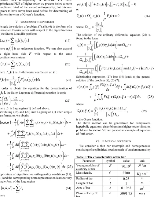
[image:3.595.55.560.85.727.2]

We consider a thin bar (isotropic and homogeneous), consisting of a cylindrical section made of an aluminum alloy Table I: The characteristics of the bar

Parameter symbol value unit

Young modulus of

elasticity of bar

E

9

70.10

N m

/

Mass density

ρ

₂₇₀₀

_/

3

Kg m

Radius of bar

r

0.25

m

Length of bar

l

1

m

Area of bar

_A

_0.1963

2

m

Phase velocity of bar

The elasticity constants of the surrounding medium at the both end of the bar are:

9 2 9 2

0

0.5 10 /

N m

and 10 /

l

N m

β

=

×

β

=

In what follows we use the mathematical software Mathcad to implement and numerically illustrate all the results. The Mathcad function “root” is used to solve the

transcendental equation

D

( )

ω

=

D

λ ω

( )

=

0

. To guess a starting value of each

ω

_n

,

n

=

1

,

2

,...

,

log ( )

D

ω

is plotted versus the frequency

f

=

ω π

( )

2

−1 (Fig 1) and some downward “spikes” are seen. Using the command “Trace” in Mathcad, the approximate value of ω at the

[image:4.595.311.541.55.237.2]

spikes is determined, that is

ω

=

2

π

f

.

[image:4.595.53.277.274.413.2]

Figure 1: Graph used to estimate the values of the eigenfrequencies

Table II: The first five eigenfrequencies of the bar

Eigenfrequency Symbol Value Unit

First mode

1

/ 2

ω

π

265.429

Hz

Second mode

2

/ 2

ω

π

_{2.574 10}

_×

3

_Hz

Third mode

3

/ 2

ω

π

_{5.106 10}

_×

3

_Hz

Fourth mode

4

/ 2

ω

π

_{7.647 10}

_×

3

_Hz

Fifth mode

5

/ 2

[image:4.595.243.545.336.749.2]

ω

π

_{1.019 10}

_×

4

_Hz

Table III: The first five natural frequencies Natural frequency Symbol Value Unit First mode

1

/ 2

π

Ω

265.429

Hz

Second mode

2

/ 2

π

Ω

_{2.574 10}

_×

3

_Hz

Third mode

3

/ 2

π

Ω

_{5.106 10}

_×

3

_Hz

Fourth mode

4

/ 2

π

Ω

_{7.647 10}

_×

3

_Hz

Fifth mode

5

/ 2

π

Ω

_{1.019 10}

_×

4

_Hz

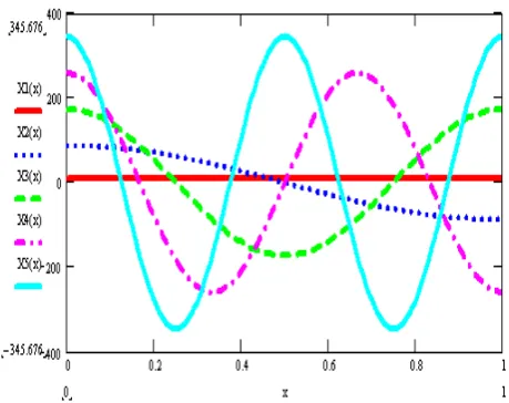
Figure 2: The eigenfunctions corresponding to the first five eigenvalues

Fig 2 shows different shapes of the vibration at different modes.

VII. GENERALISATION: RAYLEIGH-BISHOP EQUATION

In this section we give an example of application of our method to the vibration problem for a thick bar. This is more complicate problem leading to an equation of forth order. Rayleigh-Bishop theory for vibrating thick bar improve the classical theory by taking into account the lateral displacements (characterize by the Poisson ratio

η

) and the effects of shear stiffness accompanying this transverse displacement while calculating the strain energy by introducing the bulk modulus of second kind

μ

. [2], [3]. In this case the displacements are assumed as follow:

( )

(

)

(

,

,

)

.

,

,

,

,

,

u

z

t

z

x

w

w

u

y

t

y

x

v

v

t

x

u

u

′

−

=

=

′

−

=

=

=

η

η

The Lagrangian is given by:

(

)

(

′

+

′′

)

+

−

−

+

′

+

=

∫

∫

∫

dx

u

I

u

EA

Audx

t

x

F

dx

u

I

u

A

L

p p

1

0

2 2 2

1

0 1

0

2 2 2

2

1

)

,

(

2

1

μ

η

η

ρ

The equation of motion has the form [2]:

( )

,

,

(30)

)

,

(

)

,

(

)

,

(

)

,

(

4 4 2

2 2 4 2 2

2

2 2

t

x

AF

x

t

x

u

I

t

x

t

x

u

I

x

t

x

u

EA

t

t

x

u

A

p

p

=

∂

∂

+

+

∂

∂

∂

−

∂

∂

−

∂

∂

η

μ

ρη

ρ

with the following boundary conditions

⎪⎭

⎪

⎬

⎫

=

′′

=

′′′

−

′

+

′

= =

0

0

1 , 0

1 , 0 2 2

x x p p

u

u

I

u

EA

u

I

μ

η

ρη

(31)

[image:4.595.42.287.448.571.2]

The Sturm-Liouville problem is: Equation for eigenfunction

y

=

y

( )

x

is

(

)

4 2

2 2 2 2

4 2

(32)

p p

d y

d y

I

I

EA

Ay

dx

dx

μ η

+

λ ρη

−

=

λ ρ

Boundary conditions are

(

)

⎪⎭

⎪

⎬

⎫

=

′′

=

′′′

−

′

−

=

=

0

0

1 , 0

1 , 0 2 2

2

x

x p p

y

y

I

y

I

EA

λ

ρη

μ

η

(33)

The particular feature of Sturm- Liouville problem (32)-(33) is that eigenvalues

λ

arise in boundary conditions (33). The general theory of such problems is not developed at present. The latest results concerning this type of problems can be found in [7].

Orthogonalities [2]:

[

]

[

(

)

(

)

(

)

(

)

]

,

and

)

(

)

(

)

(

)

(

2 2 1

0

2

2 1 1

0

2

nm n m

n p m

n

nm n m

n p m

n

y

dx

x

y

x

y

I

x

y

x

y

EA

y

dx

x

y

x

y

I

x

y

x

Ay

δ

μ

η

δ

η

=

′′

′′

+

′

′

=

′

′

+

∫

∫

Where

[

]

[

(

)

(

)

]

.

and

)

(

)

(

1

0

2 2 2

2 2

1

0

2 2 2

2 1

dx

x

y

I

x

y

EA

y

dx

x

y

I

x

Ay

y

n p n

n

n p n

n

∫

∫

′′

+

′

=

′

+

=

μ

η

η

The solution of the problem is of the form:

∫ ∫

∫

∫

−

+

+

⎥

⎦

⎤

⎢

⎣

⎡

∂

∂

′

+

∂

∂

∂

′

+

+

⎥⎦

⎤

⎢⎣

⎡

₊

∂

∂

=

t p

d

d

t

x

G

F

A

t

x

G

h

t

t

x

G

g

I

d

t

x

G

h

t

t

x

G

g

A

t

x

u

0 1

0 2

1

0

2 2

2 2

1

0 2

2

,

)

,

,

(

)

,

(

)

,

,

(

)

(

)

,

,

(

)

(

)

,

,

(

)

(

)

,

,

(

)

(

)

,

(

τ

ξ

τ

ξ

τ

ξ

ρ

ξ

ξ

ξ

ξ

ξ

ξ

η

ξ

ξ

ξ

ξ

ξ

where

∑

∞

=

Ω

Ω

=

1 _{2, 1}2

, 2 2

sin

)

(

)

(

)

,

,

(

n _{n n}

n n

n

y

t

y

x

y

t

x

G

ξ

ξ

is the

Green’s function in which _2, 2 1

n n

n

y

y

ρ

Ω =

is the

eigenfrequency

The generalization of this method is also possible for the above hyperbolic equation with variable coefficients [1].

VIII. CONCLUSIONS

In this paper Hamilton's variational principle has been the main mathematical tool of derivation of the equations of motion with associated boundary conditions. It has been demonstrated that from the orthogonality of the eigenfunctions (two kinds) of the Sturm-Liouville problem, we can easily formulate the solution of the of vibration problem.

REFERENCES

[1] I. Fedotov, A.D. Polyanin and M. Shatalov. (2007, February). Theory of free vibration of rigid rod based on the Raleigh model. Doklady Physics. (417). pp. 56-61.

[2] I. Fedotov, Y. Gai, and M. Shatalov. (2006). Analysis of Rayleigh-Bishop Model. Electronic Transactions of Numerical analysis. (24). pp. 66-73.

[3] J.S. Rao, Advanced theory of vibration. New Delhi: Wiley Eastern Limited, 1992.

[4] J.W.S.Rayleigh, Theory of sound. New York: Dover, 1945.

[5] J.N. Reddy, Energy principles and variational methods in applied mechanics. 2nd _{ed. New Jersey: John Wiley & Sons, 2002.}

[6] S. Timoshenko et al., Vibration problems in Engineering. New York: John Wiley & Sons, 1974.