A Chart Re estimation Algorithm for a Probabilistic Recursive Transition Network

(1)

Probabilistic Recursive Transition

N e t w o r k

Y o u n g S. H a w University of Suwon

Key-Sun Choi*

Korea Advanced Institute of Science and Technology

A Probabilistic Recursive Transition Network is an elevated version of a Recursive Transition Network used to model and process context-free languages in stochastic parameters. We present a re-estimation algorithm for training probabilistic parameters, and show how efficiently it can be implemented using charts. The complexity of the Outside algorithm we present is O(N4G 3) where N is the input size and G is the number of states. This complexity can be significantly overcome when the redundant computations are avoided. Experiments on the Penn tree corpus show that re-estimation can be done more efficiently with charts.

1. Introduction

Though hidden Markov models have been successful in some applications such as corpus tagging, they are limited to the problems of regular languages. There have been attempts to associate probabilities with context-free grammar formalisms. Re- cently Briscoe and Carroll (1993) have reported work on generalized probabilistic LR parsing, and others have tried different formalisms such as LTAG (Schabes, Roth, and Osborne 1993) and Link grammar (Lafferty, Sleator, and Temperley 1992). Kupiec ex- tended a SCFG that worked on CNF to a general CFG (Kupiec 1991). The re-estimation algorithm presented in this paper may be seen as another version for general CFG.

One significant problem of most probabilistic approaches is the computational burden of estimating the parameters (Lari and Young 1990). In this paper, we consider a probabilistic recursive transition network (PRTN) as an underlying grammar rep- resentation, and present an algorithm for training the probabilistic parameters, then suggest an improved version that works with reduced redundant computations. The key point is to save intermediate results and avoid the same computation later on. Moreover, the computation of Outside probabilities can be made only on the valid parse space once a chart is prepared.

2. A Probabilistic Recursive Transition Network

A PRTN denoted by A is a 6-tuple.

= ( A , u , s , ; : , r , 5 ) .

* Computer Science Department, University of Suwon, Suwon P.O. Box 77-78, Suwon, 440-600, Korea. E-mail: [email protected]

(2)

Computational Linguistics Volume 22, Number 3

C F G N P ~ a r t A P n o u n

N P , A P n o u n

N P ~ n o u n

A P . a d j A P A P = a d j

PRTN

C a l l

i States n o u n 0.2

~.o o.8 ~

p a i

v ~ v o.~,,~

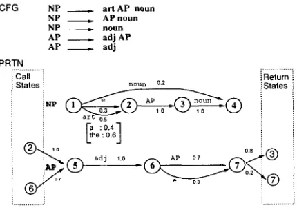
. . . J : ... Figure 1

Illustration of PRTN. A parse is composed of dark-headed transitions. i R e t u r n i States

~ @

A is a transition matrix containing transition probabilities, a n d B is a w o r d matrix containing the probability distribution of the words observable at each terminal transition. I? specifies the types of transitions, and ~ represents a stack. S a n d .~ denote start a n d final states, respectively.

Stack operations are associated w i t h transitions; transitions are classified into three types, according to the stack operation. The first type is nonterminal transition, in which state identification is p u s h e d into the stack. The second type is pop transition, in which transition is determined b y the content of the stack. The third type is transitions not committed to stack operation; these are terminal a n d e m p t y transitions. In general, the g r a m m a r expressed in PRTN consists of layers. A layer is a fragment of n e t w o r k that corresponds to a nonterminal. A table of the probability distribution of w o r d s is defined at each terminal transition. Pop transitions represent the returning of a layer to one of its (possibly multiple) higher layers.

In this paper, parses are a s s u m e d to be sequences of dark-headed transitions (see Figure 1). States at which pop transitions are defined are called pop states. Other notations are listed below.

first(1)

returns the first state of layer I.

last(l)

returns the last state of layer I.

layer(s)

returns the layer state s belongs to.

bout(1)

returns the states from which layer 1 branches out.

bin(1)

returns the states to which layer 1 returns.

terminal(1)

returns a set of terminal edges in layer 1.

nonterminal(1)

returns a set of nonterminal edges in layer I.

denotes the edge between states i a n d j.

[i,j] denotes the network segment b e t w e e n states i a n d j.

[image:2.468.136.351.50.202.2]

(3)

3. Re-estimation Algorithm

The task of a re-estimation algorithm is to assign probabilities to transitions and the word symbols defined at each terminal transition. The Inside-Outside algorithm pro- vides a formal basis for estimating parameters of context free languages so that the probabilities of the word sequences (sample sentences) may be maximized. The re- estimation algorithm for PRTN uses a variation of the Inside-Outside algorithm cus- tomized for PRTN.

Let a word sequence of length N be denoted by:

W = Wl Wa--.WN.

Now define the Inside probability.

Definition 1

The Inside probability denoted by

Pi(i)s~t

of state i is the probability that

layer(i)

generates the string positioned from s to t starting at state i given a model ,~.

That is:

Pi(i)s~t = P([i,e] --+ Ws~tl,~)

where e =

last(layer(i)).

And by definition:

t

P,(i)s~t = ~ aikb(T~, Ws)P,(k)s+l~t + ~ Y2 aijauvP,(j)s~rP,(v)r+l~t.

k j r=s

(1)

- - - + ___+

where

ik E terminal(layer(i)), ij E nonterminal(layer(i) ), u = last(layer(j)), v E bin(layer(j)),

and

layer(i) = layer(v).

After the last word is generated, the last state of

layer(i)

should be reached.

1 if i =

last(layer(i)),

Pl(i)t+l~t

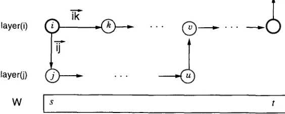
= 0 otherwise.

Figure 2 is the pictorial view of the Inside probability. A valid sequence can begin only at state $, thus to be strict, P1(8) has an additional product, P($). When

the immediate transition ~ is of terminal type, the transition probability

aq

and the

probability of the S th word at the transition b(~j,

Ws)

are multiplied together with the

Inside probability of the rest of the sequence,

Ws+l~t.

Now define the Outside probability.

Definition 2

The Outside probability denoted by

Po (i,j)s~t

is the probability that partial sequences,

Wl~s_l

and

Wt+l~N,

a r e generated, provided that the partial sequence,

Ws~t,

is gen-

erated by [i,j] given a model ~.

And by definition:

Po(i,j)s~t

= P([,S',i] --~ Wl~s_l, ~',..~-] - ~ -

Wt+l~ N

I A)

N

= ~ ~ ~ axfaeYPr(f'i)a~s-lPl(j)t+l~bPo(x,y)a~b •

x a = l

b=t

(4)

T~

layer(j)

, . , , = . . . .

W

I~

t I

Figure 2

Illustration of Inside probability.

,aye~Ix> _-

?

@

layer(i) ~

_{. . . . ~[)_~.... = ~ _ ~ . . . . _ ~}

w I'

s, I'

**'1'*'**

NI

Figure 3

Illustration of Outside probability.

where x E bout(layer(i)), y E bin(layer(i)), f =first(layer(i)), e = last(layer(i)), layer(i) = layer(]'), a n d layer(x) = layer(y).

The s u m m a t i o n on x is defined only w h e n a ~ 1 or b ~ N (i.e., there are words left to be generated). Nonterminal a n d its corresponding pop transitions are defined to be 1 w h e n a = 1 a n d b = N.

For a b o u n d a r y case of the Outside probability where f is the first state of a layer in the above equation:

1 i f f = $,

Po(i,j)l~S = 0 otherwise.

Figure 3 shows the n e t w o r k configuration in c o m p u t i n g the Outside probability. In equation 2, P~(f, i)~s-1 is the probability that sequence, W a ~ - l , is generated b y layer(i) left to state i, a n d

Pl(j)t+l~b

is the probability that sequence Wt+l~b is generated b y layer(i) right to state j.

The computation of P~ 0 c, i)s~t--a slight variation of the Inside probability in which the P~(f)a~b'S in equation 1 are replaced b y P~0 c, i)a~b--is done as follows:

P~(f,i)s~t

{ pl0C)s~t if s __q t,

= 1 if s > t a n d f = i, 0 if s > t a n d f ¢ i.

It is basically the same as the Inside probability except that it carries an i that indicates a stop state.

[image:4.468.102.384.56.169.2] [image:4.468.76.391.58.320.2]

(5)

function, w e h a v e the following form of re-estimation for each transition (Rabiner 1989).

expected n u m b e r of transitions from state i to state j expected n u m b e r of transitions from state i

The expectation of each transition type is c o m p u t e d as follows: For a terminal transition:

Y'~ffr=l aijb(~, W~)Po(i,j)~~~

Et( ij ) =

P(W I A)

For a n o n t e r m i n a l transition:

N

~s=l Y~fft-s aijP,(j)~ta~Po( i, v)s~t

Ent(~ ) =

_P(wl

w h e r e u =

last(layer(j)), v ¢ bin(layer(j)), layer(i) = layer(v), layer(j) = layer(u),

and uv is a p o p transition. For a p o p transition:

N N

~-~s=l

~-~t=s

&,vPl(v)s~taijPo(u, J)sNt

Go,( ij ) =

P(W I ,k)

w h e r e

u E bout(layer(i)), j c bin(layer(i)), v = first(layer(i)), layer(u) = layer(j), layer(v) =

layer(i),

a n d uv is a n o n t e r m i n a l transition.

Since transitions of terminal and n o n t e r m i n a l types can occur together at a state, terminal transitions are estimated as follows:

- - - +

a-ij

Gk Et(ik) + Gk Ent(~)

(3)

For n o n t e r m i n a l transitions:

E,,,( q)

(4)

A n d for p o p transitions, notice that only p o p transitions are possible at a p o p state:

L

aq

_ G o , ( q )

Y~k Epop( ik )

(5)

For a terminal transition ~ and a w o r d symbol w:

C t ~.,. w,=~,,

aijb(~, Wt)Po(i,j)t~t

b( ij,w)

=

Y'~fft=~ aqb(~, Wt)Po(i,j)t~t

(6)

sentence W

T Compute Inside probability 1

ofW [

Inside Table

Select valid Insides by [ ~ running Inside algorithm

topdown

of

valid Insides

Run Outside algorithm ]

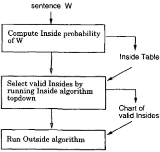
I Figure 4

Outside computation with chart. Inside computation builds a table of computed Insides.

4. Chart Re-estimation Algorithm

It can be shown that the complexity of the Inside algorithm is O(N3G 3) and that of the Outside algorithm is O(N4G 3) where N is the input size and G is the number of states. The complexity is too much for current workstations when either N or G becomes bigger than a few 10s. A basic implementation of the algorithm is to use a chart and avoid doing the same computations more than once. For instance, the table for storing Inside computations takes

O(N2G2C)

store, where C is the number of terminal and nonterminal categories. A chart item is a function of five parameters, and returns an Inside probability.

I(i,j, s, t, c) = Pi(i,j)s~t.

A chart item is associated with categories implying that the item is valid on the specified categories that begin the net fragment of the item. Suppose a net fragment [i,j] begins with NP and ADJP, then given a sentence fragment

Ws~t,

ADJP may not participate in generating

Ws~t,

while NP may. The information of valid categories is useful when the chart is used in computing Outside probabilities.

An Outside probability is the result of computing m a n y Inside probabilities. Com- puting an Inside probability even in an application of moderate size can be impractical. A naive implementation of Outside computation takes numerous Inside computations, so estimating even a parameter will not be realistic in a serial workstation (Lari and Young 1990).

The proposed estimation algorithm aims at reducing the redundant Inside computations in computing an Outside probability. The idea is to identify the Inside probabilities used in generating an input sentence and to compute an Outside probability using mainly those Insides. This is done first by computing an Inside probability of the input sentence, which can return a table of Insides used in the computation. Note that the Insides in the deepest depth are produced first, as the recursion is released, thus there can be m a n y Insides that are not relevant to the given sentence. The Insides that participate in generating the input sentence can be identified by running the In- side algorithm one more time, top-down. Figure 4 illustrates the steps of the revised Outside computation.

[image:6.468.170.331.49.202.2]

(7)

left to right and one transition at a time. Many Insides that are missed in the table are compositions of smaller Insides.

Once charts of selected Insides are prepared, an Outside probability is computed as follows:

Po(i,j)s~, = ~ ~ axfaevlOe, i,a,s - 1)I(j,e,t + 1, b)Po(x,y)a~b .

{xiI(x,y,a,b,c)>O} (a,b)ca(f,e,s,t)

where x E bout(layer(i)), y c bin(layer(i)), f = first(layer(i)), e = last(layer(i)), c c

{nonterminal}, layer(i) = layer(j), and layer(x) = layer(y).

The function cr0C, e,s, t) returns a set of (a, b) pairs where there are Inside items I0 c, e, a, b) defined at the chart such that a G s and b > t. In short, the items for state f indicate the possible combinations of sentence segments inclusive of the given fragment Ws~t because the chart contains items of all the valid sentence segments that were generated through the layer ~c, e]. When the current layer ~c, e] is completed with the two Insides computed, the computation extends to the Outside.

Useless advancements into high layers that do not lead to the successful comple- tion of a given sentence can be avoided by making sure that Ix, y] generates Wa~b and the category of current layer c is defined, which can be checked by consulting the chart items for state x.

5. Experiments

The goal of our experiments is to see how much saving the new estimation algorithm achieves in computational cost. Out of 14,132 Wall Street Journal trees of the Penn tree corpus, 1,543 trees corresponding to sentences with 10 words or less were chosen, and the programs written in C language were run at a Sparcl0 workstation.

The basic implementation of an Inside-Outside algorithm assumes tables for In- sides and Outsides so that identical Insides and Outsides need not be recomputed. A chart Outside or re-estimation algorithm assumes a refined table of Insides that contains only valid Insides used in generating the input sentence as discussed earlier, and Outside computation is done based on the refined table.

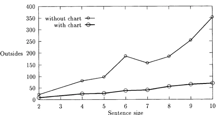
The improvement from the chart re-estimation algorithm is measured in the number of actual Inside and Outside computations done to estimate the parameters. Fig- ure 5 shows the average counts of Insides used in estimating 50 trees randomly selected from 1,543 samples. Before the re-estimation algorithm is applied, an RTN that faith- fully encodes the input trees without any overgeneration is constructed from the 50 trees. The gain in Insides from the chart re-estimation algorithm is very clear, and in the case of Outsides the gain is even more conspicuous (see Figure 6). The number of Insides counted in chart version also includes the Insides computed in preparing the chart.

6. Conclusion

(8)

Computational Linguistics Volume 22, N u m b e r 3

2000 I I I I

w i t h o u t c h a r t o + J

1500 wit r I ,

Insides 1000

5OO

0

0 2 4 6 8 10

S e n t e n c e size

Figure g

Gain in Insides using chart re-estimation, showing 50 r a n d o m l y - c h o s e n sentences out of 1,543 samples.

400 I I J I I I I |

,1,

350 w i t h o u t c h a r t o

w i t h ch 3O0

25O

O u t s i d e s 200

150

100

50

o _ . _ . _ _ . 7 - ~ o t .~ I I I I I

2 3 4 5 6 7 8 9 10

S e n t e n c e size

Figure 6

[image:8.468.88.417.93.279.2] [image:8.468.72.423.404.591.2]

(9)

References

griscoe, Ted, and John Carroll. 1993. Generalized probabilistic LR parsing of natural language (Corpora) with unification-based grammars." Computational Linguistics 19(1): 25-57. Kupiec, Julian. 1991. A trellis-based

algorithm for estimating the parameters of a hidden stochastic context-free grammar. In Proceedings of the Speech and Natural Language Workshop, pages 241-246, DARPA, Pacific Grove.

Lafferty, John, Daniel Sleator, and Davy Temperley. 1992. Grammatical trigrams: A probabilistic model of link grammar. AAAI Fall Symposium Series: Probabilistic

Approaches to Natural Language, pages 89-97, Cambridge.

Lari, K. and S. J. Young. 1990. The estimation of stochastic context-free grammars using the Inside-Outside algorithm. Computer Speech and Language 4:35-56.

Rabiner, Lawrence R. 1989. A tutorial on hidden Markov models and selected applications in speech recognition. In Proceedings of the IEEE 77, Volume 2. Schabes, Yves, Michael Roth, and Randy