The Photometric Maximum in Cosmicflows 2

(1)

http://www.scirp.org/journal/jhepgc ISSN Online: 2380-4335 ISSN Print: 2380-4327

DOI: 10.4236/jhepgc.2018.41011 Jan. 31, 2018 123 Journal of High Energy Physics, Gravitation and Cosmology

The Photometric Maximum in Cosmicflows-2

Lorenzo Zaninetti

Physics Department, via P. Giuria 1, Turin, Italy

Abstract

Based on well known photometric rules for the number of galaxies as function of the distance in Mpc we model the so called “Great Wall” which is visible on the Cosmicflows-2 catalog. The gravitational field is evaluated at the light of the shell theorem and a finite value for the gravitational field is numerically derived.

Keywords

Cosmology, Observational Cosmology, Distances, Redshifts, Radial Velocities, Spatial Distribution of Galaxies, Magnitudes and Colors, Luminosities

1. Introduction

Before to start we briefly review the Hubble law, after [1], which is a linear rela-tionship between expansion velocity and distance in

0 ,

V =H D=c z (1)

where H0 is the Hubble constant

1 1

0 100 km s Mpc

H = h ⋅ − ⋅ − , with h=1 when h is not specified, D is the distance in Mpc, c is the light velocity and z is the redshift. As an example a recent evaluation, see [2], quotes

(

)

1 1

0 74.4 3 km s Mpc .

H = ± ⋅ − ⋅ − (2)

The original Hubble’s law was based on ≈20 galaxies of which was known the distance and the velocity; conversely in the last years the number of catalogs for galaxies with redshift available for public downloading has progressively grown. This huge amount of data allows setting up critical tests between different theo-retical models over the various aspects of the Large Scale Structures. The layout of the paper is as follows. In Section 2, we describe some representative catalogs of galaxies. In Section 3, we introduce the adopted luminosity function for ga-laxies. In Section 4, we model the maximum in the number of galaxies as

func-How to cite this paper: Zaninetti, L. (2018) The Photometric Maximum in

Cosmic-flows-2. Journal of High Energy Physics,

Gravitation and Cosmology, 4, 123-131. https://doi.org/10.4236/jhepgc.2018.41011

Received: November 28, 2017 Accepted: January 28, 2018 Published: January 31, 2018

http://creativecommons.org/licenses/by/4.0/

(2)

DOI: 10.4236/jhepgc.2018.41011 124 Journal of High Energy Physics, Gravitation and Cosmology tion of the distance. In Section 5, we evaluate the gravitational field as produced by the visible galaxies of Cosmicflows-2 catalog. We conclude in Section 6.

2. The Catalogs of Galaxies

A first kind of catalog for galaxies is represented by those focused as slice as the two-degree Field Galaxy Redshift Survey, in the following 2dFGRS, see [3], or the Sloan Digital Sky Survey (SDSS), see [4]. A second classification is about the all-sky catalogs such as the 2MASS Redshift Survey (2MRS), see [5], or the Cos-micflows-2, see [2]. As a first example a strip of the 2dFGRS is shown in Figure 1. The below Figure, which is a 3˚ slice, shows that the galaxies resides on fila-ments rather to be distributed in a uniform 2D way. A first extrapolation allows to state that the galaxies are disposed on the surface of bubbles rather than to fill uniformly the 3D space. The statistics of the voids is a topic of research and an important parameter is the average radius of the voids, R : [6] quotes

1

18.23 Mpc

R = h− and Table 1 in [7] quotes a variable average radius ranging

from 1

15.964 Mpc

R = h− to R =63.347h−1Mpc according to the selected

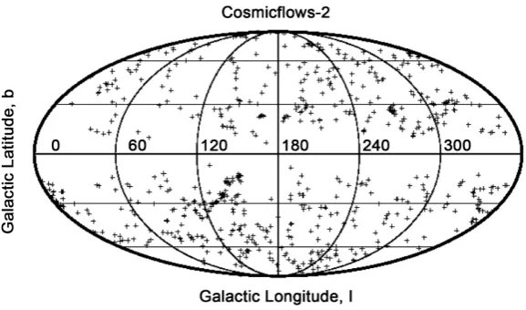
sample. As second example is represented by the overall Cosmicflows-2 catalog, data available at http://vizier.u-strasbg.fr/viz-bin/VizieR, and Figure 2 reports the sky distribution of such a catalog in Galactic coordinates.

Also in this case the voids are can be visualized selecting a thin (20 Mpc) spherical shell, see Figure 3.

3. Luminosity Function for Galaxies

The distance modulus is

( )

5log 5,

[image:2.595.276.474.443.680.2]

m−M = d − (3)

(3)

[image:3.595.229.519.71.237.2]

DOI: 10.4236/jhepgc.2018.41011 125 Journal of High Energy Physics, Gravitation and Cosmology Figure 2. Sky distribution of 4970 Cosmicflows-2’s galaxies in galactic coordi-nates projected using the Mollweide projection.

Figure 3. Sky distribution of 713 Cosmicflows-2’s galaxies with distance ∈

[63.8 Mpc, 83.8 Mpc].

where m is the apparent magnitude, M is the absolute magnitude and d is the distance in pc.

Let L, the luminosity of a galaxy, be defined in

[ ]

0,∞ . The Schechter LF of galaxies, Φ_{, see [8], is}

(

)

*

* *

* * *

; , , d L exp L d ,

L L L L

L L L

α

α Φ    

Φ Φ =_ _{ } _− _

   

  (4)

where

α

sets the slope for low values of L, L* is the characteristic luminos-ity, and _Φ*_{represents the number of galaxies per Mpc}3_{. The normalization is}

(

* *

)

*

(

)

0 L; , ,α L dL α 1 ,

∞

Φ Φ = Φ Γ +

∫

(5)

where

( )

1

0

Γ z =

∫

∞ − −et zt d ,t (6)

[image:3.595.230.519.280.450.2]

(4)

DOI: 10.4236/jhepgc.2018.41011 126 Journal of High Energy Physics, Gravitation and Cosmology

(

* *

)

* *

(

)

; , , 2 .

L

α

L L

α

Φ Φ = Φ Γ + ₍₇₎

An equivalent form in absolute magnitude of the Schechter LF is

(

)

_0.4( ₁)

(

*

)

_0.4

(

*

)

* * *

; , , d 0.921 10 M M exp 10 M M d ,

M

α

M M α+ −  −  M

Φ Φ = Φ _− _

  (8)

where *

M is the characteristic magnitude.

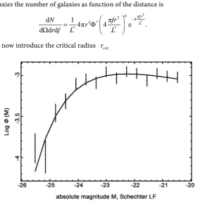
[image:4.595.206.540.181.682.2] [image:4.595.231.520.392.678.2]

A typical result of the Schechter LF in the case of Cosmicflows-2 is reported in Figure 4.

4. The Photometric Maximum

The flux, f, is

2,

4π

L f

r

= (9)

where r is the distance and L the luminosity of the galaxy. The joint distribution in distance, r, and flux, f, for the number of galaxies is

2

* 2

0

d 1

4π d ,

d d d 4π 4π

N L L

r r f

r f L δ r

∞    

= Φ_ _ _ − _

Ω

∫

    (10)

were the factor ( 1

4π) converts the number density into density for solid angle

and the Dirac delta function selects the required flux. In the case of Schechter LF of galaxies the number of galaxies as function of the distance is

2 * π 2 ₄ 4 * * *

d 1 π

4π 4 e .

d d d

fr L

N fr

r

r f L L

α −

 

= Φ  

Ω _ _ (11)

We now introduce the critical radius rcrit

Figure 4. The observed Schechter LF for galaxies of Cosmicflows-2, empty stars with error bar, and the fit by the Schechter LF when

* 3 3

0.0018 Mpc

(5)

DOI: 10.4236/jhepgc.2018.41011 127 Journal of High Energy Physics, Gravitation and Cosmology * 1 . 2 π crit L r f

= (12)

Therefore the joint distribution in distance and flux becomes 2 2 2 4 * * 2 d 1

4π e .

d d d

crit r r crit N r r

r f L r

α ₋

 

= _{Φ } _

Ω _ _ (13)

The above number of galaxies has a maximum at r=rmax:

max 2 crit,

r = +αr (14)

and the average distance of the galaxies, r , is

(

3

)

. 5 2 crit r r α α Γ + =  

Γ_ + _

 

(15)

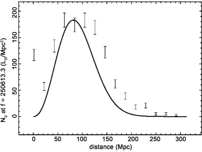
[image:5.595.205.539.68.272.2] [image:5.595.211.534.383.626.2]

Figure 5 presents the number of galaxies observed in Cosmicflows-2 as a function of the distance for a given window in flux, as well as the theoretical curve. The luminosity of a galaxy is produced and attenuated according to the electromagnetism. We now deal with the mass of a galaxy. A transformation of the luminosity of a galaxy, L, by the mass, , is given by the nonlinear For-mula (9) in [9]

Figure 5. The galaxies of Cosmicflows-2 with 2 2

12498.8L_ Mpc ≤ ≤f 488727.8L_ Mpc are organized by frequency versus distance, (empty circles); the error bar is given by the square root of the frequency. The maximum frequency of the observed galaxies is at

73.8

d= Mpc. The full line is the theoretical curve generated by d

d d d

N r f

Ω as given by

the application of the Schechter LF which is Equation (11) and the theoretical maximum is at d=81.69 Mpc. The parameters are * 10

1.8 10

(6)

0.32

10

2.35 .

10

L

L L

 

= _ _  

 ₍₁₆₎

We pay careful attention to the interval of existence in absolute magnitude ver-sus distance for Cosmicflows-2 catalog, see Figure 6.

The progressive decrease of the interval of existence for the absolute magni-tude is known as Malmquist bias [10]. Conversely the mass of a galaxy does not disappear with distance and therefore produce the gravitational field even if the galaxy is not visible due to the instrumental limitations.

5. Gravitational Forces

The shell theorem, according to proposition LXX, theorem XXX, in Principia [11] states that “If to every point of a spherical surface there tend equal centri-petal forces decreasing in the square of the distances from those points, I say, that a corpuscle placed within that superficies will not be attracted by those forces any way” or more simply “The gravitational field inside a uniform spher-ical shell is zero” [12] [13] [14]. The galaxies are thought to reside on irregular shells which are approximated by a given radius. Due to the fact that the shapes of the above shells are neither exactly spherical nor uniformly populated by ga-laxies we search for a low value of the gravitational field rather than the theoret-ical zero. We therefore analyze a 2D box with size of 30 Mpc and masses as given by formula 16. The forces in every point of the considered box are evaluated ac-cording to the Newtonian force where G, the Newtonian constant of gravitation, is

6 3 2

4.49975 10 Mpc gal yr8 ,

[image:6.595.230.523.435.666.2]

G= × − M ⋅ (17)

Figure 6. The absolute magnitude M of 4970 galaxies belonging to Cosmic-flows-2 when the absolute bolometric magnitude is 3.39 and

1 1

0 74.4 km s Mpc

H = ⋅ − ⋅ − (green points). The upper theoretical curve,

(7)

DOI: 10.4236/jhepgc.2018.41011 129 Journal of High Energy Physics, Gravitation and Cosmology where the length is in Mpc, mass is in Mgal which are

11

10 M_ and yr 8 are 108_{yr, see more details in [15]. The masses do not disappear with distance and}

[image:7.595.229.519.172.380.2]

the above value of the box allows processing a complete sample of galaxies. Fig-ure 7 reports the values of the gravitational field as a cut in the middle of the 2D box.Figure 8 reports the values of the gravitational field organized as a two col-or map.

Figure 7. Cut-line of the 2D gravitational forces expressed in 2

Mpc⋅M_gal yr8 (decimal logarithm).

Figure 8. Color scheme for the values of the gravitational field evaluated in 500 × 500 points. The red zone has values of gravitational field in the interval

2 2

4.27 Mpc M_gal yr8 , 0.00017 Mpc M_gal yr8

 ⋅ ⋅ 

  (the zones near the galaxies)

and the green zone has values of gravitational field in the interval

2 8 2

0.00017 Mpc M_gal yr8 ,1.7 10 Mpc− M_gal yr8

 ⋅ × ⋅ 

[image:7.595.259.486.430.647.2]

(8)

6. Conclusion

The observed “great wall” is theoretically explained by a maximum in the num-ber of galaxies as function of the distance in Mpc, see Figure 5. The two con-cepts of repeller and attractor, see [16], are not used in our analysis. The pres-ence of voids approximated by spheres in the spatial distribution of galaxies al-lows analyzing the gravitational field at the light of the shell theorem. Due to the facts that the number of galaxies is finite and the masses of galaxies are distri-buted according to a gamma probability density function the gravitational field

at the center of the voids turns out to be 8 2

2 10 Mpc Mgal yr8

−

≈ × ⋅ rather than

zero.

Acknowledgements

This research has made use of the VizieR catalogue access tool, CDS, Strasbourg, France.

References

[1] Hubble, E. (1929) A Relation between Distance and Radial Velocity among Ex-tra-Galactic Nebulae. Proceedings of the National Academy of Science, 15, 168-173.

https://doi.org/10.1073/pnas.15.3.168

[2] Tully, R.B., Courtois, H.M., Dolphin, A.E., et al. (2013) Cosmicflows-2: The Data. Astronomical Journal, 146, 86. https://doi.org/10.1088/0004-6256/146/4/86

[3] Colless, M., Dalton, G., Maddox, S., et al. (2001) The 2dF Galaxy Redshift Survey: Spectra and Redshifts. Monthly Notices of the Royal Astronomical Society, 328, 1039-1063. https://doi.org/10.1046/j.1365-8711.2001.04902.x

[4] Berlind, A.A., Frieman, J., Weinberg, D.H., et al. (2006) Percolation Galaxy Groups and Clusters in the SDSS Redshift Survey: Identification, Catalogs, and the Multip-licity Function. Astrophysical Journal Supplement Series, 167, 1-25.

https://doi.org/10.1086/508170

[5] Huchra, J.P., Macri, L.M., Masters, K.L., et al. (2012) The 2MASS Redshift Sur-vey—Description and Data Release. Astrophysical Journal Supplement Series, 199,

26. https://doi.org/10.1088/0067-0049/199/2/26

[6] Pan, D.C., Vogeley, M.S., Hoyle, F., Choi, Y.Y. and Park, C. (2012) Cosmic Voids in Sloan Digital Sky Survey Data Release 7. Monthly Notices of the Royal Astronomi-cal Society, 421, 926-934. https://doi.org/10.1111/j.1365-2966.2011.20197.x

[7] Mao, Q., Berlind, A.A., Scherrer, R.J., et al. (2017) A Cosmic Void Catalog of SDSS DR12 BOSS Galaxies. Astrophysical Journal, 835, 161.

https://doi.org/10.3847/1538-4357/835/2/161

[8] Schechter, P. (1976) An Analytic Expression for the Luminosity Function for Ga-laxies. Astrophysical Journal, 203, 297-306. https://doi.org/10.1086/154079

[9] Cappellari, M., Bacon, R., Bureau, M., Damen, M.C., et al. (2006) The SAURON project-IV. The Mass-to-Light Ratio, the Virial Mass Estimator and the Fundamen-tal Plane of Elliptical and Lenticular Galaxies. Monthly Notices of the Royal Astro-nomical Society,366, 1126-1150. https://doi.org/10.1111/j.1365-2966.2005.09981.x

[10] Malmquist, K.G. (1920) A Study of the Stars of Spectral Type A. Meddelanden fran Lunds Astronomiska Observatorium Series II, 22, 1.

(9)

DOI: 10.4236/jhepgc.2018.41011 131 Journal of High Energy Physics, Gravitation and Cosmology Regiae ac Typis Josephi Streater, London.

[12] Arens, R. (1990) Newton’s Observations about the Field of a Uniform Thin Spheri-cal Shell. Note di Matematica, 10, 39.

[13] Chandrasekhar, S. (1995) Newton’ Principia for the Common Reader. Clarendon, Oxford.

[14] Borghi, R. (2014) On Newton’s Shell Theorem. European Journal of Physics, 35, Article ID: 028003.https://doi.org/10.1088/0143-0807/35/2/028003

[15] Zaninetti, L. (2012) The Intergalactic Newtonian Gravitational Field and the Shell Theorem. Serbian Astronomical Journal, 185, 17-23.