Generalised Test For C- Matched Samples
Umeh, Edith. U, OyekaI. C.A, Onyiorah, I.V., Onyiorah, A. A., Efobi,C.C
Abstract: This paper proposes a generalized statistical method for the analysis of multiple responses or outcome data in case control studies including situations in which the observations are either continuous or frequency data. Test statistics are proposed for assessing the statistical significance of differences between case-control response scores. The proposed methods are illustrated with some sample data. When there are only three possible response options in which the proposed method and the Stuart/Maxwell test can be equally used to analyze the data; the proposed test statistic is shown to be at least as powerful as the Stuart/Maxwell test statistic.
Keywords: Generalised Test, Multiple Responses, Standard and Control Drug, Staurt/ Maxwell Test, Test Statistic
————————————————————
1.
Introduction
Often in controlled comparative prospective or retrospective studies involving matched samples of subjects or patients, the response of a subject to a predisposing factor in a retrospective study or to a condition or treatment in a prospective study, may be much finer than simply dichotomous. For example in a retrospective study where the predisposing factor maybe a subject’s employment status, a subject maybe classified as unemployed, self employed, public servant, student, housewife etc. In a prospective study involving some conditions or tests, subjects or patients maybe classified as recovered, much improved, improved, no change, worse or dead. A treatment or drug may be graded as very effective, effective, ineffective etc. If there are only three possible response options or categories, then the Stuart-Maxwell test (Fleiss 1974, Robertson et al 1994, Schlesselman 1982, Zhao and Kolonel 1992, Box and Cox 1964, Maxwell 1970, Stuart 1955, Fleiss 1981, Everitt 1977) may be used to analyse the data. We however here present a more generalized approach to the problem.
2.
The Proposed Method
In general, suppose we have a random sample of n - pairs of patients or subjects matched on a number of characteristics to be exposed to two experimental conditions, treatments, drugs or tests. Suppose further that the responses of these pairs of subjects are more than dichotomous but numbering c (c≥2) possible response options. Suppose further that 𝑖𝑡 pair of patients is selected, for i = 1, 2, … ,n and one member of the pair is randomly assigned to one of the treatments 𝑇1 ( standard drug; control), say, and the remaining member of the pair is assigned to the second treatment 𝑇2 (new drug; case) say, and the various c (c≥2) possible responses are recorded for each subject. That is the responses of each matched pair of subjects are classified into c mutually exclusive categories or classes. The appropriate data presentation format is as in
___________________________
UMEH, E. U, Department of Statistics, Nnamdi
Azikiwe University,P.O.Box 5025, Awka, Anambra State, Nigeria, Tel: +234- 8035503383
Email: [email protected],
I.C.A, OYEKA, Department of Statistics, Nnamdi
Azikiwe University, P.O.Box 5025, Awka,
Anambra State, Nigeria
I.V., ONYIORAH, Department of Pathology,
Nnamdi Azikiwe University Teaching Hospital, Nnewi
A.A., ONYIORAH, Department of Ophthalmology,
Enugu State University Teaching Hospital, Parklane Enugu
C.C., EFOBI, Department of
Table 1
Table 1: Format for Presentation of Data on ‘c’ Outcomes in Matched Pairs
Outcome Category for Control (Standard 𝑇1)
Outcome Category for Cases
(Experimental Condition 𝑇2) 1 2 . . . c Total(𝑛𝑖.)
1 𝑛11 𝑛12 . . .𝑛1𝑐 𝑛1.
2 𝑛21 𝑛22 . . .𝑛2𝑐 𝑛2.
. . . . .
. . . . .
. . . . .
C 𝑛𝐶1 𝑛𝐶2 . . . 𝑛𝐶𝐶 𝑛𝐶.
Total 𝑛.𝑗 𝑛.1 𝑛.2 . . . 𝑛.𝑐 n = 𝑛... (Miettinen 1969, Box and Cox 1964))
Each entry in Table 1 consists of a matched pair of case and control subjects. For example 𝑛11 is the numbers of
matched pairs of subjects in which both the case and control subjects are in category 1 response; 𝑛12 is the number of pairs in which the case is in category 1 response and the control subject is in category 2 response or in outcome category 2; and in general 𝑛1𝑗 is the number of
pairs in which the case is in category ‘I’ response while the corresponding control subject is in outcome or response category ‘j’. Also 𝑛1. is the total number of pairs in which
the case is in category 1 response, 𝑛.2 is the total number of
pairs in which the control subject is category 2 response. In general 𝑛𝑖. 𝑎𝑛𝑑 𝑛.𝑗 are respectively the total number of pairs
in which the case is category ‘I’ response and the control is in category ‘j’ response for 𝑖 = 1, 2, … , 𝑐, 𝑗 = 1, 2, … , 𝑐.
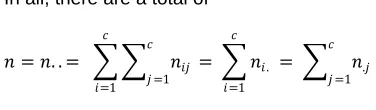
In all, there are a total of
𝑛 = 𝑛. . = 𝑛𝑖𝑗 𝑐
𝑗 =1 𝑐
𝑖=1
= 𝑛𝑖. 𝑐
𝑖=1
= 𝑛.𝑗 𝑐
𝑗 =1
subjects studied.
As in the Stuart/ Maxwell methods, let the difference between the number of pairs of respondents in the 𝑖𝑡
category of responses for case and 𝑖𝑡 category of responses for control be
𝑑𝑖 = 𝑛𝑖.− 𝑛.𝑖
(Miettinen, 1969, Maxwell 1970,
Everitt, 1977, Stuart, 1955) ……. 1
which is independent of 𝑛𝑖𝑖, 𝑖 = 1, , … , 𝑐, 𝑡𝑒 number of pairs in which both case and control subjects have the same response or outcome. Also let
𝑑𝑖𝑗 = 𝑛𝑖𝑗− 𝑛𝑗𝑖 ……… 2
which is the difference between the number of pairs in which the case is in the response category 𝑖 and the control is in the response category j and the number of pairs in
which the case is in response category j and the control is in the response category 𝑖; 𝑖 = 1, 2, … , 𝑐; 𝑗 = 1, 2, … , 𝑐; 𝑖 ≠ 𝑗.
Now having selected our random sample of n matched pairs, let 𝑥𝑖1 be the response by a member of the randomly
selected 𝑖𝑡 pair of patients or subjects randomly assigned treatment 𝑇1 (control standard drug) and 𝑥𝑖2 be the
response by the other member of the pair of patients or
subjects assigned treatment 𝑇2 𝑐𝑎𝑠𝑒, 𝑛𝑒𝑤 𝑑𝑟𝑢𝑔 for
𝑖 = 1, 2, … , 𝑛. We here assume for ease of presentation but without loss of generality, that the c mutually exclusive possible response categories have been ordered from the highest or most serious (lowest or least serious) level of response to the lowest or least serious (highest or most serious) level of response . for example, a patient’s response to a treatment for an illness or disease may range from recovered , most improved, through no change to worse or death; a subject response to a screening test may range variously from definitely positive to definitely negative. For candidate’s or student’s performance in a job interview or examination may range from very poor to excellent etc.
𝑜𝑟 𝑠𝑢𝑏𝑗𝑒𝑐𝑡𝑠 𝑎𝑠𝑠𝑖𝑔𝑛𝑒𝑑 𝑡𝑟𝑒𝑎𝑡𝑚𝑛𝑡𝑇2 𝑐𝑎𝑠𝑒 is a higher or more
𝑢𝑖 = 1, 𝑖𝑓 𝑥𝑖2, 𝑡𝑒 𝑟𝑒𝑠𝑝𝑜𝑛𝑠𝑒 𝑏𝑦 𝑡𝑒 𝑚𝑒𝑚𝑏𝑒𝑟 𝑖𝑛 𝑡𝑒 𝑖𝑡 𝑝𝑎𝑖𝑟 𝑜𝑓 𝑝𝑎𝑡𝑖𝑒𝑛𝑡𝑠 or subjects assigned treatment 𝑇2 (case) is a higher or
more serious () level of response than, the response by the other member of the pair assigned treatment 𝑇1 (control) for
all the c response categories.
0, if 𝑥𝑖1 and 𝑥𝑖2 are the same level of response for the two patients or subjects in the 𝑖𝑡 pair for all the c response
categories
-1, if 𝑥𝑖2 the response by the member in the 𝑖𝑡 pair of patients or subjects assigned treatment 𝑇2 (case) is a lower or
less serious (higher or more serious) level of response than 𝑥𝑖1 the response by the other member of the pair assigned
treatment 𝑇1 (control) for all the c response categories …………3
For 𝑖 = 1, 2, … , 𝑛
This means that 𝑢𝑖 assumes the value 1, if the response of the member of the 𝑖𝑡 pair of patients administered treatment 𝑇2 (case) is a higher or more serious (lower or
less serious) level of response than the response of the other member of the pair administered treatment 𝑇1
(control); 0, if the response of the two members of the pair are the same; and -1 , if the response of the member of the
𝑖𝑡 pair of patients administered treatment 𝑇
2 (case) is a
lower or less serious(higher or more serious) level of response than the response of the other member of the pair administered treatment 𝑇1 (control) for all the c response categories.
Now let
π+= 𝑃 𝑢
𝑖= 1 ; π0= 𝑃 𝑢𝑖= 0 ; π−= 𝑃 𝑢𝑖= −1 ..…..4
Where
π++ π0+ π−= 1 ……5
Let
𝑊 = 𝑛𝑖=1𝑢𝑖 …….6
Now
𝐸 𝑢𝑖 = π+− π− ……..7
And
𝑉𝑎𝑟 𝑢𝑖 = π++ π−− 𝜋+− 𝜋− 2 ..…..8
Also
𝐸 𝑊 = 𝑛𝑖=1𝐸𝑢𝑖= 𝑛 𝜋+− 𝜋− ……9
Note that 𝜋+− 𝜋− is the differential response rate between
the sub-populations administered treatments 𝑇2 (case) and 𝑇1(control) respectively in the paired population of patients or subjects for all the c response categories and is estimated by
𝜋+− 𝜋−= 𝑊
𝑛 ……. 10
Note also that 𝜋+, 𝜋0 and 𝜋− which are respectively the
probabilities that a randomly selected case is at a higher (or more serious) level, the same or lower (or less serious)
level of response than the corresponding control subject in the pair for all the c response categories are estimated using the notations in Table 1 and following the specifications in Equation 3 as
𝜋 += 𝑝+= 𝑓+ 𝑛 =
𝑛𝑖𝑗 𝑐 𝑗 =2 𝑐−1 𝑖=1
𝑖<𝑗
𝑛 …..11
𝜋 0 = 𝑝0= 𝑓0 𝑛 =
𝑛𝑖𝑖 𝑐 𝑖=1
𝑛 ….12
And
𝜋 −= 𝑝−= 𝑓− 𝑛 =
𝑛𝑖𝑗 𝑐−1 𝑗 =1 𝑐 𝑖=2
𝑖>𝑗
𝑛 …… 13
Where 𝑓+, 𝑓0 𝑎𝑛𝑑 𝑓− are respectively the number of 1s, 0s
and -1s in the frequency distribution of the n values of these numbers in 𝑢𝑖 in accordance with Equation 3
Hence using these results in 10 we have
𝑤 = 𝑓+− 𝑓−= 𝑛 𝑖𝑗 𝑐
𝑗 =2 𝑐−1
𝑖=1
− 𝑛𝑖𝑗 𝑐−1
𝑗 =1 𝑐
𝑖=2 𝑖 < 𝑗𝑖 > 𝑗….. 14
Furthermore the variance of W is obtained as
𝑉𝑎𝑟 𝑤 = 𝑉𝑎𝑟(𝑢𝑖 𝑛
𝑖=1
) + 𝑛
2 𝑐𝑜𝑣 𝑢𝑖, 𝑢𝑗
= 𝑛𝑉𝑎𝑟 𝑢𝑖 + 𝑛2 𝑐𝑜𝑣 𝑢𝑖, 𝑢𝑗 𝑖 < 𝑗𝑖 < 𝑗
Where Var( 𝑢𝑖 is given by Equation 8 and
𝑐𝑜𝑣 𝑢𝑖, 𝑢𝑗 = 𝐸𝑢𝑖𝑢𝑗 − 𝐸𝑢𝑖𝑢𝑗
Now 𝑢𝑖𝑢𝑗 can assume only the values 1,0, −1
𝑢𝑖𝑢𝑗 = 1, if 𝑢𝑖 𝑎𝑛𝑑 𝑢𝑗 are both equal to 1 or both equal to -1 with probabilities 𝜋+ 2+ 𝜋− 2, the value 0, if 𝑢
𝑖 and 𝑢𝑗
both assume the value 0, or 𝑢𝑖 assume the value 0 no matter the values assumed by 𝑢𝑗, or 𝑢𝑗 assumes the value
2𝜋0 𝜋++ 𝜋− + 𝜋0 2; and the value −1 if 𝑢
𝑖 assumes the
value 1 and 𝑢𝑗 assumes the value −1, or 𝑢𝑗 assumes the value 1 and 𝑢𝑖 assumes the value −1 with probability
𝜋+𝜋−+ 𝜋−𝜋+= 2𝜋+𝜋−
Hence
𝐸𝑢𝑖𝑢𝑗 = 1 𝜋+ 2+ 𝜋− 2+ 0 2𝜋0 𝜋++ 𝜋− + 𝜋0 2+ −1 = 𝜋+ 2+ 𝜋− 2− 2𝜋+𝜋−= 𝜋+− 𝜋− 2
So that using Equation 7, we have that
𝐶𝑜𝑣 𝑢𝑖𝑢𝑗 = 𝜋+− 𝜋− 2− 𝜋+− 𝜋− 2 = 0
Hence from Equation 8, we have that
𝑉𝑎𝑟 𝑤 = 𝑛 𝜋++ 𝜋−− 𝜋+− 𝜋− 2
……….. 15
Or equivalently using Equation 10, we have that
𝑉𝑎𝑟 𝑤 = 𝑛 𝜋++ 𝜋− −𝑊2 𝑛
……… 16
As noted above 𝜋+ is the proportion of pairs of case and
control subjects in which on the average the response rate by the sub-population of patients or subjects administered treatment 𝑇2 (new drug, case) is greater (less) than the
response rate by the sub-population of patients or subjects administered treatment 𝑇1 (standard drug, control); while 𝜋−
is the proportion of pairs in which on the average response rate by the sub- population of patients or subjects administered treatment 𝑇1 (standard drug, control) is greater (less than the response rate by the sub-population of patients administered treatment 𝑇2 (new drug, case) in
the paired population of patients for all response categories. Hence the null hypothesis that there exists no difference between the response rates by the sub-population of patients administered treatment 𝑇2 (new drug, case) and the sub-population of patients administered treatment 𝑇1
(standard drug, control) in the paired population of patients for all response categories is equivalent to the null hypothesis
𝐻0: 𝜋+− 𝜋−= 0 𝑣𝑒𝑟𝑠𝑢𝑠 𝐻
1: 𝜋+− 𝜋−≠ 0
……… 17
To test this null hypothesis, we may use the test statistic
𝜒2= 𝑊2 𝑉𝑎𝑟 𝑊 =
𝑊2
𝑛 𝜋+−𝜋− −𝑊 2 2
……….. 18
which under 𝐻0 has approximately a chi- square distribution
with 1 degree of freedom for sufficiently large n. Although strictly speaking the test statistic in Equation 18 has a
Chi-square distribution with 1 degree of freedom; however because its construction in equation 3 involves a combination of some c response categories, to help increase its power and reduce the chances of erroneously accepting a take null hypothesis (Type 1 error), it is here recommended that all comparisons should be made against critical Chi- Square values with c-1 degrees of freedom. Hence here 𝐻0 is rejected at the 𝛼 level of significance if
𝜒2≥ 𝜒
1−𝛼, 𝑐−12 , otherwise 𝐻0 is accepted.
In practical applications and use 𝜋+𝑎𝑛𝑑 𝜋− in Equation 18
are replaced by their sample estimates given in Equations 11 and 13 respectively so that
𝑛 𝜋 +− 𝜋 − = 𝑛 𝑖𝑗 𝑐 𝑗 =2 𝑐−1
𝑖=1 + 𝑐𝑖=2 𝑐−1𝑗 =1𝑛𝑖𝑗
………. 19
Hence the test statistic (Equation 18) becomes
𝜒2=
𝑛𝑖𝑗 𝑐 𝑗 =2 𝑐−1 𝑖=1 𝑖<𝑗 − 𝑛𝑖𝑗 𝑐−1 𝑗 =1 𝑐 𝑖=2 𝑖>𝑗 2 𝑛𝑖𝑗 𝑐 𝑗 =2 𝑐−1 𝑖=1 𝑖<𝑗 + 𝑛𝑖𝑗 𝑐−1 𝑗 =2 𝑐 𝑖=1
𝑖>𝑗 −
𝑛 𝑖𝑗 𝑐 𝑗 =2 𝑐−1 𝑖=1 𝑖<𝑗 − 𝑛 𝑖𝑗 𝑐−1 𝑗 =2 𝑐 𝑖=1 𝑖>𝑗 𝑛 2 ………..20
Note that if 𝑐 = 2, equation 20 under 𝐻0 reduces to a
modified version of the McNemar test statistic which is
𝜒2= 𝑛12−𝑛212 𝑛12+𝑛21− 𝑛 12−𝑛 21 2𝑛
……….. 21
which has a chi- square distribution with 𝑐 − 1 = 2 − 1 = 1
degree of freedom. Note that equation 21 has smaller variance than the usual McNemar test because of its modification to provide for possible ties between case and control subject pairs in their responses.
If 𝑐 = 3, equation 20 under 𝐻0 reduces to
𝜒2= 𝑛12−𝑛21 + 𝑛13−𝑛31 + 𝑛23−𝑛32 2
𝑛12+𝑛13+𝑛21+𝑛23+𝑛31+ 𝑛32 − 𝑛 12−𝑛 21 + 𝑛 13−𝑛 31 + 𝑛 23−𝑛 32 2
𝑛
………..22
which has a chi-square distribution with 𝑐 − 1 = 3 − 1 = 2
degrees of freedom. If 𝑐 = 4, equation 20 becomes
𝜒2
= 𝑛12− 𝑛21 + 𝑛13− 𝑛31 + 𝑛14− 𝑛41 + 𝑛23− 𝑛32 + 𝑛24− 𝑛42 + 𝑛34− 𝑛43 2
𝑛12+ 𝑛13+ 𝑛14+ 𝑛23+ 𝑛24+ 𝑛34+ 𝑛21+ 𝑛31+ 𝑛41+ 𝑛32+ 𝑛42+ 𝑛43−
𝑛12−𝑛21 + 𝑛13−𝑛31 + 𝑛14−𝑛41 + 𝑛23−𝑛32 + 𝑛24−𝑛42 + 𝑛34−𝑛43 2 𝑛
………23
which has a chi-square distribution with 𝑐 − 1 = 4 − 1 = 3
degrees of freedom finally note that if we let
easier and more compact form using equations 2 and 24 as
𝜒2= 𝑐−1𝑖=1 𝑐𝑗 =2𝑑𝑖𝑗 2
𝑚𝑖𝑗 𝑐 𝑗 =2 𝑐−1 𝑖=1
𝑖<𝑗 −
𝑑𝑖𝑗 𝑐 𝑗 =2 𝑐−1 𝑖=1
𝑖<𝑗 2
𝑛
……….. 25
If Equation 20 leads to a rejection of the null hypothesis of equal response rate, then one may wish to proceed to identifying the response categories or combination of categories that may have led to the rejection of 𝐻0. This is
done by appropriately pooling or combining the response options into (3) groups and applying the Stuart Maxwell test or into (2) groups and applying the McNemar test
the groups. In all cases comparisons are made using critical chi- square values with 𝑐 − 1 degrees of freedom to again avoid erroneous conclusions.
3.1 Illustrative Example
We have use data on matched pairs of trial 230 patients from a controlled comparative clinical trial who manifest four possible responses to illustrate the proposed method. Suppose the data in Table 2 are obtained by assigning a standard treatment 𝑇1 (control) and a new treatment 𝑇2
(case) at random to members of each pair of a random sample of 230 pairs of malaria patients matched on age, gender and body weight used in a controlled clinical trial to compare the effectiveness of two malaria drugs.
Table 2: Data from Controlled Comparative Clinical Trial Using Matched Pairs with Four Responses
Standard Treatment 𝑇1 (Control)
New Treatment 𝑇2 Improved No Change Worse Dead Total
(case)
Improved 60 31 20 4 115 (=𝑛1.)
No Change 16 24 16 6 62 (=𝑛2.)
Worse 12 7 14 8 41 (=𝑛3.)
Dead 3 4 2 3 12(=𝑛4.)
Total 91 66 52 21 230(=𝑛..)
To test the null hypothesis that case and control do not differ in their response to the treatments Equation 17, we have from equation 11 that
𝜋 += 31 + 20 + 4 + 16 + 6 + 8
230 =
85
230= 0.370
And from Equation 13, we have that
𝜋 −= 16 + 12 + 3 + 7 + 4 + 2
230 =
44
230= 0.191
Note that 𝜋 0= 1 − 0.370 + 0.191 = 0.439
Also from Equation 10, we have that
𝑊 = 𝑛 𝜋 +− 𝜋 − = 230 0.370 − 0.191 = 230 0.179 = 41.17
From Equation 16, we have that
𝑉𝑎𝑟 𝑊 = 230 0.370 + 0.191 − 41.17 2
230 = 129.03 − 7.369 = 121.661
Hence from Equation 23, we have that
𝜒2= 41.17 2
121.661=
1694.969
121.661 = 13.932 𝑃𝑣𝑎𝑙𝑢𝑒 = 0.0014
which with 𝑐 − 1 = 4 − 1 = 3 degrees of freedom is highly statistically significant.We may therefore conclude at the 1 percent significance level that the treatments have differential effects on the patients. To compare this method with the Stuart Maxwell test, we assume for this purpose that there were no reports on deaths. We therefore delete
the ‘dead’ category giving a reduced sample size of
𝑛 = 200. So that now 𝑐 = 3 making the data appropriate for the Stuart -Maxwell test. With these reduced data, we have that
𝜋 += 31 + 20 + 4 + 16
200 =
67
200= 0.335
𝜋 −= 16 + 12 + 7
200 =
85
200= 0.175
Also
𝑊 = 𝑛 𝜋 +− 𝜋 − = 200 0.335 − 0.175 = 200 0.160 = 32.00
And
𝑉𝑎𝑟 𝑊 = 200 0.335 + 0.175 − 32.0 2
200 = 102.0 − 5.12 = 96.88
Hence from Equation 22, we have that
𝜒2= 32.00 2 96.88 =
1024
96.88= 10.570 𝑃𝑣𝑎𝑙𝑢𝑒 = 0.0051 which with 𝑐 − 1 = 3 − 1 = 2 degrees of freedom is statistically significant at 𝛼 = 0.01 𝜒0.99, 22 = 9.210 . Hence the null
If we had used the Stuart Maxwell method to analyse the
data we would have from Equation 1 that 𝑑1 = 111 − 88 =
23; 𝑑2 = 56 − 62 = −6; 𝑑3 = 33 − 50 = −17
Also letting 𝑛 𝑖𝑗 = 𝑛𝑖𝑗+𝑛𝑗𝑖
2 , 𝑖 = 1, 2,3; 𝑗 = 1,2,3; 𝑖 ≠ 𝑗, we have
𝑛 12=
31 + 16 2 =
47
2 = 23.5; 𝑛 13=
20 + 12 2 =
32
2 = 16.0; 𝑛 23 =16 + 7
2 =
23 2 = 11.5
Hence using the Stuart Maxwell test, we have
𝜒2= 115 23
2+ 16.0 −6 2+ 23.5 −17 2
2 23.5 16.0 + 23.5 11.5 + 16.0 11.5 =
6083.5 + 576 + 6791.5 2 376 + 270.25 + 184 =
13451 2 830.25 =
13451
1660.5= 8.101 𝑃𝑣𝑎𝑙𝑢𝑒 = 0.0237
which with 2 degrees of freedom is statistically significant at the 2 percent but not statistically significant at the 1 percent significance level, the usually used norm in medical research. Thus the present (extended) method leads to a rejection of the null hypothesis 𝐻0 while theStuart/ Maxwell
test statistic leads to an acceptance of the null hypothesis at the 1 percent significance level. Hence the Stuart/ Maxwell test is likely to lead to an acceptance of a false null hypothesis (type 11 Error) more frequently than the present modifiedmethod. This means that the present test statistic is likely to be more efficient and powerful than the Stuart /Maxwell test statistic. The present generalized method may also be used to analyse quantitative data obtained in matched controlled studies. Often responses from controlled experiments are reported as numeric scores assuming all possible values on the real line. For example, these responses may be values on any real line such that scores in the interval 𝑐1, 𝑐2 where 𝑐1and 𝑐2 are any real
numbers 𝑐1< 𝑐2 , 𝑖𝑛𝑑𝑖𝑐𝑎𝑡𝑒 that the responses by the
subjects concerned are normal, negative, condition absent, no improved, etc ; values less than 𝑐1 indicate that the
subjects have abnormally low score ; and values above 𝑐2
indicate that the subjects have abnormally high score. It is also possible to have situations in which subjects have scores that are either some 𝑐3 units below 𝑐1or some
𝑐4 𝑢𝑛𝑖𝑡𝑠 𝑎𝑏𝑜𝑣𝑒 𝑐2. These subjects may be considered to have non specific or non definitive manifestations. Subjects whose scores are below 𝑐3 or above 𝑐4 may be considered
to have critically abnormal manifestations, one below the critical minimum and the other above the critical maximum normal scores. If these results are considered important
manifestations, then the first set of subjects may be
grouped into three response categories, while the second set of subjects may be grouped into five response categories for policy and management purposes. To illustrate the use of the present generalized method when case and control subjects in matched controlled studies have quantitative scores with three possible outcomes for instance, we would proceed as follows. Suppose as above, a random sample of n pairs of case and control subjects are used in a controlled experiment on two procedures
𝑇1 𝑐𝑜𝑛𝑡𝑟𝑜𝑙 𝑠𝑡𝑎𝑛𝑑𝑎𝑟𝑑 𝑎𝑛𝑑 𝑇2 𝑐𝑎𝑠𝑒, 𝑛𝑒𝑤 𝑝𝑟𝑜𝑐𝑒𝑑𝑢𝑟𝑒 .
Suppose as before, one member of each pair is randomly assigned treatment 𝑇1 𝑐𝑜𝑛𝑡𝑟𝑜𝑙 𝑠𝑡𝑎𝑛𝑑𝑎𝑟𝑑 and the remaining
member assigned treatment 𝑇2 𝑐𝑎𝑠𝑒 Let 𝑦𝑖1 𝑎𝑛𝑑 𝑦𝑖2 be
respectively the responses or scores with real values quantitatively measured by the subjects assigned treatment
𝑇1 𝑐𝑜𝑛𝑡𝑟𝑜𝑙 𝑎𝑛𝑑 𝑇2 𝑐𝑎𝑠𝑒 for the 𝑖𝑡 pair of subject for 𝑖 = 1, 2, … , 𝑛. Then 𝑢𝑖 of Equation 3 may now be defined as
𝑢𝑖= 1, 𝑖𝑓 𝑒𝑖𝑡𝑒𝑟 𝑦𝑖2< 𝑐1 𝑎𝑛𝑑 𝑐1 ≤ 𝑦𝑖1≤ 𝑐2 𝑜𝑟 𝑦𝑖2< 𝑐1 𝑎𝑛𝑑 𝑦𝑖1 ≥ 𝑐2 𝑜𝑟 𝑐1 ≤ 𝑦𝑖2≤ 𝑐2 𝑎𝑛𝑑 𝑦𝑖1 ≥ 𝑐2 0, 𝑖𝑓 𝑒𝑖𝑡𝑒𝑟 𝑦𝑖2< 𝑐1 𝑎𝑛𝑑 𝑦𝑖1< 𝑐1 𝑜𝑟 𝑐1 ≤ 𝑦𝑖2≤ 𝑐2
𝑎𝑛𝑑𝑐1 ≤ 𝑦𝑖1≤ 𝑐2 𝑜𝑟 𝑦𝑖2> 𝑐2 𝑎𝑛𝑑 𝑦𝑖1> 𝑐2 −1, 𝑖𝑓 𝑒𝑖𝑡𝑒𝑟 𝑐1 ≤ 𝑦𝑖2≤ 𝑐2 𝑎𝑛𝑑 𝑦𝑖1< 𝑐1 , 𝑜𝑟 𝑦𝑖2< 𝑐2 𝑎𝑛𝑑 𝑦𝑖1< 𝑐1 ,𝑜𝑟 𝑦𝑖1> 𝑐2 𝑎𝑛𝑑 𝑐1 ≤ 𝑦𝑖1≤ 𝑐2 …..26
For 𝑖 = 1, 2, … , 𝑛
Note that this specification may be depicted in a 3x3 table if we let 𝑛𝑖𝑗 be the number of paired case and control
subjects in the 𝑖, 𝑗 𝑡 case –control response classification for 𝑖 = 1,2,3 𝑎𝑛𝑑 𝑗 = 1,2,3. Specifications similar to Equation 26 can also be easily developed for more than three quantitative response categories. Now to use Equation20 to analyse these data, we would again simply define 𝜋+, 𝜋0,, 𝜋− 𝑎𝑛𝑑 𝑊 𝑎𝑠 in Equations 4−6. Then data analysis proceeds as usual
3.2 Illustrative Example 2
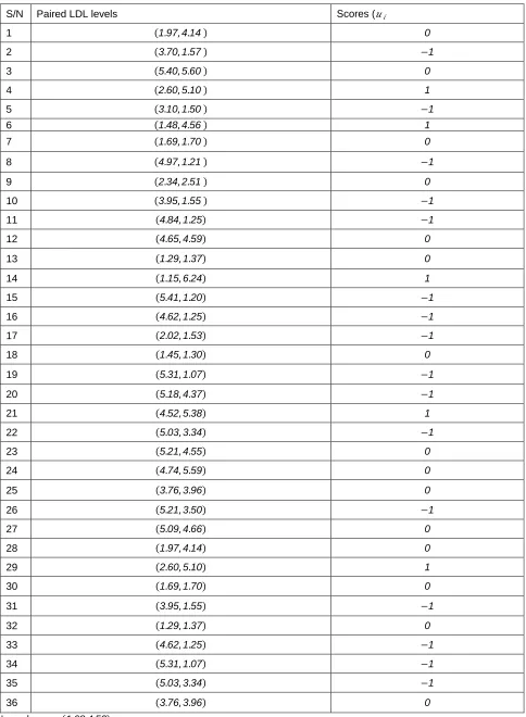
A medical researcher is interested in knowing the relationship between heart disease and low density lipo-protein levels (LDL). Using a random sample of 36 non-heart disease patients and another random sample of 36 heart disease patients, she paired each non heart disease
S/N Paired LDL levels Scores (𝑢𝑖
1 1.97,4.14 0
2 3.70,1.57 −1
3 5.40,5.60 0
4 2.60,5.10 1
5 3.10,1.50 −1
6 1.48,4.56 1
7 1.69,1.70 0
8 4.97,1.21 −1
9 2.34,2.51 0
10 3.95,1.55 −1
11 4.84,1.25 −1
12 4.65,4.59 0
13 1.29,1.37 0
14 1.15,6.24 1
15 5.41,1.20 −1
16 4.62,1.25 −1
17 2.02,1.53 −1
18 1.45,1.30 0
19 5.31,1.07 −1
20 5.18,4.37 −1
21 4.52,5.38 1
22 5.03,3.34 −1
23 5.21,4.55 0
24 4.74,5.59 0
25 3.76,3.96 0
26 5.21,3.50 −1
27 5.09,4.66 0
28 1.97,4.14 0
29 2.60,5.10 1
30 1.69,1.70 0
31 3.95,1.55 −1
32 1.29,1.37 0
33 4.62,1.25 −1
34 5.31,1.07 −1
35 5.03,3.34 −1
36 3.76,3.96 0
Applying the specification of Equation 26 to the LDL levels of Table 3 with 𝑐1 = 1.68, the lowest and 4.53 the highest
normal values respectively, we obtain the corresponding scores 𝑢𝑖of 1𝑠, 0𝑠 𝑎𝑛𝑑 −1𝑠shown in the 3𝑟𝑑 column of this table
Thus we have 𝑓+= 5, 𝑓0 = 15 𝑎𝑛𝑑 𝑓−= 16. Hence, we
have from Equations 11−13 that
𝜋 += 5
36= 0.139; 𝜋 0= 15
36= 0.417 𝑎𝑛𝑑 𝜋 −= 16
36= 0.444
From Equation14, we have that the estimated variance of
𝑊 𝐸𝑞𝑢𝑎𝑡𝑖𝑜𝑛 16 is
𝑉𝑎𝑟 𝑊 = 36 0.139 + 0.444 − −11 2
36 = 20.988 − 3.361 = 17.627
The null hypothesis to be tested is that heart disease patients and non-heart disease patients do not differ in their LDL levels which is equivalent to testing
𝐻0∶ 𝜋+− 𝜋−= 0 𝑣𝑒𝑟𝑠𝑢𝑠 𝐻1: 𝜋+− 𝜋−≠ 0
Using the test statistic of Equation 20 or 22, we have that
𝜒2= −11 2
17.627= 121
17.627= 6.864
𝑃 𝑣𝑎𝑙𝑢𝑒 = 0.0391
which with 𝑐 − 1 = 3 − 1 = 2 degrees of freedom is
statistically significant at only the 5 percent level 𝜒0.95,2 2 = 5.991 we may therefore conclude that heart disease patients and non- heart disease patients do infact differ in their LDL levels. The data of Table 2 may infact be represented by a 3𝑥3 table and following the specifications of Equation 26 with 𝑐1 = 1.68 𝑎𝑛𝑑 𝑐2= 4.53 to aid in clearer analysis as in Table 3
Table 4: Distribution of Scores 𝒖𝒊 of Matched pairs of case and control subjects of Table 3
Control 𝑇1 𝑆𝑐𝑜𝑟𝑒𝑠
Case 𝑇2 𝑆𝑐𝑜𝑟𝑒𝑠
Below Normal
𝑦𝑖1< 1.68
Normal
1.68 ≤ 𝑦𝑖1≤ 4.53
Above Normal
𝑦𝑖1> 4.53
Total
Below Normal
𝑦𝑖2< 1.68 4 0 2 6
Normal
1.68 ≤ 𝑦𝑖2≤ 4.53 5 6 3 14
Above Normal
𝑦𝑖2> 4.53 7 4 5 16
Total 16 10 10 36
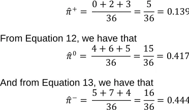
To re-analyse these data consistent with the generalized method, we have from Equation 11 that
𝜋 += 0 + 2 + 3
36 =
5
36= 0.139
From Equation 12, we have that
𝜋 0= 4 + 6 + 5
36 =
15
36= 0.417
And from Equation 13, we have that
𝜋 −= 5 + 7 + 4
36 =
16
36= 0.444
These are the same results obtained earlier using the scores in Table 3. We would therefore obtain the same values of 𝑊 −11 and chi-square 6.864 and arrive at the same conclusions. Hence, the present example illustrates how to analyse matched quantitative test scores without first converting them into frequency data. The data of
Example 2as presented in Table 4 may also be analysed using the Stuart/ Maxwell test. However as already pointed out, the Stuart/ Maxwell test statistic is atmost as powerful as the test statistic used in the proposed method presented here when the two methods are used with data of equal sample sizes
4.
Summary and Conclusion
[1]. Box GEP and Cox DR: A: An analysis of transformations. Journal of the Royal Statistical Society(B), 1964, 26, 211-252
[2]. Everitt BS. The analysis of contingency tables. London: Chapman and hall, 1977
[3]. Fleiss JL. Statistical Methods for Rates and Proportions (Second Edition) New York, Wiley 1981
[4]. Keefe TJ. On the relationship between two tests for homogeneity of the marginal distributions in a two-way classification. Biometrika, 1982, 69(3) 683-684
[5]. Maxwell AE: Comparing the classification of
subjects by two independent judges. British journal of Psychiatry, 1970, 116, 651-655
[6]. McNemar Q: Note on the sampling error of the difference between correlated proportions or percentages. Pychometrika 1947, 12, 153-157
[7]. Miettinen OS: Individual Matching with Multiple controls in the Case of all- or-more response. Biometrics, 1969, 22, 339-355
[8]. Robertson C, Boyle P, Hseih C, Macfarlane GJ,
and Maisonnesuve P: Some statistical
considerations in the analysis of case-control
studies when the exposure variables are
continuous measurement. Epidemiology, 1994, 5, 164-170
[9]. Schlesselman JJ: Case-Control Studies. New York:
Oxford University Press. 1992
[10]. Sheskin DJ: Handbbok of parametric and
non-parametric statistical procedures (second edition) Boca Raton Chapman and Hall, 2000, 491-508
[11]. Somes G. McNemar Test. Encyclopedia of
statistical sciences, S. kotz and N. Johnson, eds, , 1983, 5, 361-363. New York, Wiley
[12]. Stuart AA. A test for homogeneity of the marginal distributions in a two-way classification. Biometrika 1955, 42, 412-416