Modeling, Optimization and simulation of
Rotary Furnace using Artificial Neural
Network
Dr. R, K. Jain
Director, B.S.A. College of. Engineering and. Technology. MATHURA-281004(U.P) INDIA
Dr. D. K. Chaturvedi
Professor, faculty of engineering, D.E.I. Dayalbagh, AGRA-282005
Dr B. D. Gupta
Director Incharge, Anand Engg. College, Keetham, Mathura road, National highway, AGRA-
Abstract -This paper deals with modeling and simulation of LDO fired rotary furnace using feed forward modeling method of artificial neural network (ANN).The authors conducted experimental investigations on fuel consumption in a rotary furnace in an industry. It was observed that 6% oxygen enrichment of the air preheated up to 4600C simultaneously with reduction of air volume to 75% of its theoretical requirement lowered the specific fuel consumption to 0.260 lit/kg..The compact heat exchanger with 533 fins was used for preheating the air. Accordingly the emission level was also considerably reduced. The feed forward modeling method of artificial neural network contained in MAT LAB software was used for modeling and optimization of specific fuel consumption. The percentage variation, between actual experimental data and same data when simulated is +1.730%, and other feasible simulated datas is +6.192%,-3.038%,-5.692%,and+0.115%which is fairly acceptable.
Key Words – Rotary furnace, modeling, simulation, A.N.N. specific fuel consumption
1 Introduction [1],[2]-
Artificial neural networks are biologically inspired but not necessarily biologically plausible. Researchers are usually thinking about the organization of the brain when considering network configurations and algorithms. But the knowledge about the brain's overall operation is so limited that there is little to guide those who would emulate it. Hence, at present time biologists, psychologists, computer scientists physicists and mathematicians are working all over the world to learn more and more about the brain. Interests in neural network differ according to profession like neurobiologists and psychologists try to understanding brain, Engineers and physicists use it as tool to recognize patterns in noisy data, Business analysts and engineers use to model data, Computer scientists and mathematicians viewed as a computing machines that may be taught rather than programmed and Artificial Intelligentia, cognitive scientists and philosophers use as sub-symbolic processing (reasoning with patterns, not symbols) etc.
2 Method- modeling and simulation of rotary furnace [3] --The rotary furnace proved to be an eco-friendly and energy efficient furnace for ferrous foundries. The energy consumption measured in terms of specific fuel consumption has reduced significantly .The rotary furnace is a melting unit. The inputs parameters are divided in two groups-
(a) Independent parameters (b) Dependant parameters The Independent parameters are –
(1) Charge –fixed 200 kg (2) Fuel (liters)
(3) Preheated air volume (combustion volume)
(4) Oxygen consumption (oxygen supplied for combustion) These above parameters can be controlled by the operator The dependent parameters are –
(7) Preheated air temperature.
The Time required to melt charge of 200 kg depends upon fuel supplied, preheated air volume (combustion volume), and oxygen consumption (oxygen supplied for combustion).The flame temperature depends upon Fuel (liters), preheated air volume (combustion volume), preheated air volume (combustion volume).
The Preheated air temperature depends upon type of heat exchanger used, Fuel (liters), Preheated air volume (combustion volume), Oxygen consumption (oxygen supplied for combustion).These parameters are to be controlled during melting for minimum specific fuel consumption. In order to have an energy efficient furnace the specific fuel consumption should be minimum. It is shown in fig 1
INPUTS OUTPUT 1Charge- [fixed 200kg] ---
2Fuel (LDO) --- - Molten Metal
3Flame temperature --- 4Time / heat ---
5Preheated air volume --- 6Preheated air
temp---7Oxygenconsumption fig 1
3. Objectives-To minimize specific fuel consumption (lit/kg)--
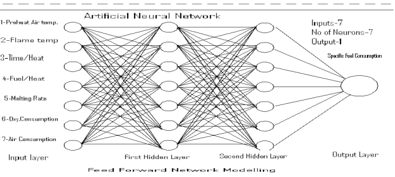
The rotary furnace datas used to train and test feed forward and back propagation neural networks have been extracted from actual experiments conducted on a 200 kg rotary furnace. A feed forward neural network model was developed to model the rotary furnace data.The ANN model uses seven inputs, two hidden layers of seven neurons (nodes) in addition to one node output layer. All input and output data’s are scaled so that they are confined to subinterval of 0-1.in this case each input or output parameter P is normalized as Pn before being applied to the neural network. The network as mentioned above has yielded comparatively better results. The network could predict output parameter with about 1-2% error. The results of tests are shown in following graphs. The conclusion from these experiments is that the tested network appears to constitute a workable model for modeling of rotary furnace parameters. The discrete structure is shown in fig.2.
Fig 2. Discrete structure of feed forward ANN model
4.Procedure followed [4] -The following procedure is adopted
A.N.N. modeling of rotary furnace parameters
(a)Selection of training and testing data- This is one of the most important and crucial part of ANN model development. If the training data is not appropriate sufficient and accurate, the ANN model output will not be good. For rotary furnace modeling using ANN the experimental data has been collected and 75% of it is used for training and rest 25% is used for testing. The data’s used for ANN model development are based on actual experimental investigations- effect of 6.9-% oxygen enrichment of 75.3%-75.4% of theoretically required air preheated up to 4600C, using compact heat exchanger, rotating furnace at optimal speed of 1.0 rpm, on flame temperature, time, fuel, melting rate, and specific fuel consumption as given in table.1- output is specific fuel consumption (column 8) which is to be reduced.
Table.1-Effect of 6.9-% oxygen enrichment of75.3%-75.4% of theoretically required preheated air on specific fuel consumption
(b)Normalization of Training data-The furnace was run for maximum preheated air temperature of 4600C,flame temperature 17550C, time required/heat 30.5 minutes, fuel required/heat 52 liters, melting rate 393.44 kg/hr, oxygen consumption/hea36.5m3,airconsumption /heat consumption/heat 426.5m3 which gave the specific fuel consumption of 0.260 liters/kg. The maximum limits of each input and output is selected .The inputs and respective output is divided by its maximum limit selected to normalize each of the inputs and output.
5Development of model
5.(1)Selection of suitable ANN structure The artificial neural network used in modeling of rotary furnace contains three layers, (seven input neurons, two layers of seven hidden neurons and one output neuron). This is developed in the Mat lab software ver. 7.2. The feed forward network back-propagation ANN model is developed and trained using normalized experimental data. Normalization is an important step in model development to give almost equal weight age to all the variables. To normalize the different input variable following maximum limits are taken respectively in same order. The maximum limit of output (specific fuel consumption) is 0.285 liter/kg. The absolute values of variables as per experimental data are divided by corresponding maximum limits .Maximum limits of inputs parameters are shown in table.2
SN Inputs Maximum limit
1 Preheat air temp 5000C
2 Flame temp 17600C,
3 Time required/heat 34 minutes 4 Fuel required 58 liters 5 Melting rate 400 kg/hr, 6 Oxygen consumption 40 m3 7 Preheated air consumption 460 m3
Table2- Maximum limits of inputs parameters
The maximum limit of output is shown in table.3
SN Output Maximum limit
1 Specific fuel consumption
0.285 liter/kg
Table.3- Maximum limit of output Sn Preheat
air temp ºc
Flame temp ºc
Time /heat min.
Fuel /heat lit.
Melting Rate kg/hr
Oxygen consump /heat m3
Air consump /heat m3
Specific fuel lit/kg.
5.(2) Training and development of model- Out of the seven (7) sets of observations of actual experimental datas as per table 6.1, only five sets have been selected for training and development of model.
5.(3) Test run of model –The model so trained and developed is tested for all seven sets of same table. Modeled specific fuel consumption based on above test run is compared with actual experimental specific fuel consumption.
5.(4) Simulation –For simulation different set of data’s (input parameters) are selected. The set of data’s selected are entirely different from experimental datas. 20 sets are used for simulation and average value of output is determined. 5.(5) Results–The results of simulation are tabulated and average simulated specific fuel consumption of each input parameter is compared. The optimum input simulated parameters are selected for minimum specific fuel consumption. 6. MODEL -The datas for training and development of model 1-6.9-% oxygen enrichment of 75.3%-75.4% of theoretically required air preheated up to 4600C, using compact heat exchanger, rotating furnace at optimal speed of 1.0 rpm, has been selected from. The input datas are-(a)preheated air temperature (b)flame temperature (c)time/heat (d)fuel/heat, (e)melting rate,(f)oxygen/heat and(g) air/heat
6.1 Selection of datas for training and development of model - Out of 7 sets of observations of table1only 5 sets have been selected for training and development as shown in table 4-
Heat no
Preheated air temp 0C
Flame temp. 0C
Time /heat. minutes Fuel /heat. liters Melting rate. kg/hr Oxygen cons. m3 Preheated air cons. m3
1 410.0 1710.0 33.00 56.0 363.0 39.0 459.0
2 418.0 1722.0 32.00 56.0 375.0 39.0 459.0
3 449.0 1746.0 31.50 54.0 385.0 38.0 443.0
4 454.0 1752.0 31.00 53.0 387.0 37.0 434.5
5 460.0 1755.0 30.50 52.0 393.4 36.5 426.5
Table 4 -The input datas selected for training and development of model l
The output (specific fuel consumption) corresponding to these inputs as per experimental data is given in table.5
Heat no 1 2 3 4 5
Specific fuel consumption lit/kg 0.280 0.280 0.270 0.265 0.260 Table 5 -Output (specific fuel consumption) corresponding to input datas selected
The normalized values of input datas selected for training and development of mode l as feed to ANN programme are shown in table 6
Heat no
Preheated air temp 0C
Flame temp. 0 C Time /heat minutes Fuel /heat liters Melting rate kg/hr Oxygen cons. m3 Preheated air cons. m3
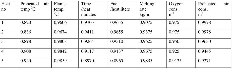
1 0.820 0.9606 0.9705 0.9655 0.9075 0.975 0.9978
2 0.836 0.9674 0.9411 0.9655 0.9375 0.975 0.9978
3 0.898 0.9808 0.9264 0.9310 0.9625 0.950 0.9630
4 0.908 0.9842 0.9117 0.9137 0.9675 0.925 0.9445
5 0.920 0.9859 0.8970 0.8965 0.9835 0.9125 0.9271
Table 6 -The normalized values of input datas selected for training and development of mode l
The normalized values of output (specific fuel consumption) corresponding to inputs as per experimental data is given in table.7
Heat no 1 2 3 4 5
Table.7- Normalized values of output (specific fuel consumption) corresponding to inputs
6.2 Programme for development of model - Mat lab
The ANN (Artificial neural network) programme contained in Mat lab is run as shown below- clc; clear all;
Close all;
%ip1=[410 418 449 454 460]; %ip1=[1710 1722 1746 1752 1755]; %ip1=[33 32 31.5 31 30.5]; %ip1=[56 56 54 53 52];
%ip1=[363 375 385 387 393.44]; %ip1=[39 39 38 37 36.5]; %ip1=[459 459 443 434.5 426.5];
%op=[0.9825 0.9825 0.9474 0.9123 0.9123]*.285; %p11=[410 418 428 449 454 458 460];
%p12=[1710 1722 1730 1746 1752 1754 1755]; %p13=[33 32 32 31.5 31 30.5 30.5];
%p14=[56 56 55 54 53 52 52];
%p15=[363 375 375 385 387 393.44 393.44]; %p16=[39 39 38.5 38 37 36.6 36.5];
p17=[459 459 451 443 434.5 426.7 426.5]; op=[0.280 0.280 0.2759 0.270 0.260 0.2609 0.260]; plot(p17,op)xlabel('Air/Heat.');ylabel('Specific fuel
6.3 The effect of individual input parameter on output (specific fuel consumption) - On basis of training and development of model l the effect of individual input parameter on output (specific fuel consumption) is shown in the following figures –
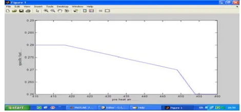
(1)Effect of preheated air temperature on specific fuel consumption is shown in fig.3
Fig3 Effect of preheated air temperature on specific fuel consumption-model (2)Effect of flame temperature on specific fuel consumption is shown in Fig4-
Fig 4 Effect of flame temperature on specific fuel consumption-model
Fig 5 Effect of time/heat on specific fuel consumption-model
(4)Effect of fuel/heat on specific fuel consumption is shown in fig6
Fig 6 Effect of fuel/heat on specific fuel consumption-mode
(5)Effect of melting rate on specific fuel consumption- is shown in fig.7
Fig7 Effect of melting rate (kg/hr) on specific fuel consumption-model
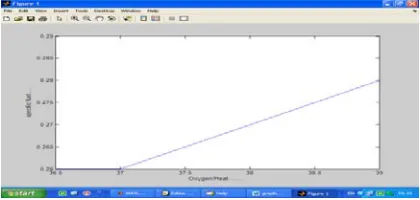
(6)Effect of oxygen/heat on specific fuel consumption- is shown in fig 8
Fig 9 Effect of air/heat on specific fuel consumption-model
The output parameter (specific fuel consumption) of model during training are given in table.8 Heat
no
Specific fuel consumption. lit/kg
1 0.280 2 0.280 3 0.270 4 0.260 5 0.260
Table.8- output parameter (specific fuel consumption) of model during training
6.4 Test run of model - The model 1 so trained and developed is being tested for its validity. The model is tested for all seven sets of observations as per table 6.1. In above programme rows p11 to p17corresponds to testing of model 1
6.4.1 On basis of test run of model - The effect of individual input parameter on output (specific fuel consumption) the effect of individual input parameters on output (specific fuel consumption) is shown in following figures –
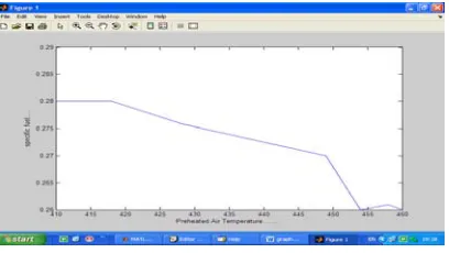
(1)Effect of preheated air temperature on specific fuel consumption—is shown in fig.10
Fig.10. Effect of preheated air temperature on specific consumption as per test run model
Fig 11- Effect of flame temperature on specific fuel consumption as per test run of model
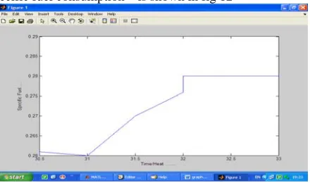
(3)Effect of time/heat on specific fuel consumption—is shown in fig 12
Fig 12- Effect of time/heat on specific fuel consumption
(4)Effect of fuel/heat on specific fuel consumption—is shown in fig 13
fig 13
Fig 14 Effect of melting rate (kg/hr) on specific fuel consumption
(6)Effect of oxygen/heat on specific fuel consumption is shown in fig.15
Fig 15- Effect of oxygen/heat on specific fuel consumption as per test run of model1
(7)Effect of air/heat on specific fuel consumption- is shown in fig 16
Fig 16 Effect of air /heat on specific fuel consumption as per test run of model1
On basis of test run of model1, the modeled output (specific fuel consumption) corresponding to inputs, is shown in table9
Table.9- The modeled output specific fuel consumption corresponding to inputs
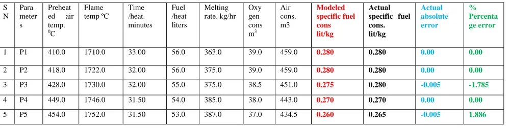
7.Comparison of outputs for model
The output (modeled specific fuel) consumption) of above test run of model1 are compared with actual specific fuel consumption and shown in table 10
S N
Para meter s
Preheat ed air temp. 0
C
Flame temp ºC
Time /heat. minutes
Fuel /heat liters
Melting rate. kg/hr
Oxy gen cons m3
Air cons. m3
Modeled specific fuel cons lit/kg
Actual specific fuel cons. lit/kg
Actual absolute error
% Percenta ge error
1 P1 410.0 1710.0 33.00 56.0 363.0 39.0 459.0 0.280 0.280 0.00 0.00
2 P2 418.0 1722.0 32.00 56.0 375.0 39.0 459.0 0.280 0.280 0.00 0.00
3 P3 428.0 1730.0 32.00 55.0 375.0 38.5 451.0 0.275 0.280 -0.005 -1.785
4 P4 449.0 1746.0 31.50 54.0 385.0 38.0 443.0 0.270 0.270 0.00 0.00
5 P5 454.0 1752.0 31.50 53.0 387.0 37.0 434.5 0.260 0.265 -0.005 1.886
Heat no 1 2 3 4 5 6 7
Specific fuel consumption lit/kg
6 P6 458.0 1754.0 30.50 52.0 393.4 36.6 426.7 0.2609 0.260 0.00 0.00
7 P7 460.0 1755.0 30.50 52.0 393.4 36.5 426.5 0.260 0.260 0.00 0.00
Table 10. – The comparison of output (modeled specific fuel consumption) of above test run of model 1 with actual specific fuel consumption
8Results-
The error between actual and modeled specific fuel consumption of model 1 varies between -1.785% to-1.886%.The average variation is -0.52%.It lies within acceptable limits of ±10%.
9. Presentation of error The error is presented, using Mat lab in fig. 17 clc;
clear all;
close all x=[0 0 -0.005 0 -0.005 0 0];y=erf(x) plot(y)
Fig17 -The errorbetween actual and modeled specific fuel consumption of model 1
10. Conclusions-
The maximum percentage error between modeled and experimental specific fuel consumption is -1.785%. The average variation is -0.524%. It lies within permissible limits of ±10%. Hence is acceptable.
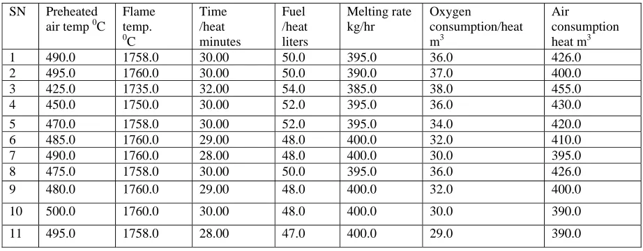
11. Simulation of output (specific fuel consumption)
For simulation, of output (specific fuel consumption), the different values of input parameters have been selected as shown in table 11-
SN Preheated air temp 0C
Flame temp. 0
C
Time /heat minutes
Fuel /heat liters
Melting rate kg/hr
Oxygen
consumption/heat m3
Air consumption heat m3
1 490.0 1758.0 30.00 50.0 395.0 36.0 426.0
2 495.0 1760.0 30.00 50.0 390.0 37.0 400.0
3 425.0 1735.0 32.00 54.0 385.0 38.0 455.0
4 450.0 1750.0 30.00 52.0 395.0 36.0 430.0
5 470.0 1758.0 30.00 52.0 395.0 34.0 420.0
6 485.0 1760.0 29.00 48.0 400.0 32.0 410.0
7 490.0 1760.0 28.00 48.0 400.0 30.0 395.0
8 475.0 1758.0 30.00 50.0 395.0 36.0 426.0
9 480.0 1760.0 29.00 48.0 400.0 32.0 400.0
10 500.0 1760.0 30.00 48.0 400.0 30.0 390.0
12 490.0 1758.0 30.00 50.0 395.0 36.0 426.0
13 460.0 1755 30.50 52.0 393.44 36.5 426.5
Table 11- The different values of input parameters
11.1 Programme of Simulation - The programme was run as shown below. The output is determined clc
close all clear all
% Tph TFlame Time fuel melting sp.fuel O2 Air x=[410 1710 33 56 363 0.280 39 459; 418 1722 32 56 375 0.280 39 459; 449 1746 31.5 54 385 0.270 38 443; 454 1752 31 53 387 0.260 36.60 426.7; 460 1755 30.5 52 393.44 0.260 36.50 426.5] T=[x(:,6)/0.285]'
P=[x(:,1)/500,x(:,2)/1760,x(:,3)/34,x(:,4)/58,x(:,5)/400,x(:,7)/40, x(:,8)/460]';
net = newff([0 1;0 1;0 1;0 1;0 1; 0 1;0 1], [7 1], {'tansig' 'purelin'}); net.trainParam.epochs = 500;
net = train(net,P,T); p1=P';
%r1=[490/500,1758/1760,30/34,50/58,395/400,36/40,426/460]'; %r2=[495/500,1760/1760,30/34,50/58,390/400,37/40,400/460]'; %r3=[425/500,1735/1760,32/34,54/58,385/400,38/40,455/460]'; %r4=[450/500,1750/1760,30/34,52/58,395/400,36/40,430/460]'; %r5=[470/500,1758/1760,30/34,52/58,395/400,34/40,420/460]'; %r6=[485/500,1760/1760,29/34,48/58,400/400,32/40,410/460]'; %r7=[490/500,1760/1760,28/34,48/58,400/400,30/40,395/460]'; %r8=[475/500,1758/1760,30/34,50/58,395/400,36/40,426/460]'; %r9=[480/500,1760/1760,29/34,48/58,400/400,32/40,400/460]'; %r10=[500/500,1760/1760,30/34,48/58,400/400,30/40,390/460]'; %r11=[495/500,1758/1760,28/34,47/58,400/400,29/40,390/460]'; %r12=[490/500,1758/1760,30/34,50/58,395/400,36/40,426/460]'; %r13=[460/500,1755/1760,30.50/34,52/58,393.44/400,36.5/40,426/460]' Y=sim(net,r12)
Y=sim(net,r13) Y1=Y*0.285
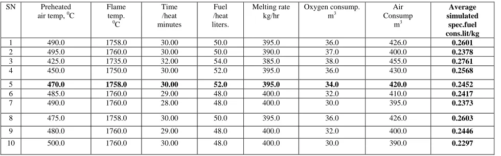
o/p=[0.2601,0.2378,0.2761,0.2568,0.2452,0.2417,0.2373,0.2603,0.2446 0.2297,0.2142, 0.2506, 0.2645] 12.Results of simulation--- the results of above simulation are shown in table 12
SN Preheated air temp, 0
C
Flame temp.
0 C
Time /heat minutes
Fuel /heat liters.
Melting rate kg/hr
Oxygen consump. m3
Air Consump
m3
Average simulated spec.fuel cons.lit/kg
1 490.0 1758.0 30.00 50.0 395.0 36.0 426.0 0.2601
2 495.0 1760.0 30.00 50.0 390.0 37.0 400.0 0.2378
3 425.0 1735.0 32.00 54.0 385.0 38.0 455.0 0.2761
4 450.0 1750.0 30.00 52.0 395.0 36.0 430.0 0.2568
5 470.0 1758.0 30.00 52.0 395.0 34.0 420.0 0.2452
6 485.0 1760.0 29.00 48.0 400.0 32.0 410.0 0.2417
7 490.0 1760.0 28.00 48.0 400.0 30.0 395.0 0.2373
8 475.0 1758.0 30.00 50.0 395.0 36.0 426.0 0.2603
9 480.0 1760.0 29.00 48.0 400.0 32.0 400.0 0.2446
11 495.0 1758.0 28.00 47.0 400.0 29.0 390.0 0.2142
12 490.0 1758.0 30.00 50.0 395.0 36.0 426.0 0.2506
13 460.0 1755.0 30.50 52.0 393.44 36.5 426.5 0.2645
Table 12 – The results of above simulation.
13. Comparison of experimental and simulated results-
The comparison of experimental and simulated results is shown in table 13
S N Parameters Preheated airtemp, 0 C
Flame temp. 0 C Time /heat min. Fuel /heat liters Melting rate kg/hr Oxygen cons m3 . Air Cons. m3 . specific fuelconslit/kg
1 Experimental 460.0 1755.0 30.5 52.0 393.44 36.50 426.5 0.260
2 Simulated (Experimental.)
460.0 1755.0 30.5 52.0 393.44 36.50 426.5 0.2645
3 Simulated (a) (Feasible) (b) (c) (d) 425.0 450.0 470.0 475.0 1735.0 1750.0 1758.0 1758.0 32.0 30.00 30.0 30.0 54.0 52.0 52.0 50.0 385.0 395.0 395.0 395.0 38.0 36.0 34.0 36.0 455.0 430.0 420.0 426.0 0.2761 0.2521 0.2452 0.2603
4 Simulated theoretical 500.0 1760.0 30.00 48.0 400.0 30.0 390.0 0.2297
Table 13- The comparison of experimental and simulated results.
14. Optimal Results—
The optimum values of input parameters for optimum specific fuel consumption, using feed forward method, is shown in table 14
Preheat air temperature0C
Flame temperature 0C
Time /heat min. Fuel /heat liters. Melting rate kg/hr Oxygen consumpti-on m3 Air consumpti-on m3
Specific Fuel consumption lit/kg
470.0 1758 30.0 52.0 395.0 34.0 420.0 0.2452
Table 14- The optimum values of input parameters for optimum specific fuel consumption
15. The percentage variation in experimental and simulated results-The percentage variation in experimental and simulated results is shown in table 15-
S N
Parameters Preheated air temp,0C
Experimental specific fuel cons. lit/kg
Simulated Specific fuel cons. lit/kg
Percentage variation
1 Experimental 460.0 0.260 0.260 ---
2 Simulated (Experimental.)
460.0 --- 0.2645 +1.730%
3 Simulated (a) (Feasible) (b) (c) (d) 425.0 450.0 470.0 475.0 --- 0.2761 0.2521 0.2452 0.2603 +6.192% -3.038% -5.692% +0.115 %
Table 15 -The percentage variation in experimental and simulated results
16. Remarks –
The maximum preheated air temperature which can be achieved by existing compact heat exchanger is 475-476 0
17. Conclusions-
The variation between actual experimental and simulated specific fuel consumption for(1) Same input parameters is +1.730%(2) For other feasible operating parameters is-5.692% to +6.192%%. It lieswithin acceptable limits of ±10%.hence simulation is acceptable
18. Acknowledgement:
The authors gratefully acknowledge the inspiration provided to them by Shri Harbhajan Singh Namdhari, proprietor, M/s Harbhajan Singh Namdhari Enterprises, Agra for not only permitting but also extending all cooperation and guidance during experimental investigations carried out on a 200 kg LDO fired rotary furnace installed in his foundry shop.
19. Reference list
[1] Karunakar D.B.Dutta G.L “Modeling of cupola furnace parameters using artificial neural networks” Indian foundry journal vol 48, no 5, may 2002 pp 29-39.
[2] Haykins Symon “Neural Networks” (text book) Pearson prentice hall, pp139-197
[3] Jain R.K., Singh R,. “Modeling and optimization of rotary furnace parameters using Regression & Numerical Techniques” 68th world Foundry Congress, Feb 7-10, 2008, Chennai