AFFINE INVARIANT OF 3D OBJECTS USING STATISTICAL AND ALGEBRAIC COEFFICIENTS

AFFINE INVARIANT OF 3D OBJECTS

USING STATISTICAL AND

ALGEBRAIC COEFFICIENTS

Elhachloufi Mostafa

University Cady Ayyad , Faculty Semlalia , Department of Informatics Marrakech, Morocco,

El Oirrak Ahmed

University Cady Ayyad , Faculty Semlalia , Department of Informatics Marrakech, Morocco,

Aboutajdine Driss

University Mohamed V, Faculty of Science, Department of physique LEESA-GSCM, BP 1014, RABAT

KADDIOUI MOHAMED NAJIB

University Cady Ayyad , Faculty Semlalia , Department of Informatics Marrakech, Morocco

Abstract : The increasing number of objects 3D are available on the Internet or in specialized databases and require the establishment of methods to develop description and recognition techniques[1,2,3] to access intelligently to the contents of these objects . In this context, our work whose objective is to present an affine invariants methods [4,5] of 3D objects .

The proposed methods based on the extraction of statistical and algebraic coefficients from the 3D object, these coefficients remain invariant against affine transformation of the 3D object. In this work, the 3D objects are transformations of 3D objects by one element of the overall transformation. The set of transformations considered here is the general affine group. The measure of similarity between two descriptor vector objects is achieved by a similarity function using the euclidean distance..

Keywords: Affine Invariants, 3D Objects, Statistical and Algebraic Coefficients, Affine transformation

1. Introduction

With the advent of the Internet, exchanges and the acquisition of information, description and recognition of 3D objects have been as extensive and have become very important in several domains. On the other hand, the size of 3D objects used on the Internet and in computer systems has become enormous, particularly due to the rapid advancement technology acquisition and storage which require the establishment of methods to develop description and recognition techniques to access intelligently to the contents of these objects.

In transform approaches a very rich literature emphasizes any interest in approaches based transform Haugh [14], [15] and [16] which consists in detecting different varieties of dimension (n-1) immersed in the space. In the same vein, this work focuses on defining methods for the description of 3D objects using statistical and algebraic coefficients.

2 Statistical Coefficients : The Canonical Correlation Coefficients

2.1 Representation of the 3D object

3D object is represented by a set of points denoted

 

1...

i _{i n}

M



P

_ where

P

_i



( ,

x y z

_{i j}

, )

_i



3 , arranged in a matrix

X

. Under the action of an affine transformation, the coordinates

( , , )

x y z

are transformed into other coordinates

( , , )

x y z

  

by the following procedure:

3 3

:

( ( ), ( ), ( )) ( ) ( ( ), ( ), ( )) ( ( ), ( ), ( ))

f

X x t y t z t f X Y x t y t z t Y A X x t y t z t B

 

 _{ }



   



 

  

 

1

With

A



(

a

_{ij i j}

)

_{, 1,2,3} invertible matrix associated with the infinite, and

B

is a vector translation in



3 .

2.2 The canonical analysis of two vectors :

X

and

Y

Let

X





X X

₁

,

₂

,...,

X

_p



t and

(

₁

,

₂

,...,

)

t q

Y



Y Y

Y

are two vectors.

The principle of this analysis is to searsh at the first a couple of variables



V W

1

,

1



which

V

1





₁

X

j is a normalized linear combination of variables

X

j (

X

j is jth _{column of X) and} 1

1 k

W





Y

a normalized linear combination of variables

Y

k (

Y

k is kth column), such that

V

1 and

W

1 are correlated as possible, i.e.:

that maximizes the quantity available



₁



Corr V W

(

1

,

1

)

.

Then we searsh the normed pair



V W

2

,

2



where

V

2





₂

X

jas being a linear combination of

X

j uncorrelated to

V

1 , i.e :

1 2

12

(

,

)

0

V

Corr V V







 

2

, and

W

2





₂

Y

k linear uncorrelated to

W

1 i.e :

1 2

12

(

,

)

0

W

_{Corr W W}







 

3

, which

V

2 and

W

2are correlated as possible, i.e: maximizes the quantity available



₂



Corr V W

(

2

,

2

)

. And so on...

The canonical analysis product p of pairs of variables where s = 1, .., p .The variables

V

sis an orthogonal basis of the space generated by

X

j . The variables

W

sis an orthogonal space generated by

Y

k.

The couples



V W

s

,

s



, particularly the first of them, reflect the linear connections between two groups of initial variables. The variables

V

sare

W

s are called canonical variables. Their successive correlations

(

k

,

k

)

Corr V W

The canonical correlation coefficients

(



_{s s}

)

_1,...,pare invariant quantities over an affine transformation and are all equal to 1 in this case.

2.3 Results and evaluation

We consider two 3D objects

X

and

Y

related by an affine transformation (figure 1 and 2). The calculation of canonical correlation coefficients from these objects requires computing the first pairs of canonical variables



s

,

s



_1,...,

s p

V W

 of

X

and

Y

then the coefficients of canonical correlations

(



s s

)

1,...,p from these couples. Figure 4 shows that the values of canonical correlation coefficients are all equal to 1. In another, Figures 5 shows that the canonical variables of origin objects and its transformation are the same which leads us to conclude that

Y

is an affine transformation of

X

according to the procedure of canonical analysis.

3. Algebraic Coefficients : Barycenter Coefficients

3.1 Genetic algorithms

Genetic algorithms (GA) were originally developed by John Holland [17].

They are used in order to find a solution, usually numerical solving of a given problem, without having a prior knowledge on the search space[18].

The basic structure of the genetic algorithm is as follows:  Creation of initial population

 Evaluation of adaptive function

While population numbers are less than maximum number of generations, do:  Generating new population

 Selection of best individuals  Generation progeny by crossing  Mutation of individuals

These algorithms are generally computationally implemented using genetic operation such as: •Creatingthe initial population: the production of initial population

•Coding: Consists of associates to each point of the state of space a data structure called chromosome •Selection: choose pairs of individuals surviving from one generation to another and those involved in the reproduction procedure of the future population

•Crossing: applies to two individuals randomly in the previous population. These individuals are matched to give birth to two offsprings

•Mutation: change randomly the value of the individual parameter 3.1.1 Operation parameters

The implementation of a genetic algorithm requires the adjustment of certain parameters: population size, survival rate, the mutation rate and number of generations as in any iterative algorithm, we must define a stopping criterion, a maximum number of iterations or detection of an optimum.

Fig 1.Representation of the canonical correlation coefficients

3.1.2 Learning and Simulation

Learning by genetic algorithm involves the evaluation of the behavior of each individual before generating new individuals who will in turn be evolved. In our case the individuals are the coefficients of barycenter.

3.2 Neural networks

Neural networks are very robust tools; they are widely used in pattern recognition, classification and knowledge representation [19].

In this network, neurons are arranged in layers. There is no connection between neurons of one layer, and connections made only with layers of swallow neurons.

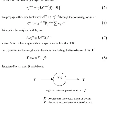
Usually, each neuron of one layer is connected to all neurons of the next layer and to it only. In our network, weights are first initialized with random values. Then the network receives the input vector. The output of this network is the vector. The objective is to determine the weights and biases which are represented respectively by



_p and



_p which transforms

X

into

Y

. For this, the signal is propagated forward in the layers of the neural network

X

_k(n1)



X

( )_jn

Y

_k(n1)



Y

_j( )n . The forward spread is calculated using the activation function g , the aggregation function h (often a scalar product between the weights and the inputs of neuron) and synaptic weight

w

_jkbetween the neuron

X

_k(n1) and the neuron

X

( )_jn , where :

( ) ( ) ( ) ( ) ( ) ( 1)

( )

n n n n n n

k j jk k

k

X  g h  g _ w X  _







 

4

When the forward propagation is complete, we get the output result R. We calculate the error between the output given by the R and the output vector desired T for this sample.

For each neuron i of output layer, we calculate :







i i



sortie i sortie

i

g

h

T

R

e



'



 

5

We propagate the error backwards

e

_i(n)



e

(_jn1)through the following formula:



( 1)



( ) )

1 ( ' ) 1

( n

i ij n

i n n

i g h w e

e    



 

6

We update the weights in all layers :

( )n ( )n (n1)

ij i j

w



e X







 

7

where



is the learning rate (low magnitude and less than 1.0).

Finally we return the weights and biases in concluding that transforms

X

to

Y

Y

  



X



 

8

designated by



and



as follows:

Fig 3. Extraction of parameters



and



X

:Represents the vector input of points

Y

: Represents the vector output of points

RN

3.3 Definition and properties of barycenter of an 3D object

3.3.1 Definition of 3D object barycenter

The barycenter of a 3D object is defined as follows:

3 3

( ) ( ) ( ) ( ) ( ) ( ) ( ) 1

1 2 1 2

1

:

( , , ..., ) ( , , ..., )

n

n X i i

X X X X X X i

n X n n

i i

f

a p

p p p g f p p p

a 



 

 

 _{  }

  





 



      

 

9

Where

p



_i(X)



( ,

x y z

_{i i}

, )

_i ,

g



_X



(

x

_G

,

y

_G

,

z

_G

)

and 1

0

n

i i

a







.

We note

CoefBary X

(

)



( ,

a a

_{1 2}

,...,

a

_n

)

barycenter coefficients of

g



_X

3.3.2 Properties of barycenter of

Y

i)The barycenter of

Y

(correspond to the 3D object) is defined as :

( )

1

1 n

Y i i i

Y n

i i

a p

g

a















 

10

ii)

g



c_Y

 



g



_X





 

11

where

g



_X is the barycenter of

X

.

Note:

CoefBary X

( )



CoefBary Y

( )



( ,

a a

_{1 2}

,...,

a

_n

)

.

3.4 Procedure for determining an affine invariant descriptive for 3D object

Given two objects 3D X and Y , for verifying that Y is an affine transformation of X, it suffices to verify that the barycenter coefficients of X and Y are equal, i.e.:

1 2

(

)

( )

( ,

,...,

_n

)

CoefBary X



CoefBary Y



a a

a

 

12

3.4.1 Calculation of the barycenter of X corresponds to the 3D object

According to the previous definition of barycenter we have:

( )

1 1

1 1

( , , )

( , , )

n n

X

i i i i i i

i i

X G G G n n

i i

i i

a p a x y z

g x y z

a a

 

 

 













1 1 1 1 1 1 n i i i G n i i n i i i G n i i n i i i G n i i a x x a a y y a a z z a                _       _   















1

1

( )

n

i i i i

i

G G G G n

i i

a x y z

x y z

a



       







1

1 n i i i G n i i

a

z

a



 







Where

i

x

i

y

i

z

i











1 1

(

)

n n

i G i i

i i

a



a



 









1 n

G i i

i

z

a











with 1

(

)

n

G i G

i

z

a











.

Then the problem amounts to determining the coefficients

( ,

a a

_{1 2}

,...,

a

_n

)

verifying the equation (4) where:

•



_iknown •

z



_Gunknown

Under our approach, we choose to use genetic algorithms to determine the barycenter coefficients of

g



_X.

3.4.2 Formulation of problem

Our problem is as follows: To determine the barycenter coefficients

( ,

a a

_{1 2}

,...,

a

_n

)

, we search to minimize a function

h a a

( ,

_{i 2}

,...,

a

_n

)

of this equation :

1 2

1

( ,

,...,

)

n

n i i

i

h a a

a

a









 

14

using genetic algorithms under the following constraint : 1

0

n i i

a







The result obtained by the genetic algorithm allows to determine the following coefficients

0 0 0

1 2

(

a a

,

,...,

a

_n

)

and

0

0 0 0

0

(

1

,

2

,...,

n

)

G

h



h a a

a



z



which led to calculate the barycenter :

0 0 0

1 1 1

0 0 0

1 1 1

(

,

,

)

,

,

n n n

i i i i i i

i i i

X G G G n n n

i i i

i i i

a x

a y

a z

g

x

y

z

a

a

a

     











































 

15

The next step is to prove if these coefficients are those of barycenter of Y .

For this, we must the first extract the parameters



and



from equation (8) and use it to calculate c

Y

g



( equation (11) ) , then we compare it with those obtained by equation (13) i.e. :

0 ( )

1 n Y i i i a p

g  





If the difference between the two barycenters

g



_Y and

g



_Yc ( error ) :

0

c

Y Y

err



g





g





 

17

isvery close to zero , then we conclude that the barycenter coefficients

(

a a

₁0

,

₂0

,...,

a

_n0

)

corresponds to X are those of barycenter of Y , i.e. :

0 0 0

1 2

(

)

( )

(

,

,...,

_n

)

CoefBary X



CoefBary Y



a

a

a

, consequently Y is an affine transformation of X .

3.5 Results and evaluation

Consider two 3D objects related by an affine transformation (figure 1 and figure 2). To calculate the vector of invariants from one of these objects, we calculate at first the coefficients of barycenter from one of two objects using genetic algorithms, secondly we extract the parameters



and



which can transform X and Y by neural network using it for calculate

g



c_Y.

Finally we compare the barycenter obtained by using coefficients barycenters previously calculated in

equation (12)

g



_Y and that obtained by using the parameters



and



extracted from the neural network as shown by equation (11)

g



c_Y.

The figure 4 and the figure 5 show that the two coefficients barycenters are equal. This leads us to conclude that the coefficients of a barycenter are invariant vectors for the two 3D objects.

4. Conclusion

I

n this work we presented the methods for affine invariants of 3D objects based on statistical and algebraic coefficients.

The first approach is based on canonical correlation coefficients obtained from the canonical analysis, this approach consists of extracting the canonical variables from the original object and its transformation, then we calculate their correlations, those are called canonical correlation coefficients, which are invariant quantities over an affine transformation.

The second approach relies on the extraction of barycenter coefficients from the 3D object using genetic algorithms and neural networks, these coefficients are invariant over an affine transformation of the object. Experimental results show the validity of these methods.

Fig 4. barycenter of the original 3D

object as function of its transformed Fig 5. L’erreur :

c

Y Y

References

[1] Ahmed El Oirrak, Mohamed Daoudi, Driss Aboutajdine: Affine invariant descriptors for color images using Fourier series. Pattern Recognition Letters 24(9-10): 1339-1348 (2003).

[2] Ahmed El Oirrak, Mohamed Daoudi, Driss Aboutajdine: Estimation of general 2D affine motion using Fourier descriptors. Pattern Recognition 35(1): 223-228 (2002).

[3] Ahmed El Oirrak, Mohamed Daoudi, Driss Aboutajdine: Affine invariant descriptors using Fourier series. Pattern Recognition Letters 23(10): 1109-1118 (2002)

[4] M. Petrou and A. Kadyrov. Affine invariant features from the trace transform. IEEE Transactions on Pattern Analysis and Machine Intelligence, 26(1):30{44, 2004.

[5] A. Choksuriwong, H. Laurent & B. Emile. A Comparative Study of Objects Invariant Descriptor. ORASIS, 2005.

[6] T. Murao, "Descriptors of polyhedral data for 313-shape similarity search", Proposal P177, MPEG-7 Proposal Evaluation Meeting, UK, Fév. 1999.

[7] M. Elad, A. Tal, S. Ar, "Directed search in a 3D objects database using SVM", Hewlett- Packard Research Report HPL-2000-20R1, 2000.

[8] C. Zhang, T. Chen, "Efficient feature extraction for 2D/3D objects in mesh representation", Proc. of the International Conference on Image Processing (ICIP 2001), 2001.

[9] T. Zaharia, F. Prêteux, "3D-shape-based retrieval within the MPEG-7 framework", Proc. SPIE Conf. on Nonlinear Image Processing and Pattern Analysis XII, Vol. 4304, pp. 133-145, San Jose, Etats-Unis, Janv. 2001.

[10] Taubin et D.B. Cooper, "Object recognition based on moment (or algebraic) invariants", J.L. Mundy and A. Zisserman, editors, Geometric Invariants in Computer Vision, pp. 375-397, MIT Press, 1992.

[11] S. J. Dickinson, D. Metaxas, A. Pentland, "The role of model-based segmentation in the recovery of volumetric parts from range data", IEEE Trans. on PAMI, Vol. 19, No. 3, pp. 259-267, Mars 1997.

[12] S. Dickinson, A. Pentland, S. Stevenson, "Viewpoint-invariant indexing for content- based image retrieval", Proc. IEEE Int. Workshop on Content-Based Access of Image and Video Database, pp. 20-30, Janv. 1998.

[13] J.W.H. Tangelder, R.C. Veltkamp, "Polyhedral model retrieval using weighted point sets", Rapport technique no UU-CS-2002-019, Universitd de Utrecht, Pays-Bas, 2002.

[14] P. V. C. Hough, "Method and means for recognizing complex patterns", U.S. Patent 3069 654, 1962.

[15] D. H. Ballard, "Generalizing the Hough transform to detect arbitrary shapes," Pattern Recognition, Vol. 13, No. 2, pp. 111-122, 1981.

[16] Illingworth et J. Kittler, "A survey of the Hough transform", Computer Vision, Graphics and Image Processing, Vol. 44, pp. 87-116, Oct. 1988.

[17] Lutton, E.Algorithmes génétiques et Fractales.Dossier d'habilitation à diriger des recherches, Université Paris XI Orsay, 11 Février 1999.

[18] Ludovic, Mé., Audit de sécurité par algorithmes génétiques. Thèse de Doctorat, Université de Rennes 1, France, 7 Juillet 1994. [19] R. LEPAGE, B. SOLAIMAN, Les réseaux de neurones artificiels et leurs applications en imagerie et en vision par ordinateur, Ecole