Using Transportation Model for Aggregate Planning:
A Case Study in Soft Drinks Industry
Suhada O. Tayyeh
*, Saffa J. Abdul-Hussien
Technical College of Management, Iraq
Abstract
In this paper, aggregate planning strategies are discussed and a special structure of transportation models are
investigated for the aggregate planning purpose of Baghdad Company for soft drinks. For the purpose of achieving the aims
of this study, we will develop an optimal total production plan by determining the quantities of production necessary to meet
the variable demand for a period of time in the medium term and at the lowest cost using the transportation model and then
comparing the company's plan with the proposed plan by adopting specific criteria for determining the best. The study
reached a set of conclusions, the most important of which is the development of an optimal production plan for the family of
the product under study for the year 2018, and recommended the need to work according to the optimal plan proposed, which
is better than the company's plan, since the total cost of production of the company and the unsold production cost of the
company, Is greater than the corresponding costs reached by the optimal solution of the transport model.
Keywords
Aggregate planning, Transportation model, Seasonal ARIMA, the bottom-up approach
1. Introduction
Aggregate production planning is concerned with
determining the quantity and timing of production in the
intermediate future to meet forecasted demand, it usually
covers a time period ranging from 3 to 18 months. The main
objective of aggregate planning is to minimize the total cost
over the planning horizon. The plan must take into account
the various ways a firm can cope with demand fluctuations as
well as the cost associated with them. Typically a firm can
cope with demand fluctuations by, changing the size of the
work force by hiring and firing (thus allowing changes in the
production rate), varying the production rate by introducing
overtime and (or) outside subcontracting, accumulating
seasonal inventories and planning backorders.
These ways of absorbing demand fluctuations can be
combined to create a large number of alternative production
planning options. Costs relevant to aggregate production
planning are basic production costs (material costs, direct
labor costs, and overhead costs), costs associated with
changes in the production rate and Inventory related costs.
There are two extreme aggregate production plans, the
just-in-time production plan and the production-smoothing
plan.
* Corresponding author:
[email protected] (Suhada O. Tayyeh) Published online at http://journal.sapub.org/logistics
Copyright©2018The Author(s).PublishedbyScientific&AcademicPublishing This work is licensed under the Creative Commons Attribution International License (CC BY). http://creativecommons.org/licenses/by/4.0/
of uncertainty. Jamalnia appraised also the performance of
different aggregate production planning strategies in
presence of uncertainty. Damghani etal. in 2017 proposed
a multi-period multi-product multi-objective aggregate
production planning (APP) model for an uncertain
multi-echelon supply chain considering financial risk,
customer satisfaction, and human resource training. They
considered three conflictive objective functions and several
sets of real constraints. Some parameters of the proposed
model are assumed to be uncertain and handled through a
two-stage stochastic programming (TSSP) approach. The
proposed TSSP is solved using the goal attainment technique,
the modified ε-constraint method, and STEM method. They
applied the whole procedure in an automotive resin and oil
supply chain as a real case study wherein the efficacy and
applicability of the proposed approaches are illustrated in
comparison with existing experimental production planning
method.
2. Statistical Tools
2.1. Seasonal ARIMA Model
SARIMA models are the most general class of models for
forecasting a time series, since there too many phenomena
that are follow to.. Seasonal ARIMA models are expressed in
factored form by the notation ARIMA(p,d,q)(P,D,Q)
s, where
p is the number of autoregressive terms, d is the number of
nonseasonal differences needed for stationarity, q is the
number of lagged forecast errors in the prediction equation, P
is the order of the seasonal autoregressive part, D is the order
of the seasonal differencing, Q is the order of the seasonal
moving-average process and s is the length of the seasonal
cycle.
Given a dependent time series
,
mathematically the ARIMA seasonal model is written as,
*
1 1
*
1 1
1
1
1
1
1
1
p P D
d
i S i S
i i t
i i
q Q
i S i
i i t
i i
C
B
B
B
B
y
B
B
e
(1)
where,
C
is a constant,
θ
’s and
Φ
’s are weighting parameters
for the different nonseasonal lagged terms,
θ
*’s and
Φ
*’s are
weighting parameters for the different seasonal lagged terms,
B is the back shift operator (
) and
e
represents a
random error term.
2.2. Transportation Model
This model can be used for a wide variety of situations
such as scheduling, production, investment, plant location,
inventory control and many others.
The transportation problem can be put in general form as
shown in table (1)
Table 1. Matrix of Transportation
Sources (Supply from)
Destinations (Demand for) Total supply (Capacity available)
B1 B2 … Bn
A1
s1
A2
s2
Am
sm
Total demand d1 d2 … dn
Where,
A
i– periods of production,
i
= 1,2, …,
m
(each period of
production may contains production in regular time,
production in overtime and production under subcontract),
(the beginning inventory may be taken as first period of
production)
B
j– periods of demand,
j
= 1,2, …,
n
m
– total number of containers produced
n
– total number of containers demanded
c
ij–unit costs for the transport between
i
-th period of
production and the
j
-th period of demand,
i
= 1,2, …,
m
,
j
= 1,2, …,
n
x
ij– number of containers supplied from
i
-th period of
production to
j
-th period of demand,
i
= 1,2, …,
m
,
j
= 1,2, …,
n
s
i– available number of produced containers at
i
-th period
of production,
i
= 1,2, …,
m
d
j– demand for containers at
j
-th period of demand,
j
=
1,2, …,
n
.
It is worth mentioning that the costs concluded the
regular production cost per unit, overtime cost per unit,
subcontracting cost per unit, holding cost per unit period,
Backorder cost per unit per period and inventory carrying
cost.
c
ijcontains some of costs which are compatible with
situation of
x
ij. The mathematical model for the solution of
the above transportation problem can be summarized as
follows:
Criteria function, Min
Z
=
1 1
m n ij ij i j
c x
with constraints,
i
n
j
ij
s
x
1
,
i
= 1,2, …,
m
(2)
j
m
i
ij
d
x
1
,
j
= 1,2, …,
n
(3)
x
ij≥ 0 ;
i
= 1,2, …,
m
,
j
= 1,2, …,
n
.
1 1
m n
i j
i j
s
d
.
There are some assumptions in the transportation model,
that are, total quantity of the item available at different
sources is equal to the total requirement at different
destinations, item can be transported conveniently from all
sources to destinations, the unit transportation cost of the
item of the item from all sources to destinations is certainly
and precisely known, the transportation cost on a given route
is directly proportional to the number of units shipped on that
route and the objective is to minimize the total transportation
cost.
The first step to solve transportation problem is to find out
the initial feasible solution. The Vogel approximation
method (VAM) is an iterative procedure for computing that
basic feasible solution. This method is preferred over the
other methods, because the initial basic feasible solution
obtained by this method is either optimal or very close to the
optimal solution. The steps in VAM are as follows,
1. Identify the boxes having minimum and next to
minimum transportation cost in each row and write the
difference (penalty) along the side of the table against
the corresponding row.
2. Identify the boxes having minimum and next to
minimum transportation cost in each column and write
the difference (penalty) against the corresponding
column
3. Identify the maximum penalty. If it is along the side of
the table, make maximum allotment to the box having
minimum cost of transportation in that row. If it is
below the table, make maximum allotment to the box
having minimum cost of transportation in that column.
4. If the penalties corresponding to two or more rows or
columns are equal, you are at liberty to break the tie
arbitrarily.
5. Repeat the above steps until all restrictions are
satisfied.
After computing an initial basic feasible solution, one can
used the modified distribution method (MODI) is for finding
the optimal solution of a transportation problem. It is
provides a minimum cost solution. The steps in MODI are as
follows,
1. Determine the values of dual variables, u
iand v
j, using
u
i+ v
j= c
ij2. Compute the opportunity cost using c
ij– ( u
i+ v
j).
3. Check the sign of each opportunity cost. If the
opportunity costs of all the unoccupied cells are either
positive or zero, the given solution is the optimal
solution. On the other hand, if one or more unoccupied
cell has negative opportunity cost, the given solution
is not an optimal solution and further savings in
transportation cost are possible.
4. Select the unoccupied cell with the smallest negative
opportunity cost as the cell to be included in the next
solution.
6. Draw a closed path or loop for the unoccupied cell
selected in the previous step. Please note that the right
angle turn in this path is permitted only at occupied
cells and at the original unoccupied cell.
7. Assign alternate plus and minus signs at the
unoccupied cells on the corner points of the closed
path with a plus sign at the cell being evaluated.
8. Determine the maximum number of units that should
be shipped to this unoccupied cell. The smallest value
with a negative position on the closed path indicates
the number of units that can be shipped to the entering
cell. Now, add this quantity to all the cells on the
corner points of the closed path marked with plus
signs, and subtract it from those cells marked with
minus signs. In this way, an unoccupied cell becomes
an occupied cell.
3. Case Study
To determine the optimal aggregate production plan, this
will be according to the following subsections,
3.1. Prepare the Necessary Data
The data needed to achieve the aims of the study will be
prepared as follows:
1. For the purpose of conducting quantitative analysis
appropriate to the objectives of the study, the monthly
data for the demand and production of 250 ml (Pepsi,
Miranda, Seven up, Green apple, peace, Shani, Lemon)
for the period from the beginning of 2012 until the end of
2017 was obtained from Baghdad Company of soft
drinks. This data is shown in tables (1-2) in annex
respectively.
2. Through the personal interview with the director of
production operations and the administrator of the first
line of production in Dijla plant, we learned that there are
two of works shift, the first one starts from seven in the
morning and ends at three in the afternoon (eight hours)
and then extend for another two hours as an additional
time until 5 pm. The second shift of the work begins from
7 pm to 3 am, followed by two additional working hours
until 5 am. It is also worth mentioning that:
a. The work shifts in Both of Fridays and Saturdays
treated as additional shifts.
b. Work is continuing for all days of the week except
public holidays approved by the government and
those granted to certain necessities. Table (3) In
annex shows these holidays over the months from the
beginning of 2012 until the end of 2017.
3. Based on Table (3) In annex, the actual and additional
working hours are in Table (4) In annex, were calculated
for January 2012, for example, as follows:
Saturdays plus an official holidays) 1 day of january
(1 January) Remaining 22 days, 31 - 8 - 1 = 22.
b. The additional working days (overtime) are (the
number of Fridays and Saturdays, which is 8 days,
minus a public holiday on Friday, (6th of January),
which will be 8 - 1 = 7.
c. The regular working hours are equal to the number of
regular working days of 22 days multiplied by 16
hours (8 working hours for each shift), (22 x 16 =
352).
d. The number of working hours for overtime is equal
to the number of regular working days of 22 days
multiplied by 4 hours (2 extra hours for each shift)
plus 7 overtime days multiplied by 20 hours (10
overtime hours in each shift) (22 x 4) + (7 x 20) = 228.
And so on for the rest of the months in the period
under study from the beginning of 2012 until the end
of 2017.
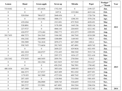
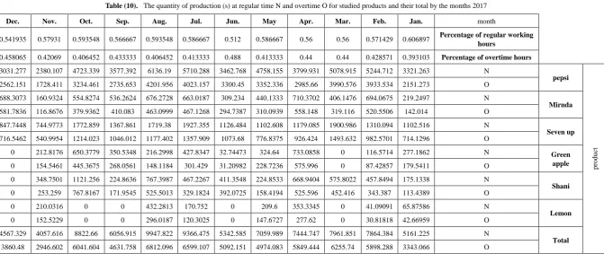
4. According to table (4) In annex, we calculated the
quantities of production within the regular and overtime
hours of each of the products under study. These
quantities are shown in tables from (5-10) In annex. for
example, for December 2012, the calculations are as
follows:
a. The ratio of the number of regular work hours to the
total number of working hours is, 352 / (580) =
0.606897.
b. We multiply the above ratio by the number of
containers produced of Pepsi in December 2012, the
production quantity in regular time is, 0.606897 ×
2199.327 = 1334.764.
c. The ratio of the number of overtime hours to the total
number of working hours is
228 / (580) = 0.393103.
d. We multiply the above ratio by the number of
containers produced of Pepsi in December 2012, the
production quantity in overtime is, 0.393103 ×
2199.327 = 864.5631. And so on for the rest of the
months and products for the period from 2012 to
2017.
It is worth mentioning that the single container contains
110 boxes, each box contains 30 metal cans of 250 ml.
3.2. Demand and Production Forecasts
For the purpose of planning the aggregate production of
the products of Baghdad Company for soft drinks and
specifically for 250 ml metal cans for the period from March
to December of 2018, firstly we will forecast the demand for
those products as well as the quantities of production at the
regular and overtimes in those months according to the
following steps:
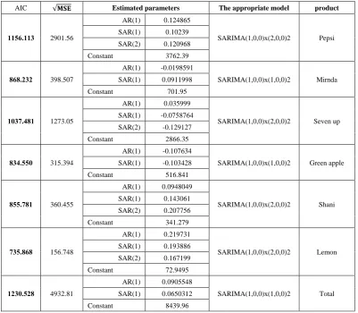
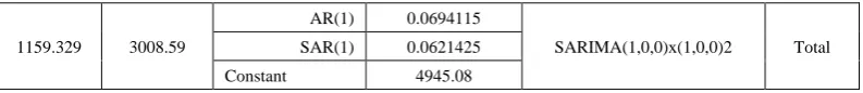
1. Based on the demand data in Table (1) In annex and the
quantities of production within the regular and overtimes
in Tables (5-10) In annex, the Akaike criterion was used
to determine the degree of appropriate model of data
among several estimated models. In addition, the root of
mean square error
is used to determine the
advantage of a model among several models were
estimated.
a. The models mentioned in Table (11) In annex, are
appropriate to represent the demand on containers for
each product, and then the total demand for the sum
of all products.
b. The models mentioned in Table (12) In annex, are
appropriate to represent quantities of production on
containers for each product within the regular time,
and then the total quantities of production for the sum
of all products.
c. The models mentioned in Table (13) In annex, are
appropriate to represent quantities of production on
containers for each product within the overtime, and
then the total quantities of production for the sum of
all products.
It should be noted that the criterion for selecting the
appropriate model is the least value of √MSE and the lowest
value of the AIC criterion, for example SARIMA (1.0,0) x
(2,0,0) 2, is a model which was chosen to represent demand.
It was used to forecast future values for Pepsi, with value of
√MSE equal to 2901.56 and value of Akiaki criterion equal
to 1156.113, which are the lowest among all corresponding
values of the models selected to represent the demand for
Pepsi product.
SARIMA (1,0,0) x (2.0.0) 2 model, which is represented
the demand on the Pepsi, can be written according to the
equation (1) as follows,
(4)
The parameters values listed in Table (6) are substituted in
the above equation to be,
–
(5)
by writing,
Equation (2) will be:
(6)
2. Before using the models mentioned in Tables (11-13) In
annex, for the purposes of forecasting, Box-Piers test
were used to confirm the ability of chosen models to
forecast. The Box-Piers test results that are shown in
Tables (14-16) In annex, indicate that the ability of
chosen models to forecast, where P value is the critical
point between accept and reject the hypothesis that the
model is able to forecast (there is no pattern for the
residuals). The rule is accept the hypothesis where the
chosen significant level is less than p. For example, p
value for demand model on Pepsi product is 0.765096,
Since this value is greater than all the common
significant levels 0.01, 0.05 and 0.10, we accept the
forecasts resulting from this model, and that the residuals
are random.
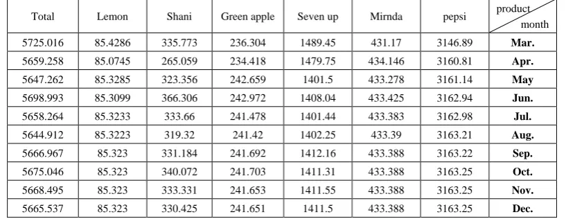
3. Using the models mentioned in Tables (11-13), the
forecasts for the demand for the products under
consideration, as well as the quantities of production at
the regular and overtime for the months from March to
December 2018, were obtained. Tables (17-19) In annex,
shows the values of these forecasts.
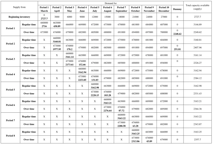
3.3. Using the Transportation Model
After obtaining the previous data and information related
with products under consideration beside the following
information,
1. Beginning inventory obtained from the company's
stores for each product are in table (2),
2. The production cost of single container in regular and
overtime are 660,000 Iraqi dinars and 673000
respectively (from the final accounts of the company).
3. The cost of storage of one container is 3000 Iraqi
dinars per month (from the company's accounts).
Table (2). Beginning inventory (containers) of the products under study on 1/3/2018
product Pepsi
Mirnda Seven
up Green
apple Shani Lemon
Beginning inventory 2727.7
279.2 1598.53 559.04
465.33 303
POM software was used to obtain the optimal value for the
costs resulting from satisfying the demand of the products
under consideration through the production of the company.
The Vogel method was used to get initial basic feasible
solution. The results are as follows,
1. product (Pepsi): Table (20) In annex, represents the
optimal solution for the transportation model. It is also
includes the data and information that represent the
analysis requirements to use the mentioned model. It
was found that the lowest optimal cost value is
34975750000 Iraqi dinar.
2. Product (Miranda): Table (21) In Annex, represents
the optimal solution for the transportation model. It
also includes the data and information that represent
the analysis requirements to use the mentioned model.
It was found that the lowest optimal cost value is
4850998000 Iraqi dinar.
3. Product (Seven up): Table (22) In Annex, represents
the optimal solution for the transportation model. It
also includes the data and information that represent
the analysis requirements to use the mentioned model.
It was found that the lowest optimal cost value is
15484670000 Iraqi dinar.
4. Product (green apple): Table (23) In Annex, represents
the optimal solution for the transportation model. It
also includes the data and information that represent
the analysis requirements to use the mentioned model.
It was found that the lowest optimal cost value is
2437385000 Iraqi dinar.
5. Product (Shani): Table (24) In Annex, represents the
optimal solution for the transportation model. It also
includes the data and information that represent the
analysis requirements to use the mentioned model. It
was found that the lowest optimal cost value is
3582915000 Iraqi dinar.
6. Lemon product: Table (25) In Annex, represents the
optimal solution for the transportation model. It also
includes the data and information that represent the
analysis requirements to use the mentioned model. It
was found that the lowest optimal cost value is
742554400 Iraqi dinar.
7. The sum of products: Table (26) In Annex, represents
the optimal solution for the transportation model. It
also includes the data and information that represent
the analysis requirements to use the mentioned model.
It was found that the lowest optimal cost value is
62074272400 Iraqi dinar.
3.4. Determination of Optimum Aggregate Production
Plan
In this section, we will discuss the results and determine
the aggregate production plan Proposed for each product and
for all products at once. For the purpose of arranging and
clarifying the results analysis, we will presenting it in
accordance with the following paragraphs,
1. Any company that wishes to sell all its production in
order to maximize its profits (equivalently, reduce its losses
due to the possibility of not selling part of its production).
Therefore, the Baghdad Company for soft drinks, when
produced at regular and overtime, assumes that all the
production will sold according to planned time. For this
purpose, we multiplied the production cost of the container at
the regular time which is 660000 iraqi dinar, by the quantity
of production at the regular time to obtain the production cost
at the regular time (row 1 in Table 3). We combined the
result with the cost of production in overtime (row 2 In Table
28) which is calculated by multiplying the production cost of
the container which is 673000 iraqi dinar, by the quantity of
production at overtime (row 3 in Table 3) (where the
company assumes that all of its production will be sold).
production of the single container at the regular time, which
is 660,000 Iraqi dinars, then the output will be about
20863220400 Iraqi dinars. This result represent the cost of
Pepsi product production at the regular time.
In addition, the forecasted production of containers of
Pepsi in overtime of the last ten months of 2018 is 23464.61
containers, which if it is multiplied by the cost of production
of the single container at overtime, which is 673,000 Iraqi
dinars, then the output will be about 15791682530 Iraqi
dinars. This result represent the cost of Pepsi product
production at overtime. By combining the above two results,
we get the total cost of Pepsi product production in the
company. Similarly, calculations are done for the other
company's products.
The POM software of Heizer's book was then used to
obtain the optimal solution (lowest possible cost) for each of
products under consideration and then for sum of all of them.
Row 4 in Table (3) includes this. The difference between the
cost of producing the product (for each product and the total)
and the cost calculated using the transport model is
mentioned in row (5). It is clear that the use of the transport
model to determine the optimal production cost is better than
the mechanism calculated by the company currently due to
the difference between the costs the products have total
aggregate.
For example, the difference between the cost calculated
according to the transportation model and the cost calculated
according to the company's mechanism of the Pepsi product
is 1679152930 Iraqi dinar. This amount represents a waste of
the company's money for the year under planning.
It should also be noted that the total cost of production
according to the company's mechanism is greater than the
cost calculated according to the transportation model,
although the total cost of production according to the
company's mechanism is multiplied by the cost of production
only (because the company usually assumes that all its
production will be sold without storage to reach the ideal
situation), while that the total cost calculated according to
transportation model multiplied by production cost plus
storage. This is due to the fact that the production of the
company is actually greater than the demand, which was
shown through the transportation model itself, as there was a
dummy column for the purpose of balancing production and
demand quantities, which contains unsold quantities of
production, which represent the difference between
production and demand.
Tables (20-26) In annex, show that there is a quantity of
production going to dummy demand column, which means
that the production is greater than the demand, which is
means also that the company bears the additional costs
resulting from the production of these quantities without real
demand. The explanation is the same for other products.
2. In the sixth row of Table (3), we find the cost of
non-sold production according to the company's mechanism,
which is calculated as follows for each product, by adding
the quantity of containers produced in the regular time to the
quantity of containers produced in overtime and quantity of
beginning inventory of production and then subtract the
demand from the result. Then the result multiplied by the
cost of production and storage, which is 700 thousand Iraqi
dinars. For example, for seven up product, the result is,
(10543.63 + 14228.95 + 1598.53 - 24879.34) × 700000 =
1044239000 Iraqi dinars.
The seventh row of table (3) includes the cost of unsold
production according to the optimal solution of the
transportation model. It is calculated by multiplying the cost
of production and storage by corresponding quantities of
unsold products in the dummy balance column. For example,
from the transportation table of the seven up product, the
quantities of unsold output are 1053.64, 431.26, 3.44 and
3.43 respectively of production in the overtime of the first,
second, third and fourth production periods. By multiplying
these quantities by corresponding production and storage
costs, we will obtain the cost of the unsold production of the
seven up product according to the optimal solution of the
transportation model as follows, 1053.64 (700000) +431.26
(697000) +3.44 (694000) +3.43 (691000) = 1042893710.
We note that the cost of unsold production of seven up
product according to the optimal solution of the
transportation model is less than the cost of production that is
unsold according to company's mechanism. The difference is,
1044239000 - 1042893710 = 1345290 Iraqi dinars. similarly,
calculations are done for the rest of the products and sum of
those products.
It is noted that the cost of production, that is unsold,
according to the optimal solution of the transportation model
is less than the corresponding cost according to company's
mechanism for each of products as well as the sum of those
products. row 8 of Table (3) includes the differences between
the costs.
3. In the ninth row of table (3), we find the losses of unsold
production according to company's mechanism, which is
calculated for each product as follows; the quantity of
containers produced in regular time plus the quantity of
containers produced in overtime plus quantity of containers
of beginning inventory minus the demand for that product,
then the result is multiplied by the cost of storage only, which
is (27000 dinars), for example, the losses for seven up
product will be, (10543.63 + 14228.95 + 1598.53 - 24879.34)
× 27000 = 40277790 Iraqi dinars.
It is worth mentioning that to calculate the loss, we
multiplied by the cost of storage only, on the basis that the
unsold production will be sold in the next year, 2019 as
beginning inventory.
Table (3). Production costs and losses according to company's mechanism and to the transportation model (in Iraqi dinar)
Sum
Product
Lemon Shani Green
apple Seven up Mirnda pepsi
37428434406 563032206 2163800760 1587927000 9391107000 2859347040 20863220400 production Cost at regular time () 1
28340889085 434200420 1640041776 1191036366 7095862990 2188065003 15791682530 production Cost at overtime ) 2(
65769323491 997232626 3803842536 2778963366 16486969990 5047412043 36654902930 Total production cost according to
company's mechanism )2(+)1(=)3(
62074272400 742554400 3582915000 2437385000 15484670000 4850998000 34975750000 optimal cost according to the
transportation model ) 4(
3695051091 254678226 220927536 341578366 1002299990 196414043 1679152930 )4(-)3(=)5(
3853963820 267115520 230776000 357179900 1044239000 204352400 1750301000
Cost of unsold production according to company's mechanism ) 6(
3846698830 264226640 230439020 355535230 1042893710 204058660 1749545570
Cost of unsold production according to according to transportation model ) 7(
7264990 2888880 336980 1644670 1345290 293740 755430 )6(-)7(=)8(
148652890 10303027 8901360 13776939 40277790 7882164 67511610
Losses of unsold production (inventory) according to company's mechanism ) 9(
141838464 7860000 8569764 12136980 38932500 7583040 66756180
Losses of unsold production according to optimal solution of the transportation model (inventory) (10)
6814426 2443027 331596 1639959 1345290 299124 755430 )9(-)11(=)11(
Table (4). The optimal aggregate production plan for the months from March to December 2018
Sum Product Production time Production periods Limon Shani Green apple Seven up Mirnda Pepsi
5690.9 51.32 335.77 236.3 1489.45 431.17 3146.89 regular time
1
42.65 42.65 Overtime
5659.292 85.087 265.06 234.435 1479.75 434.15 3160.81 regular time
2
3224.95 113.38 622.58 332.84 2156.15 Overtime
5647.27 85.33 323.36 242.66 1401.5 433.28 3161.14 regular time
3
3932.63 239.32 1051.11 315.93 2326.27 Overtime
5699 85.31 366.31 242.97 1408.04 433.43 3162.94 regular time
4
4231.75 278.17 186.59 1051.11 331.8 2384.08 Overtime
5658.26 85.32 333.66 241.48 1401.44 433.38 3162.98 regular time
5
4128.285 248.825 177.28 1054.51 316.24 2331.43 Overtime
5644.91 85.32 319.32 241.42 1402.25 433.39 3163.21 regular time
6
4208.08 57.76 233.17 172.3 1054.51 325.98 2364.36 Overtime
5666.96 85.32 331.18 241.69 1412.16 433.39 3163.22 regular time
7
4208.4 59.9 246.46 181.71 1054.51 321.96 2343.86 Overtime
5675.04 85.32 340.07 241.7 1411.31 433.39 3163.25 regular time
8
4234.893 59.5 253.91 183.72 1054.51 325.503 2357.75 Overtime
5668.49 85.32 333.33 241.65 1411.55 433.39 3163.25 regular time
9
4212.26 60.36 248.94 179.46 1054.51 322.4 2346.59 Overtime
5665.54 85.32 330.43 241.65 1411.5 433.39 3163.25 regular time
10
4215.803 60.17 245.053 178.42 1054.51 323.96 2353.69 Overtime
93315.36 1116.657 5385.718 3665.435 23280.81 7291.623 52575.12 optimal quantity of production that meet demand 5932.8 303 465.33 559.04 1598.53 279.2 2727.7 beginning inventory
For example, from the seven up transportation table, the
quantities of unsold containers of production are 1053.64,
431.26, 3.44 and 3.43 respectively of production in the
overtime of the first, second, third and fourth production
periods, these quantities are multiplied by the corresponding
storage cost, we will get the unsold production losses for
seven up product according to the optimal solution of the
transportation model,
1053.64 (27000) +431.26 (24000) +3.44 (21000) +3.43
(18000) = 38932500 Iraqi dinars.
We note that the unsold production losses of the seven
up product according to the optimal solution of the
transportation model are less than the unsold production
losses according to company's mechanism. The difference is,
40277790-38932500 = 1345290 Iraqi dinars. These
differences are positive for all products and then for their
sum. Row 11 in table (3) contains these differences.
4. Our main goal has been achieved, based on all of the
above, Baghdad Soft Drinks Company can adopt the
aggregate plan of production in Table (4) for all products
under consideration (Pepsi, Miranda, Seven up, Green Apple,
Shani, Lemon) and then their sum.
4. Conclusions, Recommendations and
Future Studies
Before stating the conclusions, it should be stated that,
1. The company is not designed an aggregate production
plan but it is put an estimated annual plan in the light
of achieved actual sales by using the method of the
seasonal exponential smoothing, which is one of the
simple forecasting methods. This plan is adopted for
production purposes.
2. The company did not specify the quantities of
production in the regular time and the overtime
required to meet the demand but the company adopted
the method of production and storage directly, this
leads to increase costs because of most of inventory
production will be from production in overtime,
without taking into account that need to meet the most
demand from production in the regular time, while the
remaining demand will be met from the production in
overtime. This mean that the inventory at the end of
the plan period must be zero or at least close to zero in
the optimal aggregate production planning.
3. The company did not specify from which Production
batches (periods) should meet the sequential monthly
demand so that costs are as low as possible.
4. The company bears a cost of storage higher than the
cost of the best plan (which is supposed to bear), since
the unsold production was used as a beginning
inventory in the beginning of the year.
Then, an aggregate total production plan for all the studied
products (Pepsi Cola, Miranda, Green apple, Seven up, Shani
and Limon) has been putted, and thus for their total sum of
250ml metal cans category, in both regular time and
overtime. production in 2018 under this plan fully covers the
forecasted demand, taking into consideration the beginning
inventory, since, it is well known that production is as much
as demand in an optimal aggregate production plan. Some of
the results of this optimal plan are as follows,
1. The total cost of production under the company's
mechanism for each product and then for the total sum
is greater than the cost reached according to the
optimal solution of the transportation model.
2. The cost of unsold production under the company's
mechanism for each product and then for the total sum
is greater than the unsold production cost reached
according to the optimal solution of the transportation
model.
3. Losses of unsold production (inventory) according to
the company's mechanism for each product and then
for the total sum is greater than the losses of unsold
production according to the optimal solution of
transportation model.
Based on the above, the bottom-up approach was used to
assemble the plans of the six products under consideration
to put the aggregate production plan. So, we are highly
recommended to work according to the proposed optimal
aggregate production plan.
As future studies, we suggest using the optimization
models along with an appropriate forecasting models to put
an aggregate production plan for other families of products
in Baghdad Soft Drinks Company and for other commodity
products of other companies, also for services sector such as
the health sector or Municipal sector. Also, we suggest
studying the relationship between the use of transportation
model to plan an aggregate production and achieve
competitive dimensions.
Appendix
Table (1). Actual demand on produced containers for products under study
Lemon Shani Green apple Seven up Mirnda Pepsi Product
Month Year
376.5273 0 625.1 2415.736 334.5273 3188.791 Jan.
2112
216.6091 0 400.3818 2361.2 961.4727 4119.927 Feb.
347.8818 0.109091 1023.245 3008.191 1232.245 3561.8 Apr.
203.5545 439.6364 0.836364 1913.736 684.8 4660.664 May
43.8 538.8091 0 3151.773 832.2091 3821.182 Jun.
0 227.9727 0 4880.227 793.3727 6201.118 Jul.
0 426.0727 1374.464 2975.582 729.1182 4325.591 Aug.
293.2727 406.7273 277.5455 3139.7 184.7545 4517.409 Sep.
0.472727 456.2182 311.7 2934.836 1086.255 5487.418 Oct.
0 327 619.2909 1654.209 750.9818 2499.909 Nov.
0 237.1818 220.7091 850.5182 96.36364 4189.173 Dec.
0 269 205.5727 2817.682 508.0091 4828.409 Jan.
2013
0 378.0182 394.6091 2712.918 595.4545 4188.936 Feb.
0 416.4636 444.2909 2604.8 565.8909 5219.409 Mar.
217.4545 534.0455 518.2 2061.536 718.3636 3307.564 Apr.
0.863636 184.3273 384.3364 840.3182 600.9727 3027.755 May
0 0 2.381818 583.6545 616.6909 1773.845 Jun.
348 641.2364 0.109091 3930.664 1095.027 4504.264 Jul.
132.1636 466.2909 217 4593.2 994.6273 6027.891 Aug.
0 1117.055 365.8909 3724.555 610.8727 6750.9 Sep.
0 269.3091 0.390909 2021.673 731.6091 5497.773 Oct.
0 588.4909 296 3568.391 538.3727 5339.209 Nov.
0 246 301 452.2091 213.4364 1186.773 Dec.
0 309.4091 32.6 948.9636 337.1273 5506.745 Jan.
2114
0 579.6455 636.0273 1529.255 404.0727 4316.264 Feb.
0 222.0273 302.6 1574.609 546.5091 2866.391 Mar.
0 465.6636 238.8636 1570.309 700.2818 2656.264 Apr.
0 736.9545 661.0091 4316.355 710.1818 6370.409 May
0 643.8636 292.0364 1803.927 538.8273 3569.755 Jun.
0 477.8545 7.672727 2242.864 611.0818 2886.718 Jul.
0 889.1818 708.8273 2744.282 756.6091 4744.627 Aug.
0 907.4909 582.9091 2916.655 1027.536 5837.836 Sep.
0 762.7818 599.0364 3138.155 875.1091 6024.427 Oct.
0 382.0182 336.7636 1770.345 447.1909 4600.118 Nov.
0 230.1545 25.18182 895.6 273.1818 1599.218 Dec.
Lemon Shani Green apple Seven up Mirnda Pepsi Product
Month Year
0 419.2364 503.9455 1451.227 595.0545 4172.036 Jan.
2015
248 541.3909 85.88182 2420.855 461.5091 4843.491 Feb.
207.2455 491.6545 660.7636 2114.227 779.9818 5079.564 Mar.
270.9182 518.1909 418.9273 2154.227 730.9 4427.327 Apr.
227.0545 631.7 452.0636 2449.564 725.2636 5549.145 May
373.1545 530.6364 447.5545 2437.291 683.4091 5161.527 Jun.
210.0364 594.5636 457.0818 2373.618 811.6455 5333.673 Jul.
369.4545 896.1364 611.3273 2542.418 1003.318 6641.418 Aug.
308.2636 734.2182 499.3636 2857.155 888.8091 6935.145 Sep.
274.0818 684.2 458.7273 2311.209 930.7455 5601.245 Oct.
90 329.6818 273 1605 464.9091 3481.7 Nov.
999.5727 2536.209 1873.6 9942.518 3104.745 23330.21 Dec.
118.0091 589.3545 200.4364 1824.155 654.4273 5182.427 Jan.
2016
178.0182 427.5 497.1273 1903.173 565.6 4876.145 Feb.
150.1182 706.4182 376.1727 2107.991 584.2364 5966.182 Apr.
293.0091 630.2364 439.0091 2852.682 1186.164 7373.791 May
378.3636 894.3909 630.4 2420.318 836.5909 6150.127 Jun.
349.4 1311.9 395.3545 3068.864 1340.155 8873.027 Jul.
278.9182 809.9727 552.0182 3173.309 1200.945 9114.691 Aug.
220.8 583.6091 594.5455 3240.864 619.8273 8758.8 Sep.
0 1078.718 401.0364 2586.373 892.2727 8705.891 Oct.
0 779.6364 0.009091 1101.973 982.5364 4934.173 Nov.
0 384.9364 460.8818 1225.818 372.9273 2729.255 Dec.
108 467.4091 572.7727 1727.209 465.5091 6078.382 Jan.
2017
72.03636 800.4636 202.0818 2416.436 1050.936 9121.1 Feb.
0.418182 1033.118 2.381818 3171.818 873.0727 9157.655 Mar.
333 675 955.1091 1770.618 806.7818 5145.164 Apr.
309.0091 799.5545 557.0091 2441.3 1024.836 9105.082 May
191 845.0455 292.0455 2098.209 607.1 7503.2 Jun.
218.2455 860.1273 682 3392.164 1240.045 9749.055 Jul.
321 1227.009 533.0091 2897.173 1180.091 10344.14 Aug.
280.5909 462.7091 619.5 2414.082 917.2818 5923.055 Sep.
146.7455 1285.036 722.0273 2768.691 1010.109 7581.618 Oct.
92.01818 591 387 1504.164 280.8273 4879.9 Nov.
86.26364 558 184 1403.955 982.5091 5611.564 Dec.
Source: Sales Department
Table (2). Actual production for produced containers
Lemon Shani Green apple Seven up Mirnda Pepsi Product
Month Year
733.0182 0 652.6636 1752.545 0 2199.327 Jan.
2112
0 0 0 2457.8 1233.864 4619.164 Feb.
0 520.0364 700.6727 2640.436 0 1726.736 Mar.
0 0 1013.082 3008.173 1298.355 3570.236 Apr.
0 439.6364 0 1913.691 675.7818 4658.491 May
0 538.8091 0 3178.309 1445.336 3820.136 Jun.
0 227.9727 0 4866.145 220.0455 6212.182 Jul.
0 426.0727 1374.464 2962.773 632.2273 4309.091 Aug.
293.7455 406.7273 294.3545 3184.382 184.7545 4518.209 Sep.
0 456.2182 294.8909 3200.009 1169.945 5502.5 Oct.
0 350.2909 726.1818 2070.273 667.2909 2492.6 Nov.
0 558.7455 773.6636 292.7455 487.4091 4859.745 Dec.
0 0 0 2650.227 429.9636 4421.955 Jan.
2013
0 402.1818 446.8727 2721.655 308.5182 3933.718 Feb.
0 459.2727 0 2597.273 1034.127 5521.418 Mar.
218.3182 575.5455 660.5455 2059.791 278.0364 3150.2 Apr.
0 0 182.2364 843.5455 547.5545 2914.227 May
0 0 0 658.2545 706.7091 1790.482 Jun.
480.1636 641.2364 0 3853.636 1098.955 4446.673 Jul.
0 466.3273 217.8727 4615.409 901.4182 6037.691 Aug.
0 1179.955 365.3909 4727.036 609.7545 6757.527 Sep.
0 207.1455 0 1156.964 731.4364 5481.655 Oct.
0 587.8545 296.0909 3650.745 538.6455 5332.918 Nov.
0 289.2727 333.5091 667.4091 304.5364 2586.936 Dec.
0 691.1091 764.1455 1105.327 307.0727 3304.164 Feb.
0 284.9091 294.4091 1884.273 331.6182 3347.582 Mar.
0 290.7 38.36364 1125.918 647.4273 2222.155 Apr.
0 928.3182 661.1273 4424.755 861.0091 6641.236 May
0 640.3091 299.6727 1862.509 367.6455 3456.682 Jun.
0 290.3273 0 2090.664 611.7091 3107.936 Jul.
0 994.3273 708.8364 2727.809 755.9818 4731.555 Aug.
0 810.8273 808.1818 2916.745 1076.6 5879.645 Sep.
19.03636 908.2636 512.7545 3301.027 982.2364 6174.9 Oct.
0 294.9091 222.8636 1865.673 311.7182 4004.073 Nov.
0 293.8818 0 805.3182 246.4636 2023.464 Dec.
Lemon Shani Green apple Seven up Mirnda Pepsi Product
Month Year
0 288.6273 589.8273 1482.455 693.5091 3737.582 Jan.
2015
0 549.7636 0 2334.773 533.0545 5055.482 Feb.
0 569.9636 849.5545 2426.055 747.4091 5602.7 Mar.
0 569.9182 393.1 2073.745 609.6 5027.545 Apr.
0 682.2182 402.9091 2664.118 840.3545 4950.745 May
0 363.8091 471.4091 2252.618 849 5401.927 Jun.
0 746.0727 518.2545 2403.691 581.1364 4734.573 Jul.
0 994.2273 584.6636 2716.973 1228.191 7568.664 Aug.
0 685.9636 513.9182 2698.9 874.0091 6178.136 Sep.
0 461.4636 293.6091 2067.7 678.9909 5521.591 Oct.
0 343.7727 439.4818 1428.564 648.5364 3014.045 Nov.
0 2508.855 1856.582 10060.11 2994.027 24477.23 Dec.
0 680.1455 59.2 1899.473 810.9909 4450.964 Jan.
2016
140.6273 400.8364 574.0364 2112.4 359.1727 5087.909 Feb.
292.6091 502.8727 424.0727 1655.745 913.5727 6224.882 Mar.
0 576.7091 221.1818 1862.527 359.6091 4756.827 Apr.
296.7273 749.1364 436.1091 3112.809 1344.209 8251.636 May
441.1091 992.1182 735.2545 2159.345 736.7364 6843.8 Jun.
5042.636 1156.6 290.4 3068.827 1282.018 7305.436 Jul.
0 654.3091 585.5636 3627.191 1233.764 9134.618 Aug.
220.7 537.5545 589 3263.7 611.0455 8124.736 Sep.
0 1077.345 401.3818 2549.155 888.4273 8738.473 Oct.
0 781.5 0 1269.482 1212.155 4909.982 Nov.
0 561.4909 577.0545 1098.791 239.4182 3458.782 Dec.
108.5455 288.5727 456.7273 1816.645 361.2636 5472.536 Jan.
2017
71.90909 801.2364 204 2292.664 1214.618 9178.245 Feb.
0 1028.218 0 3394.618 725.2636 9069.491 Mar.
630.9545 1194.536 1309.082 2105.509 1268.518 6785.591 Apr.
357.2727 383.2727 553.3636 1879.445 750.2273 8110.491 May
0 803.4273 63.95455 2200.164 603.9727 6763.218 Jun.
291.0545 796.4091 729.2636 3285.264 1130.145 9733.445 Jul.
728.3 1292.9 364.4182 2896.782 1139.373 10338.15 Aug.
0 396.8182 618.5909 2413.873 946.3455 6313.045 Sep.
0 1889.073 1095.745 2986.882 934.7636 7957.8 Oct.
362.5545 602.0091 367.3636 1285.973 277.8 4108.518 Nov.
0 0 0 1564.291 1270.091 5593.427 Dec.
Table (3). Public holidays over the period studied 2012-2017
No. holidays in which there is no work
No. Fridays and Saturdays
No. days Year
No. holidays in which there is no work
No. Fridays and Saturdays
No.
days month Year
3 8 31
2113
2 8 31 Jan. 1
2112
- 8 28 - 8 29 Feb. 2
1 11 31 1 11 31 Mar. 3
- 8 31 - 8 31 Apr. 4
1 9 31 1 8 31 May 5
- 9 31 - 11 31 Jun. 6
1 8 31 1 8 31 Jul. 7
3 11 31 7 9 31 Aug. 8
- 8 31 - 9 31 Sep. 9
5 8 31 6 8 31 Oct. 11
2 11 31 3 9 31 Nov. 11
- 8 31 - 9 31 Dec. 12
16 114 365 21 114 366 sum
3 11 31
2115
3 9 31 Jan. 1
2114
- 8 28 - 8 28 Feb. 2
1 8 31 1 9 31 Mar. 3
- 8 31 - 8 31 Apr. 4
1 11 31 1 11 31 May 5
- 8 31 - 8 31 Jun. 6
5 9 31 6 8 31 Jul. 7
- 9 31 - 11 31 Aug. 8
4 8 31 - 8 31 Sep. 9
2 11 31 7 9 31 Oct. 11
- 8 31 1 9 31 Nov. 11
- 8 31 - 8 31 Dec. 12
16 114 365 19 114 365 sum
2 8 31
2017
2 11 31 Jan. 1
2016
- 8 28 - 8 29 Feb. 2
1 9 31 1 8 31 Mar. 3
- 9 31 - 11 31 Apr. 4
1 8 31 1 8 31 May 5
5 9 31 - 8 31 Jun. 6
1 9 31 5 11 31 Jul. 7
- 8 31 - 8 31 Aug. 8
6 11 31 5 9 31 Sep. 9
- 8 31 2 9 31 Oct. 11
1 8 31 - 8 31 Nov. 11
- 11 31 1 11 31 Dec. 12
Table (4). The number of hours worked at regular time and overtime
Total hours worked
no. working hours in overtime
no. working hours in regular time
no. extra working
days
no. regular working days
year Total hours worked
no. working hours in overtime
no. working hours in regular time
no. extra working
days
no. regular working days (Including
extra hours)
month year
560 240 320 8 20
2113
580 228 352 7 22 Jan.
2112
560 240 320 8 20 580 244 336 8 21 Feb.
600 280 320 10 20 600 280 320 10 20 Mar.
600 248 352 8 22 600 248 352 8 22 Apr.
600 264 336 9 21 600 232 368 7 23 May
600 264 336 9 21 600 280 320 10 20 Jun.
600 248 352 8 22 600 232 368 7 23 Jul.
560 240 320 8 20 480 208 272 7 17 Aug.
600 248 352 8 22 600 264 336 9 21 Sep.
520 216 304 7 19 500 196 304 6 19 Oct.
560 272 288 10 18 540 236 304 8 19 Nov.
620 252 368 8 23 620 268 352 9 22 Dec.
560 256 304 9 19
2115
560 256 304 9 19 Jan.
2114
560 240 320 8 20 560 240 320 8 20 Feb.
600 232 368 7 23 600 248 352 8 22 Mar.
600 248 352 8 22 600 248 352 8 22 Apr.
600 264 336 9 21 600 280 320 10 20 May
600 248 352 8 22 600 248 352 8 22 Jun.
520 216 304 7 19 500 228 272 8 17 Jul.
620 268 352 9 22 620 284 336 10 21 Aug.
520 200 320 6 20 600 248 352 8 22 Sep.
580 260 320 9 20 480 208 272 7 17 Oct.
600 248 352 8 22 580 260 320 9 20 Nov.
620 252 368 8 23 620 252 368 8 23 Dec.
580 228 352 7 22
2117
580 260 320 9 20 Jan.
2116
560 240 320 8 20 580 244 336 8 21 Feb.
600 264 336 9 21 600 248 352 8 22 Mar.
600 264 336 9 21 600 280 320 10 20 Apr.
600 248 352 8 22 600 248 352 8 22 May
500 244 256 9 16 600 248 352 8 22 Jun.
600 248 352 8 22 520 232 288 8 18 Jul.
620 252 368 8 23 620 252 368 8 23 Aug.
480 208 272 7 17 500 244 256 9 16 Sep.
620 252 368 8 23 580 260 320 9 20 Oct.
580 244 336 8 21 600 248 352 8 22 Nov.
Table (5). The quantity of production (s) at regular time N and overtime O for studied products and their total by the months for 2012 month Jan. Feb. Mar. Apr. May Jun. Jul. Aug. Sep. Oct. Nov. Dec. Percentage of regular working hours 0.606897 0.57931 0.533333 0.586667 0.613333 0.533333 0.613333 0.566667 0.56 0.608 0.562963 0.567742 Percentage of overtime hours 0.393103 0.42069 0.466667 0.413333 0.386667 0.466667 0.386667 0.433333 0.44 0.392 0.437037 0.432258 product pepsi N 1334.764 2675.929 920.9261 2094.539 2857.208 2037.406 3810.138 2441.818 2530.197 3345.52 1403.241 2759.081 O 864.5631 1943.234 805.8103 1475.698 1801.283 1782.73 2402.044 1867.273 1988.012 2156.98 1089.359 2100.664 Mirnda N 0 714.79 0 761.7013 414.4795 770.8461 134.9612 358.2621 103.4625 711.3268 375.6601 276.7226 O 0 519.0737 0 536.6532 261.3023 674.4903 85.08424 273.9652 81.292 458.6186 291.6308 210.6865 Seven up N 1063.614 1423.829 1408.233 1764.795 1173.73 1695.098 2984.569 1678.905 1783.254 1945.606 1165.487 166.2039 O 688.9317 1033.971 1232.204 1243.378 739.9605 1483.211 1881.576 1283.868 1401.128 1254.404 904.7859 126.5416 Green apple N 396.0993 0 373.6921 594.3413 0 0 0 778.8627 164.8385 179.2937 408.8135 439.2413 O 256.5643 0 326.9806 418.7405 0 0 0 595.6009 129.516 115.5972 317.3684 334.4223 Shani N 0 0 277.3527 0 269.6436 287.3648 139.8233 241.4412 227.7673 277.3807 197.2008 317.2232 O 0 0 242.6836 0 169.9927 251.4442 88.14945 184.6315 178.96 178.8375 153.0901 241.5222 Lemon N 444.8662 0 0 0 0 0 0 0 164.4975 0 0 0 O 288.152 0 0 0 0 0 0 0 129.248 0 0 0 Total N 3239.343 4814.548 2980.204 5215.376 4715.061 4790.715 7069.492 5499.289 4974.017 6459.127 3550.403 3958.472 O 2098.211 3496.279 2607.678 3674.469 2972.539 4191.876 4456.854 4205.338 3908.156 4164.437 2756.234 3013.837
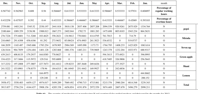
Table (6). The quantity of production (s) at regular time N and overtime O for studied products and their total by the months for 2013
month Jan. Feb. Mar. Apr. May Jun. Jul. Aug. Sep. Oct. Nov. Dec.
Percentage of regular working hours 0.571429 0.571429 0.533333 0.586667 0.56 0.56 0.586667 0.571429 0.586667 0.584615 0.514286 0.593548
O 1135.812 1166.423 1212.061 851.3802 371.16 289.632 1592.836 1978.032 1953.842 480.5849 1773.219 271.2695 Green apple N 0 255.3558 0 387.52 102.0524 0 0 124.4987 214.3627 0 152.2753 197.9538 O 0 191.5169 0 273.0255 80.184 0 0 93.37403 151.0282 0 143.8156 135.5553 Shani N 0 229.8182 244.9455 337.6533 0 0 376.192 266.4727 692.24 121.1004 302.3252 171.6974 O 0 172.3636 214.3273 237.8921 0 0 265.0444 199.8545 487.7145 86.04503 285.5294 117.5754 Lemon N 0 0 0 128.08 0 0 281.696 0 0 0 0 0 O 0 0 0 90.23818 0 0 198.4676 0 0 0 0 0 Total N 4286.94 4464.54 5126.448 4072.896 2513.036 1767.049 6172.123 6993.553 8001.936 4429.748 5351.788 2482.02 O 3215.205 3348.405 4485.642 2869.54 1974.528 1388.396 4348.541 5245.165 5637.728 3147.452 5054.466 1699.644
Table (7). The quantity of production (s) at regular time N and overtime O for studied products and their total by the months for 2014
month Jan. Feb. Mar. Apr. May Jun. Jul. Aug. Sep. Oct. Nov. Dec.
Percentage of regular working hours 0.542857 0.571429 0.586667 0.586667 0.533333 0.586667 0.544 0.541935 0.586667 0.566667 0.551724 0.593548
Table (8). The quantity of production (s) at regular time N and overtime O for studied products and their total by the months for 2015 month Jan. Feb. Mar. Apr. May Jun. Jul. Aug. Sep. Oct. Nov. Dec.
Percentage of regular working hours 0.542857 0.571429 0.613333 0.586667 0.56 0.586667 0.584615 0.567742 0.615385 0.551724 0.586667 0.593548
Percentage of overtime hours 0.457143 0.428571 0.386667 0.413333 0.44 0.413333 0.415385 0.432258 0.384615 0.448276 0.413333 0.406452 product pepsi N 2028.973 2888.847 3436.323 2949.493 2772.417 3169.131 2767.904 4297.048 3801.93 3046.395 1768.24 14528.42 O 1708.609 2166.635 2166.377 2078.052 2178.328 2232.797 1966.669 3271.616 2376.206 2475.196 1245.805 9948.809 Mirnda N 376.4764 304.6026 458.4109 357.632 470.5985 498.08 339.7413 697.2955 537.8517 374.6157 380.4747 1777.1 O 317.0327 228.4519 288.9982 251.968 369.756 350.92 241.3951 530.8954 336.1573 304.3752 268.0617 1216.927 Seven up N 804.761 1334.156 1487.98 1216.597 1491.906 1321.536 1405.235 1542.539 1660.862 1140.8 838.0907 5971.162 O 677.6935 1000.617 938.0744 857.1481 1172.212 931.0822 998.4562 1174.433 1038.038 926.9 590.473 4088.948 Green apple N 320.1919 0 521.0601 230.6187 225.6291 276.56 302.9796 331.9381 316.2573 161.9912 257.8293 1101.971 O 269.6353 0 328.4944 162.4813 177.28 194.8491 215.275 252.7256 197.6608 131.6179 181.6525 754.6107 Shani N 156.6834 314.1506 349.5777 334.352 382.0422 213.4347 436.1656 564.4645 422.1315 254.6006 201.68 1489.127 O 131.9439 235.613 220.3859 235.5662 300.176 150.3744 309.9071 429.7628 263.8322 206.863 142.0927 1019.728 Lemon N 0 0 0 0 0 0 0 0 0 0 0 0 O 0 0 0 0 0 0 0 0 0 0 0 0 Total N 3687.086 4841.756 6253.352 5088.693 5342.593 5478.741 5252.025 7433.285 6739.032 4978.403 3446.315 24867.78 O 3104.914 3631.317 3942.33 3585.216 4197.752 3860.022 3731.702 5659.433 4211.895 4044.952 2428.085 17029.02
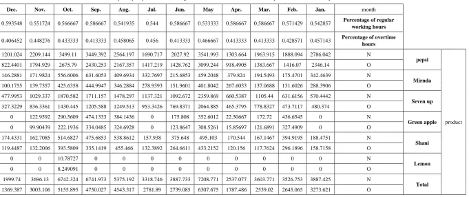
Table (9). The quantity of production (s) at regular time N and overtime O for studied products and their total by the months for 2016
month Jan. Feb. Mar. Apr. May Jun. Jul. Aug. Sep. Oct. Nov. Dec.
Percentage of regular working hours 0.551724 0.57931 0.586667 0.533333 0.586667 0.586667 0.553846 0.593548 0.512 0.551724 0.586667 0.533333
Green apple N 32.66207 332.5452 248.7893 117.9636 255.8507 431.3493 160.8369 347.5604 301.568 221.452 0 307.7624 O 26.53793 241.4912 175.2834 103.2182 180.2584 303.9052 129.5631 238.0033 287.432 179.9298 0 269.2921 Shani N 375.2527 232.2087 295.0187 307.5782 439.4933 582.0427 640.5785 388.3641 275.2279 594.3975 458.48 299.4618 O 304.8928 168.6277 207.8541 269.1309 309.643 410.0755 516.0215 265.945 262.3266 482.948 323.02 262.0291 Lemon N 0 81.46683 171.664 0 174.08 258.784 2792.845 0 112.9984 0 0 0 O 0 59.16044 120.9451 0 122.6473 182.3251 2249.792 0 107.7016 0 0 0 Total N 4359.047 5025.507 5874.736 4147.656 8325.168 6986.24 10050.05 9042.974 6833.529 7533.673 4794.896 3165.619 O 3541.726 3649.475 4139.019 3629.199 5865.459 4922.124 8095.871 6192.471 6513.207 6121.109 3378.222 2769.917
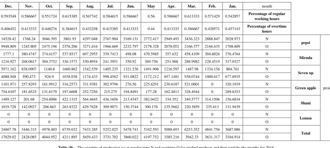
Table (10). The quantity of production (s) at regular time N and overtime O for studied products and their total by the months 2017
month Jan. Feb. Mar. Apr. May Jun. Jul. Aug. Sep. Oct. Nov. Dec.
Percentage of regular working hours 0.606897 0.571429 0.56 0.56 0.586667 0.512 0.586667 0.593548 0.566667 0.593548 0.57931 0.541935
Percentage of overtime hours