MR-DFM: A Multi-path Routing Algorithm Based on
Data Fusion Mechanism in Sensor Networks
Zeyu Sun1,2, Zhiguo Lv1,3
, Yue Hou1, Chen Xu4, and Ben Yan1
1 School of Computer Science and Engineering, Luoyang Institute of Science and Technology,
471023 Luoyang, China
{lylgszy, lzg96wl, houyue0315}@163.com; [email protected]
2 Department of Computer Science and Technology, Xi’an Jiaotong University,
710049 Xi’an, China [email protected]
3 State Key Laboratory of Integrated Services Networks, Xidian University,
710071 Xi’an, China [email protected]
4 School of Computer Science and Information Engineering, Shanghai Institute of Technology
201418, Shanghai, China [email protected]
Abstract. Sensor networks will always suffer from load imbalance, which causes bottlenecks to the communication links. In order to address this problem, a multi-path routing algorithm based on data-fusion-mechanism (MR-DFM) is proposed in this work. In this algorithm, the Mobile Sink controls the clustered energy consumption of the nodes in the event domain according to the delay messages relayed by the neighbor nodes. Meanwhile, the optimal neighbor node in the candidate set is obtained according to the data stream of the neighbor nodes to perform the relay of the data packets. It is shown via simulation results that the proposed MR-DFM algorithm shows obvious improvement according to the energy consumption of the network throughput of the sensing data and the throughput of the sensing data and each hop of the neighbor nodes. Therefore, it is verified that the proposed MR-DFM algorithm shows remarkable data fusion effects and optimizes the network resources.
Keywords: sensor network, data fusion mechanism, multi-path routing, energy consumption, network lifetime.
1.
Introduction
optimization and the data fusion mechanism, the new energy-saving routing technologies have attracted much interest.
The clustering routing protocols divide the WSN into several clusters according to the node energy and the node distance. The nodes within each cluster communicate with the aggregation node through the cluster head. Considering the sharing property of the WSN links, the sensing routing protocol was proposed. In the sensing routing protocol, the transmission strategy of the data packets is controlled by estimating some parameters of the links, such as the signal-to-noise ratio (SNR), delay and load [4-5]. In addition, these parameters are adjusted adaptively according to the network performance. The selecting strategy of the cluster head is modified in paper [6] based on the clustering routing protocols and the remaining energy of the nodes is considered to balance the energy between different nodes and prolong the network lifetime. In paper [7-8], with the rapid development and application of the locating technologies, the geological location based routing protocol has attracted much attention due to its excellent extensibility and adaptability to wireless networks. Based on routing protocol, the core of the geological location is to simply employ the partial topology information which is among different nodes to relay the data in a greedy method to the nearest neighbor node of the destination node. When the data packet reaches a routing void, the flooding, the back-off or the marginal recovery mechanism can be employed to continue the transmission of the data packets. As for the greedy relay mechanism, the expense of any recovery scheme is excessively large. It is an efficient method to saving energy by moving the Sink to a proper site to reduce the data transmission distance. By doing so, the one-hop neighbors of the Sink can be changed so that the hotspot problem can be solved, which no longer becomes the bottleneck of the network performance. The Mobile Sink (MS) [9] can visit every node or only several locations in the network. From the perspective of data routing, the data gathering through the movement of the Sink can be considered as the interception of the data in the routing, i.e., the MS intercepts the transmitted data through some links by proper movement to reduce the network load.
The rest of paper is organized as follows. In Section 2 related work is presented. The data fusion mechanism is given through the network model in Section 3. The multi-route control algorithm is given by the control strategy of the node in Section 4. In Section 5, MR-DFM is assessed by experimental results. Finally, this paper is concluded in Section 6.
2.
Related Work
information entropy of the nodes, the union entropy and the data amount and then obtained High-dimensional Data Aggregation Control (HDAC) in the network through the dynamic scheduling. Nie et.al [11] proposed three different algorithms, i.e., MST-based, DMDC-based and COM algorithms to construct data aggregation trees with better energy consumption performances and delay performances with different data growth rates. The location of the one-hop neighbors or the distance information is employed by the L-PEDAPs [12] to construct the local minimum spanning tree and correlated neighbor graph. Then three different selection methods, i.e. FP, MH and SWP, are adopted for the choosing parent nodes to construct the data aggregation tree. For the WSNs with different initial node energy, Jadidoleslamy Hossein et.at [13] investigated the data aggregation tree problem in the set of shortest path trees which could maximize the network lifetime. This issue is equivalent to finding a shortest path tree with the lightest load. Then it is solved by transforming the shortest to a generalized semi-matcher. A distributed construction algorithm was proposed for the shortest path tree based on depth priority search and width priority search [14, 15]. Wang et.al [16] proposed a dual-tree routing protocol to employ the reverse link and construct two routing trees based on the MST and the DMDC, respectively. For a WSN with multiple mobile Sinks, Zhang et al [17] designed a branch and bound algorithm and an analogous back-fire algorithm to construct the minimum Wiener index spanning tree to obtain better energy efficiency and delay performance for data. It is required in the GSTEB that the Sink designates the root node according to the node energy and the data fusion type while the other nodes choose their father nodes according to their location information and neighbor information. Finally an energy-balanced routing tree is built in a distributed manner.
According to the properties of the routing in WSNs, we perform our study from the following four perspectives Greedy relay strategy based.
(1) The greedy relay strategy could further reduce the energy consumption and reduce the quantity of the hops for the data packets which are from the source node to the sink node.
(2) Predict the routing void. We try to reduce the probability of reaching routing void for the data packets, which could efficiently reduce the routing hops for the data packets.
(3) Avoid the congested links. Nodes in the congested area have to perform many retransmissions to finish transmitting the data packet, which increases the average energy consumption and delay.
(4) Balance the remaining node energy. Excessive use of a certain node would lead to the fast exhaustion of its energy, which further increases the transmission path length for subsequent data packets
3.
Data Fusion Mechanism
3.1. Construction of the Neighbor Nodes
For description convenience, we first give some necessary definitions here. For an arbitrary node i, N(i) is the series of nodes which are neighbor and also can directly communicate with node i and d(i,j) denotes the distance of Euclidean between node i
and node j while R is the wireless transmission radius of the nodes. In the geological routing, the nodes could acquire specific information about neighbor nodes through exchanging the Hello message such as the node ID, geological location, working state and remaining energy. While the node i gets the data packet from the Sink node D, the node i calculates the propelling degree of each neighbor node to the Sink node D as follows:
F(i,j,D)=d(i,D)-d(j,D). (1)
3.2. Neighbors Quantification Based Relay Strategy
While the node i gets a data packet which is p whose destination address is D, a node from N(i) is chosen as the relay node for the next hop according to the relay strategy of the MR-DFM algorithm, which is elaborated as follows.
(1) If node i is exactly the destination of the data packet p, the data packet transmission is successful.
(2) If node j from N(i) is the destination of the data packet p, then that data packet is relayed to node j from node i.
(3) If the destination D lies within the wireless transmission area of node j from
N(i), the data packet p is relayed to node j from node i. If multiple nodes from N(i) satisfies the above condition, F(i,j,D) is calculated according to equation (1) for those nodes. Then the node j with the maximal F(i,j,D) is chosen as the relay node.
(4) If none of the conditions are satisfied, then for an arbitrary node from N(i), the potential propulsion degree from this node to D is calculated according to the corresponding neighbors quantification value.
Ft (i,j,D)=d(i,D)-d(j,D). (2)
Where Ft(j,k,D) is the approximate distance from the nodes in the k-th sector of
node j to D, which can be calculated as follows.
1
2 2 2
2π 2π
Γt j k D, , Γ j k, sin k d j D, Γ j k, cos k
m m
. (3)
Construct the set of candidate relay nodes cs(i). If cs(i) is not empty, then chose
the node j with the maximal Ftn(i,j,D) in cs(i) as the relay node. Otherwise, data
packet p is likely to suffer from routing void at any neighbor of node i. To reduce unnecessary energy consumption, the edge recovery scheme can be employed in advance at node i. cs(i) is expressed as follows:
cs(i)={j|Ftn(i,j,D)>F(i,j,D)}, jN(i). (4)
In comparison with the conventional greedy relay strategy, routing void can be avoided by the nodes utilizing the MR-DFM routing data packet. Therefore, the average energy consumption for data packet transmission can be reduced.
3.3. Data Flow Congestion Avoidance
buffering overflow. Furthermore, employing the retransmission recovery scheme would increase the average energy consumption for transmission.
In order to solve this problem, the greedy relay strategy can be modified by introducing a greediness factor g, which indicates the expected minimal propulsion degree. The factor g is real-valued and ranges from 0 to 1. A small g would increase the path length and the energy consumption for transmission. On the contrary, if g is too large, the number of candidate nodes would decrease and congestion avoidance cannot be achieved. Since the propulsion degree for the candidate node is expected to be at least 80% of the maximal propulsion degree here, we take the value g=0.8. To avoid data flow congestion, we construct the set of candidate relay nodes which satisfies the greediness factor based on the set cs(i).
Gcs(i)={j|Ftn(i,j,D)>gmaxFtn}, jcs(i). (5)
Where maxFtn is the maximal Ftn(i,j,D) in the set cs(i) for node i. A node with the
smallest data flow congestion degree can be chosen as the relay node for the next hop as long as the number of nodes in Gcs(i) is larger than one.
Considering the sharing property of the wireless links between the nodes in the sensor network, the nodes will have more chances to relay data packets when the surrounding links are idle. Otherwise, data packets will be buffered in the node array. The congestion degree of a node within a period of Tcwin is defined as:
cwin(i)=Pin(i)/Ptr(i). (6)
Where Ptr(i) is the number of successfully relayed data packets of node i and Pin(i) is
the average array length for node i within Tcwin.
cwin(i) reflects the node congestion degree within Tcwin. However, during the
transmission of data packets, it is the future congestion degree after the arrival of data packets that we are always concerned about. In order to predict the future congestion degree for the nodes, we employ the exponentially weighted moving average method and define the node congestion degree as:
c(i)=(1-)c(i)+cwin(i). (7) is the weight factor which reflects the real-time varying extent for the node congestion degree. Experiments have shown that when the weight factor takes the value of 0.2, the mean squared error between the predicted value and the realistic value is the smallest. Therefore, we assume =0.2 here.
Considering the fact that the MR-DFM algorithm employs the greedy relay strategy based on two-hop neighbors, the congestion degree of neighbors should also be taken into consideration for the calculation of node congestion degree. The neighbors’ congestion degree is defined as the data flow congestion degree dc(i).
dc(i)=(1-)c(i)+A(j), jN(i). (8)
Where A(j) is the average congestion degree for the neighbor j of node i and is the weight factor for the neighbors.
In order to obtain the data flow congestion degree of the neighbors, dc(i) of node i
can be included in the Hello message. Therefore, we assume Tcwin to be equal to the
3.4. Node Energy Consumption Balance
As is mentioned above, the choice of the relay node for the next hop would influence the network performance to some extent when there are multiple data flows. The reason is that when one node lies on the greedy relay path of multiple data flows, the node energy would be exhausted quickly. If one node is the only greedy relay path for one of the data flows, the failure of this node will cause routing void to this data flow, which will result in sharply increased average energy consumption for this data flow.
For solving this problem, the remained node energy and the number of data flows being relayed have to be taken into consideration to choose the relay node for the next hop. The data flows corresponding to each data packets have to be identified for the counting of data flows. Here, the data flows are distinguished by the source and destination of the data packets. The information on the source node and destination node is extracted from the received data packets by the nodes. If the data flow passes the node for the first time, it will be recorded in the data flow table at the nodes. Otherwise, corresponding records will be updated in the data flow table. Considering the fact that the memory of sensor nodes is limited, only the data flow within the latest period
Tdwinis remained. The number of data flows is:
n(i)=(1-)n(i)+win(i). (9)
Where win(i) is the number of data flows within the latest period Tdwin. Just like the
data flow congestion degree dc(i)of nodes, n(i) is also included in the Hello message.
Furthermore, Tdwin=Tcwin.
n(i) reflects the importance of node i to the transmission of data packet. In order to
avoid the increase of energy consumption for data packet transmission caused by the failure of important nodes, more energy has to be reserved for the nodes with larger n(i), which is referred to as the node energy consumption balance scheme.
The energy balance degree of node i is defined as:
Be(i)=E(i)/n(i). (10)
Where E(i) is the remained energy of node i. A larger E(i) means that node i hopes to relay more data flows or data packets. After the introduction of the node energy balance degree, the relay node weight of each node j in Gcs(i) is calculated as follows
for node i when the relay node for the next hop is chosen based on the greedy relay strategy.
W(j)=Be(j)/dc(j) jGcs(i). (11)
Then the node with the largest W(j) is chosen as the relay node for the next hop. It is shown from the definition of W(j) that node i usually choose the neighbor with smaller congestion degree and higher energy balance degree as the relay for the next hop.
We consider three cases based on the sequential order of the two data flow.
So, when the 10 data packets are relayed for the data flow (B,D), 5 packets are relayed by each one of node C and node F. The first 5 data packets are relayed through node F
while the last 5 packets through node B. The average energy consumption is 2.5, which is normal.
Case 2. The data flow (B,D) comes after flow (A,E). Since there is only one greedy path for flow (A,E), all the 10 data packets are relayed through node F. The energy consumption is 2 on average, which is optimal.
Case 3. When the two flows come simultaneously, at most one data packet of flow (B,D) chooses F as the relay for the next hop. Therefore, n(F)=2while n(C)=1. The
remaining 9 data packets of flow (B,D) choose C as the relay for the next hop, while at most one data packet of flow (A,E) chooses B. The average energy consumption is 2.06, which is near optimal.
Judging from what is analyzed above, the average energy consumption lies between the optimal value and the normal value, regardless of the sequential order of the two flows. The target set for the MR-DFM algorithm is therefore achieved.
4.
Multi-Routing Control Algorithm
4.1. Choice of Cluster Head
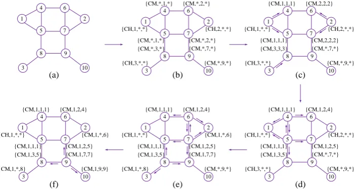
When the event occurs, the nodes in the event domain are distributed into clusters while the cluster heads take charge of the node management and data aggregation. The choices of cluster heads are crucial to the formation of clusters and we can adopt different strategies to maximize the node degree or the remaining node energy, or minimize the identifiers (ID). For the convenience of comparison, we adopt the same choosing strategies for cluster head as in HDAC. The node with the smallest ID in the event domain is chosen as the cluster head. In this stage, the nodes acquire the event monitoring state of neighbors through exchanging the Detecting Message (DM) and further employ the Cluster-Head Announcement (CA) message to contend for the position of cluster head. Both the CA messages and DM are 3-tuples, respectively denoted as <Type, CH_ID, S_ID> and <Type, ID, E_ID>. In the messages, while ID is the node identifier ,Type indicates the message type, E_ID is the identifier of the event,
CH_ID is the identifier of the cluster head and S_ID is the ID of the node which relays
Delay=(TCH-)(X/Xmax). (12)
Where TCH is the duration of the contention sub-period for the cluster head, is the
time required for the CA message to be transmitted all through the event domain which is given empirically, X is the ID of the node with the Role of CH while Xmax is
the largest ID of the nodes.
Through the delayed relay of the CA message, the node which is with the smallest ID will be chosen as the head of the cluster while the corresponding routing structure within the cluster will also be determined. The transmission delay is introduced to guarantee that the cluster head candidate with smaller ID could send the CA message earlier while the amount of CA message sent by cluster head with larger ID can be reduced. Therefore, the control signaling can be efficiently saved.
The choice of cluster head among 10 nodes is illustrated in Fig.1 and the initial distribution of the nodes is shown in Fig.1(a). The nodes first ensure whether they are the cluster head through exchanging the DM message, as shown in Fig.1(b). Next, through a series of relaying of the CA message, node 1 is chosen as the cluster head, which is shown in Fig.1(c)-(f).
4
4 66
5
5 77
1
1 22
8
8 99
3
3 1010
{CH,1,*,*} {CM,*,1,*} {CM,*,1,*} {CM,*,2,*} {CM,*,2,*} {CH,2,*,*} {CM,*,3,*} {CM,*,7,*} {CH,3,*,*} {CM,*,9,*} 4
4 66
5
5 77
1
1 22
8
8 99
3
3 1010
4
4 66
5
5 77
1
1 22
8
8 99
3
3 1010
{CH,1,*,*} {CM,1,1,1} {CM,1,1,1} {CM,2,2,2} {CM,2,2,2} {CH,2,*,*} {CM,3,3,3} {CM,*,7,*} {CH,3,*,*} {CM,*,9,*} 4
4 66
5
5 77
1
1 22
8
8 99
3
3 1010
{CH,1,*,*} {CM,1,1,1} {CM,1,1,1} {CM,1,2,4} {CM,1,2,5} {CH,2,*,*} {CM,1,3,5} {CM,*,7,*} {CH,3,*,*} {CM,*,9,*} 4
4 66
5
5 77
1
1 22
8
8 99
3
3 1010
{CH,1,*,*} {CM,1,1,1} {CM,1,1,1} {CM,1,2,4} {CM,1,2,5} {CM,1,*,6} {CM,1,3,5} {CM,1,7,7} {CM,1,*,8} {CM,*,9,*} 4
4 66
5
5 77
1
1 22
8
8 99
3
3 1010
{CH,1,*,*} {CM,1,1,1} {CM,1,1,1} {CM,1,2,4} {CM,1,2,5} {CM,1,*,6} {CM,1,3,5} {CM,1,7,7} {CM,1,*,8} {CM,1,9,9}
(a) (b) (c)
(f) (e) (d)
Fig. 1. cluster head routing structure
4.2. Communication Correlation among the Nodes
Theorem 1: During the dialogue between terminal a and terminal b, when no node
Proof: If the exposed terminal c is a neighbor of terminal b and terminal a is silent, then according to equation (2), the critical condition for terminal b to correctly receive the data from terminal c is:
Pr(cb)=(+N0)N. (13)
When terminal a and terminal c transmit data simultaneously, the condition for terminal b to correctly receive the data from terminal a is:
Pr(ab)(+Pr(cb)+N0)N. (14)
Substituting equation (13) into equation (14), the condition for terminal b to correctly receive the data from terminal a is:
Pr(ab)/ Pr(cb)N+1. (15)
Similarly, when terminal b and terminal c transmit data simultaneously, the condition for terminal a to correctly receive the data from terminal b is:
Pr(ba)/ Pr(ca)N+1. (16)
Generalizing equation (15), equation (16) and Assumption 2, the condition for transmission of terminal c to pose no influence on Cov(a,b) is:
Pr(ba)/ max(Pr(ca),Pr(cb))N+1. (17)
Similarly, we can derive the condition for transmission of terminal d to pose no influence on Cov(a,b). Therefore, the condition for Cov(c,d) to pose no influence on
Cov(a,b) is:
Pr(ba)/ max(Pr(da),Pr(db),Pr(ca),Pr(cb))N+1. (18)
Finally, we can derive the condition for the case that Cov(a,b) and Cov(c,d) do not influence each other, i.e.,
min(Pr(ba),Pr(cd))/ max(Pr(da),Pr(db),Pr(ca),Pr(cb)) N+1 (19)
The proof is completed.
Corollary 1: When no node synchronization is performed, the condition for the
exposed terminal c to build a new dialogue during the dialogue between terminal a and terminal b is:
f=DX/DMN (20)
Where d is the destination terminal of terminal c, DX=min{d(a,c),d(b,c),d(a,d),
d(b,d)}.
Proof: because DM=max{d(a,b),d(c,d)} and N=(N+1)1/.
1
1 1
a b a c b c
Pr GPt d a,b d a,b d a,b
N N
Pr GPt d c,d d c,d d c,d
.
(21)
min max
'
d a,c ,d b,c ,d a,d ,d b,d DX N DM d a,b ,d c,d
.
(22)
The proof is completed.
4.3. Establishing the algorithm
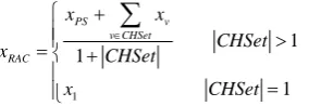
When the cluster is formed based on the event domain or the event is finished, the cluster head has to transmit its location information to the PS through the existing hop tree. According to the information of the cluster heads, the PS calculates the geometric center among the PS and the cluster heads according to equation (21). This center is then chosen as the RAC (Routing Aggregation Center) of the network and further broadcasted all across the network.
1
1
1
1
PS v v CHSet RAC
x x
CHSet
x CHSet
x CHSet
.
(23)
Where CHSet is the set of cluster heads, xRAC、xPS、xvCHSet are the locations of
the RAC, PS and the cluster head, respectively. After the acquisition of the RAC location on the nodes in the network, the nodes is chosen for the next hop which needs the least hops to the PS and closet to the RAC. The algorithms for establishing the MR-DFM routing and updating the routing are explained in details in Table 1 and Table 2, respectively.
Table 1 Algorithm for choosing the cluster head in the MR-DFM
1. FOR each node u which detected the event
2. a DM is sent from u to its neighbors and u waits for a proper time to receive DMs,indent and adjust these things in whole code below. Better use another font for algorithm.;
3. IF ID(v) is bigger than any ID(u)
4. Role(u)=CH; CH_ID1(u)=ID(u); CH_ID2(u)=NULL; 5. ELSE
6. Role(u)=CM; CH_ID1(u)=NULL; CH_ID2(u)=w; 7. IF Role(u)= =CH
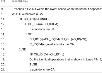
9. u sends a CA out within the event scope when the timeout happens; 10. WHILE u receives a CA
11. IF CH_ID1(u)= =NULL 12. IF CH_ID2(u)<CH_ID(CA) 13. u abandons the CA; 14. ELSE
15. CH_ID1(u)=CH_ID(CA);NH_C(u)=S_ID(CA); 16. S_ID(CA)=u;u retransmits the CA;
17. ELSE
18. IF CH_ID(CA)<CH_ID1(u)
19. Do the identical operations that is shown in Lines 15-18; 20. ELSE
21. u abandons the CA;
Table 2 Algorithm for updating the MR-DFM routing
1. IF an event finishes or occurs
2. The case to the PS was reported by the cluster head of the event; 3. IF CHSet
4. The primary Sink calculates the Routing Aggregation Center (RAC) according to Formula (21), and broadcasts it to the whole network;
5. Each node u finds a neighbor v that satisfies: a)the HTS level is lower than that of u, b) the Euclidean distance to the RAC is the smallest.
6. NH(u)=v;
According to the algorithm for choosing the MR-DFM cluster head, the node is required to make one decision every time it receives one DM message so that it determines whether it should be involved in the contention for the cluster head. The time complexity for this algorithm is O(NN) while the spatial complexity is O(NN)
where NN is the average number of neighbor nodes. Next the nodes involved in the
contention calculate the delay of its CA message and transmits its TA message after the delay. The time complexity of this algorithm is O(1) while its spatial complexity is
complexity for choosing the cluster head in the MR-DFM is O(max(NN, NCH)) while its
spatial complexity is O(NN).
5.
System Evaluation and Simulations
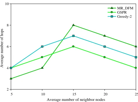
In this paper, we run the simulations to verify the performances of the MR-DFM algorithm on NS-2 (Version NS2.33). We further make comparisons with the conventional greedy routing GSPR algorithm [5] and the two-hop neighbor based Greedy-2 algorithm. The evaluation index is the average hop number, end-to-end delay for transmitting data packets and average energy consumption. I am employed in the simulations while the total number of sensor nodes deployed in each topology is 200. The 802.11 protocol is employed in the MAC layer and the queue length is 50 data packets. The transmission rate of data packets is 11Mb/s and the node socket type is hybrid. The communication radius is 250m. For each type of network topology, 12 different node deployment scenarios are generated uniformly and randomly. The running duration for each simulation is 500s. 10 data streams are randomly chosen among the nodes. The data packet is directly abandoned when it suffers from a routing void. Finally, the results are provided by averaging over the 12 experiments.
Average number of neighbor nodes
A
v
er
ag
e
n
u
m
b
er
o
f
h
o
p
s
5 10 15 20 25
2 4 6 8 10
MR_DFM GSPR Greedy-2
Fig. 2. The average quantity of hops for transmission of the data packet
Running time/s
E
n
er
g
y
c
o
n
su
m
p
ti
o
n
/%
100 200 300 400 500
0 10 20 30 40 50
MR_DFM GSPR Greedy-2
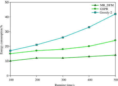
Fig. 3. The average energy consumption for data packet transmission over time
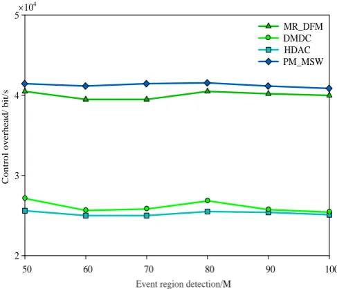
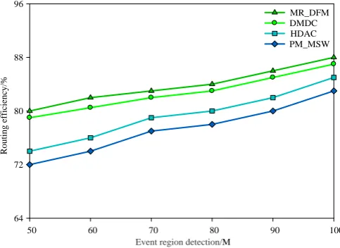
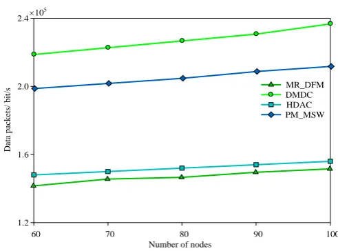
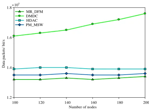
Since the MR-DFM algorithm chooses better nodes for the next hop in the routing updating phase for the sake of data aggregation, the amount of transmitted data in the network for the MR-DFM algorithm is lower than the amount of the HDAC algorithm, which is illustrated in Fig.4. The flooding strategy inside the network is adopted by the HDAC to update the sum of the distance from the nodes to each cluster heads. As a result, far more controlling signaling is required by the HDAC algorithm than the MR-DFM algorithm, the PM_MSW algorithm and the DMDC algorithm. It is won in Fig.5 that with the increasing communication radius, the clustering controlling signaling is increased for the MR-DFM algorithm and the HDAC algorithm, while the MR-DFM algorithm shows a smaller increase. As for the reason, the amount of transmitted CA message can be efficiently reduced by the delay mechanism of the CA message in the MR-DFM algorithm. Since the complete aggregation is adopted, the routing efficiency of all the algorithms increases with the radius of the event domain. Herein, as shown in Fig.6, the MR-DFM algorithm exhibits the highest routing efficiency while the HDAC comes second. It is shown in Fig.7 that the MR-DFM algorithm exhibits the smallest total energy consumption since the MR-DFM algorithm could effectively aggregate data and requires less controlling signaling.
Fig. 4. Performance comparisons with data clustering
Fig. 5. Performance comparisons with controlling signaling
Event region detection/M
C
o
n
tr
o
l
o
v
e
rh
e
a
d
/
b
it
/s
104
MR_DFM DMDC HDAC PM_MSW
50 60 70 80 90 100
2 3 4 5
Event region detection/M
D
a
ta
p
a
c
k
e
ts
/
b
it
/s
105
50 60 70 80 90 100
0.8 1.2 1.6 2.0 2.4 2.8
Fig. 6. Performance comparisons with routing efficiency
Fig. 7. Performance comparisons with total energy consumed
Event region detection/M
R
o
u
ti
n
g
e
ff
ic
ie
n
cy
/%
50 60 70 80 90 100
64 72 80 88 96
MR_DFM DMDC HDAC PM_MSW
Event region detection/M
E
n
er
g
y
c
o
n
su
m
p
ti
o
n
/J
50 60 70 80 90 100
120 150 180 210 240 270
Fig. 8. Performance comparisons with data clustering
Fig. 9. Performance comparisons with controlling signaling
Number of nodes
60 70 80 90 100
C
o
n
tr
o
l
o
v
er
h
ea
d
/
b
it
/s
4 5 6 7 810
4
MR_DFM DMDC HDAC PM_MSW Number of nodes
60 70 80 90 100
D
at
a
p
ac
k
et
s/
b
it
/s
1.2 1.6 2.0 2.4
MR_DFM DMDC HDAC PM_MSW
Fig. 10. Performance comparisons with routing efficiency
Fig. 11. Performance comparisons with total energy consumed
Number of nodes
60 70 80 90 100
E
n
er
g
y
c
o
n
su
m
p
ti
o
n
/J
80 120 160 200
MR_DFM DMDC HDAC PM_MSW
Number of nodes
60 70 80 90 100
R
o
u
ti
n
g
e
ff
ic
ie
n
cy
/%
55 60 65 70
Number of nodes
100 120 140 160 180 200
D
at
a
p
ac
k
et
s/
b
it
/s
1.2 1.4 1.6 1.8
MR_DFM DMDC HDAC PM_MSW
105
Fig. 12. Performance comparisons with data clustering
Number of nodes
100 120 140 160 180 200
C
o
n
tr
o
l
o
v
er
h
ea
d
/
b
it
/s
0 2 4 6 8 10
MR_DFM DMDC HDAC PM_MSW
104
Fig. 14. Performance comparisons with routing efficiency
Fig. 15. Performance comparisons with total energy consumed
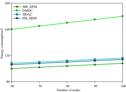
When the area of the network becomes 500m×500m and the radius of the communication becomes 10m, even the number of the nodes changed from 100 to 200, the situation of the algorithm performance is shown in Fig.12- Fig.15. The performance of the algorithm in this paper is higher than other 3 algorithms. With the increase of the node density, the neighbor of the first hop of other 3 kinds of algorithm also increases. Therefore, the average energy consumption of the first hop neighbor in other 3 algorithms are increased. Compared with the 3 algorithms, the energy-efficient result of the algorithm in this paper is higher than 31.26%, 12.26%, 9.68% and 6.31%, respectively. In the aspect of the loss of the data package, the algorithm in this paper is higher than other 3 algorithms as 41.39%, 17.56%, 12.52% and 9.16%, respectively.
Number of nodes
E
n
er
g
y
c
o
n
su
m
p
ti
o
n
/J
MR_DFM DMDC HDAC PM_MSW
100 120 140 160 180 200
100 110 120 130
Number of nodes
100 120 140 160 180 200
R
o
u
ti
n
g
e
ff
ic
ie
n
cy
/%
40 50 60 70 80
In the aspect of the efficiency of routing, the algorithm in this paper is higher than other 3 algorithms as 37.88%, 26.15%, 18.62% and 13.71%, respectively.
6.
Conclusions
A multi-path routing algorithm based on data-fusion-mechanism (MR-DFM) was proposed. After the event occurs, this algorithm could achieve the distributed clustering of the nodes in the event domain with less controlling signaling. After that, the information about the cluster head is sent to the main base station PS by the CH node. The PS calculates the geometric center among itself and all the cluster heads and broadcast the information of center as the routing aggregation center (RAC) across the network. When any node obtains the information of the RAC, it updates the next hop according to its partial state information and finally establishes an approximate Steiner tree. The auxiliary station (AS) moves to the RAC after it receives the information of the RAC and adjusts its location according to the data transmission status of the surrounding neighbors until it can successfully intercept the data. The MR-DFM algorithm could optimize the data aggregation efficiency. Thus, it requires less controlling signaling for the construction and maintenance of the routing. Meanwhile, through the movement of the AS, the information in the network is intercepted to further reduce and balance the data transmission amount in the network as well as alleviate the “hotspot” issue. As a result, an efficient data routing and gathering can be achieved and the network performance is improved. The analyses and simulation results verified the performances of the MR-DFM algorithm.
Acknowledgment. This work is supported by the National Natural Science Foundation of China (No.U1604149); Henan Education Department Young Key Teachers Foundation of China (No.2016GGJS-158); Henan Education Department Natural Science Foundation of China (No.19A520006); High-level Research Start Foundation of Luoyang Institute of Science and Technology(No.2017BZ07); Key Science and Technology Program of Henan Province under Grant 182102210428.
References
1. Meena, U., Sharma, A.: Secure Key Agreement with Rekeying Using FLSO Routing Protocol in Wireless Sensor Network. Wireless Personal Communication, Vol.101, No.2, 1177-1199. (2018)
2. Mohamed, L.M., Hamida, S.: EAHKM+: Energy-aware Secure Clustering Scheme in Wireless Sensor Networks. International Journal of High Performance Computing and Networking, Vol.11, No.2, 145-155. (2018)
3. Zhou, Y. Z., Peng, D. P.: A New Model of Vehicular Ad Hoc Networks Based on Artificial Immune Theory. International Journal of Computational Science and Engineering, Vol.16, No.2, 132-140, (2018)
5. Sasirekha, S., Swamynathan, S.: Cluster-chain Mobile Agent Routing Algorithm for Efficient Data Aggregation in Wireless Sensor Network. Journal of Communication and Networks, Vol.19, No.4, 392-401. (2017)
6. Gao, X. F., Fan, J. H., Wu, F.: Approximation Algorithms for Sweep Coverage Problem with Multiple Mobile Sensors. IEEE/ACM Transactions on Networking, Vol.26, No.2, 990-1003. (2018)
7. Liu, Z. M., Jia, W. J., Wang, G. J.: Area Coverage Estimation Model for Directional Sensor Networks. International Journal of Embedded Systems, Vol.10, No.1, 13-21. (2018) 8. Putra, E. H., Hidayat, R., Widyawan, N.: Energy-efficient Routing Based on Dynamic
Programming for Wireless Multimedia Sensor Networks. International Journal of Electronics and Telecommunications, Vol.63, No.3, 279-283. (2017)
9. Guo, P., Liu, X. F., Cao, J. N.: Lossless In-network Processing and Its Routing Design in Wireless Sensor Networks. IEEE Transactional on Wireless Communications, Vol.16, No.10, 6528-6542. (2017)
10. Sun, Z. Y., Ji, X. H.: HDAC: High-dimensional Data Aggregation Control Algorithm for Big Data in Wireless Sensor Networks. International Journal of Information Technology and Web Engineering, Vol.12, No.4, 72-86. (2017)
11. Nie, Y. L., Wang, H. J, Qin, Y. J.: Distributed and Morphological Operation-based Data Collection Algorithm. International Journal of Distributed Sensor Networks, Vol.13, No.7, 1-15. (2017)
12. Zhao, L. Q., Chen, N.: An improved Zone-based Routing Protocol for Heterogeneous Wireless Sensor Networks. Journal of Information Processing Systems, Vol.13, No.3, 500-517. (2017)
13. Jadidoleslamy, H.: A Hierarchical Multipath Routing Protocol in clustered Wireless Sensor Networks. Wireless Personal Communications, Vol.96, No.3, 4217-4236. (2017)
14. Naidja, M., Bilami, A.: A Dynamic Self-organizing Heterogeneous Routing Protocol for Clustered WSNs. International Journal of Wireless and Mobile Computing, Vol.12, No.2, 131-141. (2017)
15. Das, H. S., Bhattacharjee, S.: A congestion aware routing for lifetime improving in grid-based sensor networks. Journal of High Speed Networks, Vol. 23, No.1, 1-14.(2017) 16. Wang, T., Peng, Z., Liang, J. B.: Follow targets for mobile tracking in wireless sensor
networks. ACM Transactions on Sensor Networks, Vol.12, No.4, 31. (2016)
17. Zhang, Y. Q., Li, Y. R.: A Routing Protocol for Wireless Sensor Networks Using K-means and Dijkstra Algorithm. International Journal of Advanced Media and Communication, Vol.6, No.2-4, 109-121. (2016)
18. Meng, X. L., Shi, X. C, Wang, Z.: A Grid-based Reliable Routing Protocol for Wireless Sensor Networks with Randomly Distributed Clusters. Ad Hoc Networks, No.51, 47-61. (2016)
19. Sun, Z. Y., Zhang, Y. S., Nie, Y. L.: CASMOC: A Novel Complex Alliance Strategy with Multi-objective Optimization of Coverage in Wireless Sensor Networks. Wireless Networks, Vol.23, No.4, 1201-1222. (2017)
20. Wang, T., Peng, Z., Wu, W. Z: Cascading Target Tracking Control in wireless Camera Sensor and Actuator Networks, Asian Journal of Control, 2017,19(4):1350-1364.
21. Ghosh, P., Ren, H., Banirazi, R.: Empirical evaluation of the heat-diffusion collection protocol for wireless sensor networks. Computer Networks, No.127, 217–232. (2016) 22. Wang, S., Yi, H., Wu, L. N.: Mining Probabilistic Representative Gathering Patterns for
Mobile Sensor Data. Journal of Internet Technology, Vol.18, No.2, 321-332. (2017) 23. Chen, Z. S., Shen, H.: A Grid-based Reliable Multi-hop Routing Protocol for
24. Xing, G. L., Li, M. M., Wang, T.: Efficient Rendezvous algorithms for mobility- enabled wireless sensor networks. IEEE Transactions on Mobile Computing, Vol.11, No. 1, 47-60. (2012)
Zeyu Sun received the B.S. degree in computer science and technology from the
Henan University of Science and Technology, in 2003, and the M.Sc. Degree from Lanzhou University, in 2010, and the Ph.D degree form Xian Jiaotong Unviersity, in 2017. He is currently an Associate Professor with the School of Computer and Information Engineering, Luoyang Institute of Science and Technology, Luoyang, Henan, China. His research interests include wireless sensor networks, mobile computing and Internet of Things.
Zhiguo Lv received the B.S. degree in applied electronic technology form Henan
Normal University, in 2000, and the M.Sc. degree in communication and information system from the Guilin University of Electronic Technology, in 2008. He is currently pursuing the Ph.D. degree with Xidian University. He is a Lecturer with the Luoyang Institute of Science and Technology. His research interests include compressive sensing, wireless sensor networks and MIMO system.
Yue Hou is currently pursuing the M.S. degree with Luoyang Institute of Science and
Technology, Her research interests include compressive sensing, wireless sensor networks.
Chen Xu (Corresponding Author) received the M.Sc. degree from Lanzhou Jiaotong
University, in 2010. He is currently pursuing the Ph.D. degree with Tongji University. He is a Lecturer with Shanghai Institute of Technology. His research interests include mobile computing, Intelligent Transportation System and wireless sensor networks.
Ben Yan received the M.Sc. degree in Department of Information Science Okayama
University of Science, Japan, in 2006, and Ph.D. degree in the Graduate School of Information Science at Nara Institute of Science and Technology, Japan, in 2008. His main research interests include the service-oriented architecture, mobile computing and safety critical systems.