Online motion smoothing for video stabilization via constrained multiple-model estimation

(1)

R E S E A R C H

Open Access

Online motion smoothing for video

stabilization via constrained multiple-model

estimation

Chao Jia

1*

and Brian L. Evans

2

Abstract

Video stabilization smooths camera motion estimates in a way that should adapt to different types of intentional motion. Corrective motion (the difference between smoothed and original motions) should be constrained so that black borders do not intrude into the (cropped) stabilized frames. Although offline smoothing can use all of the frames, online (real-time) smoothing can only use a small number of previous frames. In this paper, we propose an online motion smoothing method based on linear estimation applied to a constant-velocity model. We use estimate projection to ensure that the smoothed motion satisfies black-border constraints, which are modeled exactly by linear inequalities for general 2D motion models. We then combine the estimate projection with multiple-model estimation, which can adaptively smooth the camera motion in a probabilistic way. Experimental results show how the proposed algorithm can better smooth the camera motion and stabilize videos in real time.

Keywords: Video stabilization, Kalman filter, Multi-model estimation, Active sets method

1 Introduction

Video data has increased dramatically in recent years due to the prevalence of hand-held cameras. Such videos, however, are usually shakier compared to videos shot by tripod-mounted cameras or cameras with mechanical stabilizers. Digital video stabilization seeks to remove the unwanted frame-to-frame jitter and generate visually stable and pleasant videos. In general, digital video stabilization consists of three major steps, namely motion estimation, motion smoothing, and frame synthesis. This paper focuses on the second step.

Given the estimated camera motion for each frame, motion smoothing aims at designing a new smooth camera motion path. Most existing works address motion smoothing as an offline processing after the entire video sequence has been recorded. However, real-time video stabilization is necessary for applications such as video conferencing and broadcasting. Besides, for consumers who want to record videos, real-time stabilization can greatly improve the user experience with the stabilized

*Correspondence: [email protected] 1_{Qualcomm Inc., 92121 San Diego, CA, USA}

Full list of author information is available at the end of the article

videos displayed in real-time on the viewfinders. Real-time video stabilization is also able to reduce the memory requirements with frames stabilized before compres-sion. In real-time video stabilization, camera motion is required to be smoothed in a causal way. This is more difficult than offline motion smoothing because we are missing information of how camera motion changes afterward.

Due to the camera motion change from motion smooth-ing, some areas in the synthesized frame will be unde-fined. This is known as black-border problem. In practice, we have to crop the resulting video frames and enlarge them if necessary. Still, in motion smoothing, we have to constrain the change of camera motion in order to guarantee that no black borders intrude into the stabilized video frames. How to take such constraint into 5 optimally is a challenging problem, especially for online motion smoothing.

While taking videos, people sometimes move cameras on purpose to get the best viewpoint of the scene that is being recorded. This is known as intentional motion and should be kept by motion smoothing. The changing rate of camera intentional motion may vary, and a fixed motion smoothing strategy may not work well. For instance, aggressive motion smoothing can effectively reduce the

(2)

jitter if the camera motion is supposed to be still, but may lose track of the intentional motion if it is changing fast. Moreover, aggressive motion smoothing for fast changing intentional motion will lead larger areas to be undefined in the stabilized video. As a result, the motion smoothing algorithm should be adaptive accordingly.

In this paper, we propose an online motion smoothing method. Our method is motivated by Kalman-filtering-based motion smoothing with a constant-velocity model. We use Bayesian multiple-model estimation to achieve adaptive smoothing. The black-border constraints are exactly modeled as linear inequalities for almost every 2D motion model. We change the multiple-model estimation algorithm by taking the constraints into account. The state vector estimates are projected onto the constraint set in a probabilistic way.

This paper is organized as follows: Section 2 reviews previous motion smoothing algorithms and related esti-mation background. Section 3 shows how online motion smoothing can be formulated as a linear estimation prob-lem with constant-velocity model that can be solved by Kalman filtering. Section 4.1 formulates the black-border constraints as linear inequalities for most of the 2D camera motion models, and shows how estimate projection can be used to solve the constrained estima-tion problem. Secestima-tion 4.2 presents the proposed adaptive motion smoothing using multiple-model estimation and how to modify it with estimate projection. Section 5 shows how motion smoothing is improved using the pro-posed algorithm of multiple motion models. Section 6 concludes the paper.

2 Background and related work

This paper focuses on motion smoothing. Motion estima-tion, as the other essential step in video stabilizaestima-tion, can be implemented by sparse feature tracking [1] or block matching [2, 3].

Most existing motion smoothing algorithms are offline smoothing. Gaussian window filtering was used to smooth the entire camera motion path in [4, 5] under 2D translational and affine model, respectively. Another kind of algorithms smooth the camera motion via min-imizing a certain objective function that represents the smoothness of the camera motion trajectory. An advan-tage of such objective-minimizing methods is that the black-border constraints can be naturally added to the problem and solved by constrained optimization. In [6], the authors defined the objective function as theL2norm

of the second order difference of camera motion under 2D Euclidean model. The black-border constraint was approximately modeled by an interval constraint on the motion parameters. Similar modeling was also used in [7], but the variables were assumed to be integer-valued and the problem was solved via dynamic programming.

In [8], the objective function was a mixture of the first-, second-, and third order difference of camera motion measured by L1 norm. The motion model was 2D

similarity motion, and the black-border constraint was modeled precisely as linear inequalities. As a result, the constrained motion smoothing could be solved efficiently by linear programming. Black-border constrained was also taken into consideration for window-filtering-based methods. In [9], the authors proposed a dual pass motion smoothing method which could find an optimal cropping size with as large as possible.

In [10], IIR filtering was proposed for online motion smoothing based on 2D translational motion model. Kalman filtering was first used for online smoothing in [11]. The intentional motion parameters (under 2D translational motion model) were modeled by a constant-velocity linear system so Kalman filtering could be used to optimally estimate them. The same Kalman-filtering motion smoothing framework was extended to 2D affine motion model in [12], leading to a better performance. The same algorithm was widely used in the later video stabilization works, such as [1, 13]. These algorithms used fixed parameters in stabilizing the entire video sequence, which is not ideal since the magnitude of unintentional camera motion (jitter) may vary. Adaptive algorithms were proposed for online motion smooth-ing to resolve this problem. In [14], a fuzzy system was used to tune the parameters in an IIR motion fil-ter. A similar fuzzy system was also proposed in [15] to improve the Kalman-filtering-based method. Another adaptive Kalman-filtering method was proposed in [16] by detecting the zero-crossing numbers of motion parame-ters. In our paper, we adaptively estimate the intentional camera motion using dynamic multiple-model estima-tion, which is a generalization of single-mode Kalman filtering [17]. Interacting multiple-model (IMM) algo-rithm [18] has been widely used to solve such prob-lem due to its excellent performance and relatively low computational requirements [19]. Compared to previous adaptive Kalman-filtering-based motion smoothing algo-rithms, the proposed dynamic multiple-model estimation is able to choose the proper parameters optimally from a probabilistic viewpoint. We modified the existing uncon-strained IMM algorithm with estimation projection so that we can successfully smooth the camera motion in an adaptive way while guaranteeing no black borders.

(3)

While [21] still used interval constraints to approxi-mately solve the black-border problem for more com-plicated motion models, in this paper, we use an exact linear inequality modeling of the constraints without any approximation for complicated motion models like simi-larity motion and affine motion. We solve the constrained estimation by estimate projection as proposed in [22]. For a more comprehensive survey of constrained Kalman-filtering algorithms, please see [23].

3 Kalman filter-based motion smoothing

A Kalman filter is an optimal maximum a posteriori (MAP) estimator for linear dynamic systems with Gaus-sian process and measurement noise. Without loss of generality, we assume that there is no control input to the system. The system can be represented as

xk=Fkxk−1+wk

zk =Hkxk+vk , (1)

where xk is the hidden state vector at timek andzk is the observation (or measurement) at time k. Fk is the state transition model which is applied to the previous statexk−1.Hk is the observation model which maps the true state space into the observed space.wk ∼ N(0;Qk) andvk ∼N(0;Rk)model the normal distributed process noise and observation noise. A Kalman filter recursively estimates the Gaussian posterior probabilityp(xk|z1:k)by tracking its mean xˆk and covariance Pk. The Kalman-filtering algorithm can be summarized as Algorithm 1.

Algorithm 1Kalman filtering 1: Input:xˆk−1,Pk−1

2: Output:xˆk,Pk 3: Predict:

4: xˆk|k−1=Fkxˆk−1

5: Pk|k−1=FkPk−1FT_k +Qk 6: Update:

7: yk =zk−Hkxˆk|k−1(innovation)

8: Sk=HkPk|k−1HT_k +Rk (innovation covariance)

9: Kk =Pk|k−1HT_kS−_k1(Kalman gain)

10: xˆk = ˆxk|k−1+Kkyk 11: Pk =(I−KkHk)Pk|k−1

12: end

Kalman filtering with a constant-velocity (CV) system model has been widely used in tracking maneuvering tar-gets. Assuming one dimension of the target location to be tracked isxk, the CV model uses a state vectorxk =

[xk,vk]T consisting of both xk and the velocity in this dimensionvk. The dynamic model is specified as

Fk=

1 T

0 1 ,

wk∼N

0;σ_p2 T4 4 T 3 2 T3

2 T2

, (2)

whereTis the sampling interval. In this model, the veloc-ity is assumed to be almost constant except for a possible acceleration (maneuvering) with distribution N(0;σ_p2). Usually, we have a noisy measurement of the location of the target, so the measurement model can be specified as

Hk = 1 0

,vk∼N

0;σ_m2. (3)

The aforementioned single-dimensional CV model can be easily generalized to a multi-dimensional CV model. The Kalman filter estimate of the target locations from the CV model usually appears much smoother com-pared to the original noisy location measurements due to the constant-velocity assumption in the dynamic model. Therefore, this model has been successfully used in causal smoothing of time series such as the camera motion.

Given a reference frame, the camera motion of the entire video sequence can be represented as a sequence of motion parameters dependent on the choice of motion model. For instance, a 2D affine model depicts the relative transformation between two frames as

x y =A x y

+b, (4)

where [x,y]Tand [x,y]T are the locations of any pair of matched pixels in the two frames. Therefore, the camera motion of each framek can be represented by a 2 ×2 matrixAk and a 2×1 vectorbk. In general, the camera motion of the video can be parameterized as a sequence of motion vectors{θ_k}. This sequence can then be smoothed via the CV-model-based Kalman filtering by setting the state vector as [θk,θ˙k]T, whereθ˙kis the discrete changing rate (velocity) of the camera motion.

4 The proposed methods

(4)

4.1 Constraints on motion smoothing and constrained Kalman filtering

The smoothed camera motion generates a correction motion for each frame. In the last step of video stabiliza-tion, the new frames are synthesized by image warping using the correction motion. The synthesized frames may contain black borders since not every pixel in the syn-thesized frame is visible in the original frame due to the change of camera motion. As discussed in Section 2, a secure way to this problem is to crop the synthesized frames into a smaller size so that there are no black bor-ders in the stabilized video. Therefore, in smoothing the camera motion sequence, we need to guarantee that every pixel in the cropped stabilized frames is visible in the original frames. This is a hard constraint that has to be considered in the camera motion smoothing algorithm.

For almost all kinds of 2D motion models, the con-straints on the camera motion parameters for each frame can be expressed as a set of linear inequality constraints. Thus, the system we are facing becomes

xk =Fkxk−1+wk

zk=Hkxk+vk s.t.kxk≤βk. (5)

The state constraints have to be taken into account in Kalman filtering. We tackle this problem with an effi-cient method known as estimate projection. The idea is to project the unconstrained state estimatexˆkof the Kalman filter onto the constraint set. The constrained estimate can be written as

˜

xk =argminx(x− ˆxk)TW(x− ˆxk), s.t.kx≤βk, (6)

whereWis a positive-definite weighting matrix. Usually, W is chosen as the inverse of the unconstrained covari-ance matrix estimate P−_k1. In this way, the solution x˜k maximizes the probability density function (pdf ) of the original unconstrained estimate subject to the state con-straints. Note that (6) is a linear-inequality-constrained convex quadratic programming (QP) problem. We solve it using the active set method. The active set method searches the constraints that are active at the optimal solution to the problem. For each trial of active con-straints, the problem is simplified to a linear-equality-constrained quadratic programming problem, which can be solved analytically in one step using Lagrange mul-tiplier method. Details of active set method for convex QP are shown in [24].

In the next subsections, we show the modeling of the visibility constraint as a set of linear inequality constraints for three different camera motion models:

4.1.1 Affine motion

Under affine motion, a pixel [x,y]T in frame k can be transformed to location

x y =

a0_k a1_k a2_k a3_k

x y

+

b0_k b1_k

(7)

in the reference frame using six parameters. We assume that the smoothed camera motion for framekisaˆi

k,i = 0· · ·3 andbˆi_k,i=0, 1. Then, given the four corners of the cropping rectangle [ci_x,ci_y]T,i=1· · ·4, the constraints on the smoothed camera motion can be represented as

0 0 ≤

a0_k a1_k a2_k a3_k

−1

ˆ

a0_k aˆ1_k

ˆ

a2_k aˆ3_k ci_x ci_y

+

ˆ

b0_k

ˆ

b1_k

−

a0_k a1_k a2_k a3_k

−1 b0_k b1_k ≤ w h , (8)

where wandh are the width and height of the original frame. This is a set of linear inequality constraints on the smoothed motion parameters.

4.1.2 Similarity motion

The similarity motion model is similar to the affine motion model except thata2_kis forced to be equivalent to −a1_k , anda3_kis forced to be equivalent toa0_k. So, there are four motion parameters for each frame instead of six in the affine motion model.

4.1.3 Translation motion

The translation model only depicts the 2D translation motion of pixels on the image plane, so it forces the matrix

a0_k a1_k a2_k a3_k

to be identified and only leaves translational

parametersb0_kandb1_k.

The constraints on the smoothed camera motion can be represented as

0≤ci_x+ ˆb0_k−b0_k≤w

0≤ci_y+ ˆb_k1−b1_k ≤h, (9)

which can be further simplified to an interval constraint.

4.2 Adaptive smoothing with multiple-model estimate

4.2.1 Adaptive motion smoothing

Motion smoothing using CV model highly depends on the assumption of the acceleration variance (σpin (2)). Small value ofσpallows little change in velocity, which results in a smoother trajectory. On the opposite, large value of σpgives higher degree of flexibility in velocity change and leads to a trajectory closer to the original one (given as the noisy measurement).

(5)

motion. Moreover, the smoothed camera motion gener-ated by Kalman filtering with smallerσptends to deviate farther from the original camera motion, and thus trig-gers estimate projection in Section 4.1 more frequently. As shown in Section 4.1, the constraints on motion parametersθˆkare determined by the original (unsmooth) motion parameters θk, and therefore differ across dif-ferent frames. Frequent estimate projection may add the unwanted camera shake back and reduce the smoothness of the Kalman-filtering output.

Therefore, it is desirable to adaptively change the value of σp according to the original camera motion. For the frames which the intentional camera motion is still, we would better use small value of σp to effectively elimi-nate camera shake (measurement noise in (1)). For the frames which the intentional camera motion changes fast, a larger value ofσpcan provide the flexibility in tracking the camera motion change and avoid estimate projection for satisfying the black-border constraint.

We solve this problem via dynamic multi-model state estimate. We useMdifferent CV system models{j,j =

1· · ·M}that only differ in the value ofσp. The model is assumed to jump between models as a Markov chain:

p(m_k₊₁=j|m_k =i)=pij. (10)

If the model is static, we can implementMKalman fil-ters in parallel with each corresponding to a model. At each stage, likelihood of each modelp(mk|z1:k) is com-puted first and the state estimate is comcom-puted as a Bayes-optimal combination of the the individual estimates. If the model is dynamic as in our case, the optimal multi-model filter has to keep track of all of the model history, which grows exponentially with increasing stages (frames). In practice, only model history in the last stage is kept and the model histories in older stages are combined. This idea leads to the IMM (interacting multiple-model) algo-rithm, which has good performance and relatively low computational complexity.

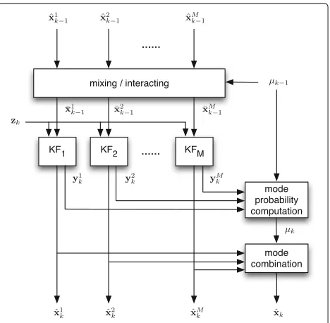
4.2.2 IMM algorithm

An unconstrained IMM estimator consists of three main steps: (1) mixing/interacting of the mode-conditioned estimates in previous stage, (2) mode-conditioned state estimation, and (3) mode probability computation. Figure 1 illustrates how IMM algorithm is implemented. At each stage, we keep the Gaussian approximations of each mode-conditioned estimatep(xk|mk = j,z1:k)with meanxˆj_kand covariancePj_k. The mode probabilitiesμj_k=

p(m_k =j|z1:k)are also kept.

In the mixing step, we obtain p(xk−1|mk = j,z1:k−1)

according to

M

i=1

p(xk−1|mk−1=i,z1:k−1)λij_k₋₁, (11)

Fig. 1Unconstrained IMM algorithm

whereλij_k₋₁ = p(mk−1 = i|mk = j,z1:k−1).λij_k₋₁can be

computed by Bayes rule using the mode transition proba-bility and the mode distribution in the previous stageμk−1

as

λij k−1=

p(mk−1=i,mk =j|z1:k−1)

M

i=1p(mk−1=i,mk =j|z1:k−1)

= μ

i k−1pij

M

i=1μik−1pij

. (12)

Note that (11) is a mixture of Gaussian distribution. The IMM algorithm approximates it by a Gaussian distribu-tion with meanx¯j_k₋₁and covarianceP¯j_k₋₁.

Each pair of x¯j_k₋₁,P¯j_k₋₁ is then fed into a Kalman fil-ter to getp(xk|mk = j,z1:k)(represented by meanxˆj_kand covariancePˆj_k).

The mode probabilities are updated according to

μj

k ∝p(mk =j,zk|z1:k−1)

=p(mk=j|z1:k−1)p(zk|mk=j,z1:k−1)

=

_M

i=1 μi

k−1pij

p(zk|mk =j,z1:k−1), (13)

wherep(zk|mk = j,z1:k−1)is equivalent to the

probabil-ity of the innovation vectoryj_k with respect to a Gaussian distributionN(0;Sj_k)(see line 8 and 9 in Algorithm 1).

(6)

4.2.3 Constrained IMM algorithm

In this subsection, the black-border constraints in Section 4.1 is applied to the multi-model estimation. We have shown that the constraints can be modeled as a set of linear inequality constraints. In single-model Kalman filtering, error projection method can be applied on the unconstrained Kalman filter estimate to meet the con-straints. The output of the IMM algorithm consists of the outputs of several Kalman filters, as well as their combina-tion using the mode probabilities. Therefore, we can also apply error projection (6) on the unconstrained estimate of each Kalman filter. Their linear combination automat-ically satisfies the constraints due to the linearity of the constraints.

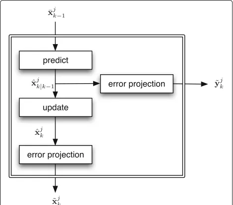
Such modification can guarantee the constraints being satisfied. However, the influence of the constraints on the computation of mode probabilities is not taken into account. Error projection was proposed after both predict and update steps have been implemented. Therefore, the innovation vectors are not modified and the mode proba-bility computation remains unchanged. To make the mode probabilities to better reflect the influence of the black-border constraints, we propose to insert an additional error projection step between the predict and update steps in each Kalman filters in the IMM algorithm. The input (innovation vectors) to mode probability computa-tion step is a modified version after error projeccomputa-tion. Note, however, the update step in each Kalman filter still use the unchanged predicted state vector because there will be another error projection step after update.

The modified Kalman filter for constrained IMM algorithm is illustrated by Fig. 2 and summarized in Algorithm 2.

Fig. 2Modified Kalman filter in constrained IMM algorithm

Algorithm 2Modified Kalman filter in constrained IMM algorithm (same for anyj=1· · ·M)

1: Input:x¯j_k₋₁,Pj_k₋₁

2: Output:x˜j_k,P_kj,y˜j_k,Sj_k 3: Predict:

4: xˆj_k_|_k₋₁=Fkx¯j_k₋₁

5: Pj_k_|_k₋₁=Fj_kPj_k₋₁Fj_kT+Qj_k 6: 1st Error projection:

7: x˜j_k_|_k₋₁=argmin_x(x−ˆxj_k_|_k₋₁)TPj_k_|_k₋₁−1(x−ˆxj_k_|_k₋₁), s.t.kx≤βk

8: y˜j_k =zk−Hjkx˜ j

k|k−1(modified innovation)

9: Update:

10: yj_k =zk−H_kjxˆj_k_|_k₋₁(innovation)

11: Sj_k =Hj_kPj_k_|_k₋₁Hj_kT+Rj_k(innovation covariance)

12: Kj_k=Pj_k_|_k₋₁Hj_kTSj_k−1(Kalman gain)

13: xˆj_k= ˆxj_k_|_k₋₁+Kj_kyj_k

14: Pj_k=

I−Kj_kHj_kPj_k_|_k₋₁

15: 2nd Error projection:

16: x˜j_k=argmin_x(x− ˆxj_k)TPj_k−1(x− ˆxj_k), s.t.kx≤βk

17: end

5 Experimental results and discussion

5.1 2D translational motion

We first test the proposed algorithm under a 2D trans-lational motion model. As we see in Section 4.1.3, the black-border constraints can be modeled as independent interval constraints on the two parameters of camera motion (displacements in x and y axes). As a result, the two motion parameters can be smoothed separately, which makes visual and numerical comparison of different algorithms easier.

5.1.1 Synthetic motion

Figure 3 shows a synthetic path of image displacement for a video with 600 frames and the smoothed result using the proposed algorithm. The intentional motion has con-stant velocity except for the abrupt changes at frames 200 and 400. The unsteady (original) motion is synthesized by adding Gaussian random noise to the intentional motion. We constrain the motion smoothing so that the correc-tion translacorrec-tion on each direccorrec-tion is less than 60 pixels. In the multiple-model estimation, we use two modes with σ2

pT2 = 0.0001 andσp2T2 = 0.1 (pixels2). The sampling intervalT is 33.3 ms, which corresponds to 30 fps. The mode transition probability is set as p11 = 0.99,p12 =

0.01,p21 = 0.25, andp22 = 0.75. Such setting has a bias

(7)

0 100 200 300 400 500 600 0

100 200 300 400 500 600 700 800

Frame

Image displacement (pixels)

Original Smoothed

Fig. 3Synthetic simulation: original and smoothed motion using the proposed approach

0 100 200 300 400 500 600

−100 0 100 200 300 400 500 600 700 800

Frame

Image displacement (pixels) _{Constrained KF with small}_σ

p

Constrained KF with large σ_p

Constrained IMM

Fig. 4Synthetic simulation: comparison between single-model constrained Kalman filtering and constrained IMM.Cyan curvesare constraint boundaries

0 100 200 300 400 500 600

0 0.1 0.2 0.3 0.4 0.5 0.6 0.7 0.8 0.9 1

Frame

Probability

Probability of mode with large σ_p Probability of mode with small σ_p

(8)

Table 1Numerical comparison between different motion smoothing algorithms for the synthetic camera motion

Mean square jitter Mean square acceleration

Unsmoothed 314.00 2217.43

Smallσp 11.58 21.79

Largeσp 19.24 28.09

Proposed 3.93 10.80

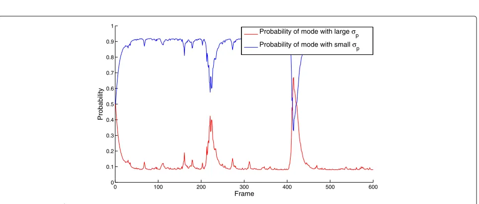
In Fig. 4, we compare the proposed constrained IMM with single-model constrained Kalman filters. We also show the constraint boundaries by cyan curves. We can find that the result of constrained IMM is closer to the result of Kalman filter with largeσpbut clearly smoother (better observed after zooming in). The result of Kalman filter with small σpappears smoother when the velocity of the intentional motion does not change, as expected. However, when there is an abrupt change in the velocity, it takes longer to adapt to the correct velocity estima-tion. This leads to more jitters after frame 200 and frame 400 because the Kalman filter estimates before estimation projection hits the constraint boundaries more often.

Figure 5 shows how the mode probabilities change in the multiple-model estimation. Sudden changes of pixel displacement velocity clearly corresponds to the increase in probability of mode σ2

pT2 = 0.1 and decrease in probability of modeσ_p2T2=0.0001.

In numerical comparison, we use two performance met-rics. The first is the mean square of jitter in the result. The jitter is obtained by passing the result through a high pass filter with cutoff frequency as 1 Hz (sampling fre-quency is 30 Hz). This metric was proposed in [25]. In [25], another metric was proposed with the mean square of jitter to measure the low-frequency divergence between the smoothed motion and the intentional motion. In this paper, the black-border constraints naturally restrict such divergence to a very small value. So, we only use the mean square of jitter because it reflects the smoothness of the camera motion.

The other smoothness metric we measure is the mean square of the motion acceleration. Motion acceleration is the second order difference of the motion parame-ter sequence. This metric is widely used as the objective function to minimize many offline video stabilization algorithms [6, 8].

Table 1 shows the numerical comparison between single-model constrained Kalman filtering and con-strained IMM. From Table 1, we can see that for both smoothness metrics, the constrained IMM outperforms the single-mode constrained Kalman filters.

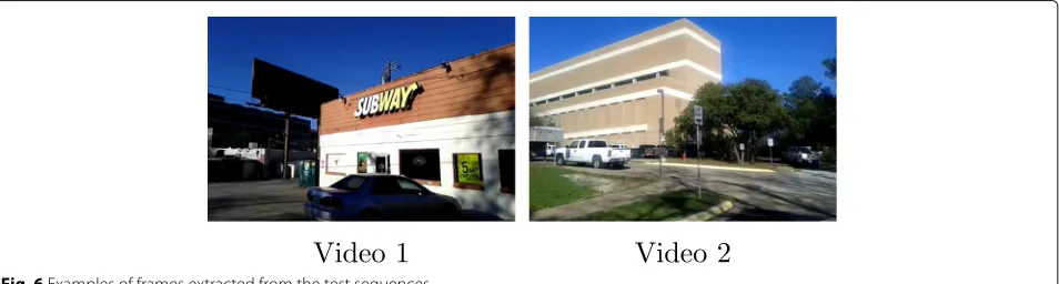
5.1.2 Real videos

We also tested the proposed algorithm on two real videos. Both videos are captured by a walking person on urban streets. Figure 6 shows two example frames extracted from the videos. The original frame size is 720×480. In our experiments, we use a 540× 360 cropping size for the stabilized video. The choice ofσpand mode transition matrix are the same as in the synthetic simulation.

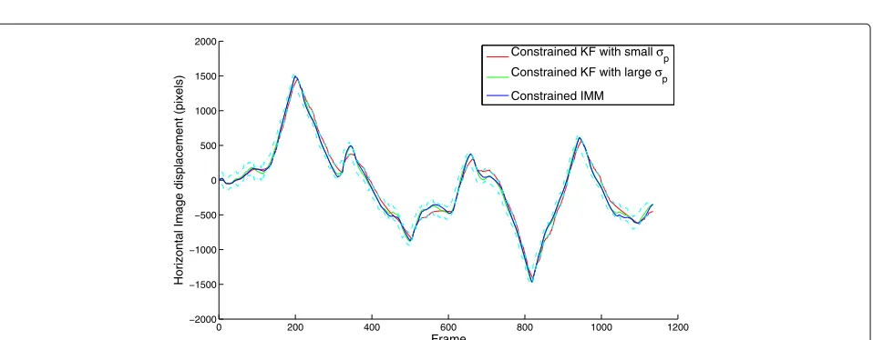
Figures 7 and 8 show the smoothed horizontal motion of video 1 and video 2 using single-model constrained Kalman filters and the proposed constrained IMM fil-ter. Similar to the synthetic simulation, the proposed IMM filter performs well no matter the velocity of the intentional motion stays almost constant or changes abruptly.

The smoothed vertical motions of two test videos are shown in Figs. 9 and 10, respectively. Vertical translations of videos are more unstable because the photographer is walking. Also, the intentional motion of vertical trans-lation does not have very large changes in its velocity because the urban street is even. Therefore, constrained Kalman filter with smaller σp seems to perform better, especially for video 2.

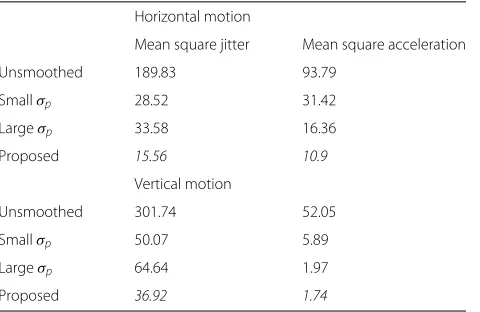
Numerical comparisons in Tables 2 and 3 show that the proposed algorithm can smooth the entire video sequences better except for the vertical motion of video 2.

(9)

0 100 200 300 400 500 600 700 800 900 1000 −1000

−500 0 500 1000 1500 2000

Frame

Horizontal Image displacement (pixels)

Constrained KF with small σ_p Constrained KF with large σ_p Constrained IMM

Fig. 7Video 1 horizontal motion: comparison between single-model constrained Kalman filtering and constrained IMM.Cyan curvesare constraint boundaries

0 200 400 600 800 1000 1200

−2000 −1500 −1000 −500 0 500 1000 1500 2000

Frame

Horizontal Image displacement (pixels)

Constrained KF with small σ_p Constrained KF with large σ_p Constrained IMM

Fig. 8Video 2 horizontal motion: comparison between single-model constrained Kalman filtering and constrained IMM.Cyan curvesare constraint boundaries

0 100 200 300 400 500 600 700 800 900 1000 −100

0 100 200 300 400 500

Frame

Vertical Image displacement (pixels)

Constrained KF with small σ_p

Constrained KF with large σ

p

Constrained IMM

(10)

0 200 400 600 800 1000 1200 −200

−100 0 100 200 300 400

Frame

Vertical Image displacement (pixels)

Constrained KF with small σ_p

Constrained KF with large σ

p

Constrained IMM

Fig. 10Video 2 vertical motion: comparison between single-model constrained Kalman filtering and constrained IMM.Cyan curvesare constraint boundaries

5.2 2D affine motion

2D affine motion can model the pixel displacements more accurately than 2D translational motion. There-fore, motion smoothing under 2D affine motion model can generate more stable videos than 2D translational motion. For 2D affine motion model, the black-border constraints can be exactly modeled by linear inequali-ties as in (8). Such constraints can be efficiently han-dled by the proposed estimation projection steps in the IMM estimation framework. Multiple-model filtering is only used to smooth motion parameters b0 and b1 to reduce the necessary number of modes. The parameters

a0· · ·a3 are still smoothed by single-mode Kalman fil-tering. Similar to 2D translational motion smoothing, we use two modes (σ2

pT2 = 0.0001 and σp2T2 = 0.1) for each ofb0andb1. Since for 2D affine motion model the

motion parameters cannot be smoothed independently,

Table 2Numerical comparison between different motion smoothing algorithms for video 1

Horizontal motion

Small_σp 28.52 31.42

Largeσp 33.58 16.36

Proposed 15.56 10.9

Vertical motion

Smallσp 50.07 5.89

Largeσp 64.64 1.97

Proposed 36.92 1.74

we have four modes in total in the constrained IMM filtering.

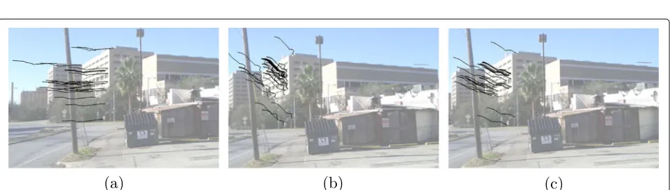
We compare the motion smoothing results visually by showing the feature trajectories in the stabilized videos. Specifically, we detect Harris corner points in a cer-tain frame and track them for 20 frames. The feature trajectories are plotted as black curves on top of the starting frame (the frames themselves are plotted using alpha channel 0.5 (more transparent) to make the curves clearer). For a stabilized video, the trajectories should look smooth. Figure 11 shows a comparison between the stabilization results using the proposed 2D trans-lational motion smoothing and the proposed 2D affine motion smoothing. Note that we detect and track the feature points independently in the three videos so the location and number of the feature points can be differ-ent. It is clear that affine motion smoothing can better

Table 3Numerical comparison between different motion smoothing algorithms for video 2

Horizontal motion

Small_σp 122.86 32.44

Largeσp 113.54 15.77

Proposed 93.59 11.47

Vertical motion

Smallσp 1.43 0.61

Largeσp 44.17 1.35

(11)

Fig. 11Stabilization comparison for video1. Features are tracked from frame 256 to frame 275. The feature tracks are plotted asblack curveson frame 256.aOriginal video.bProposed translational smoothing.cProposed affine smoothing

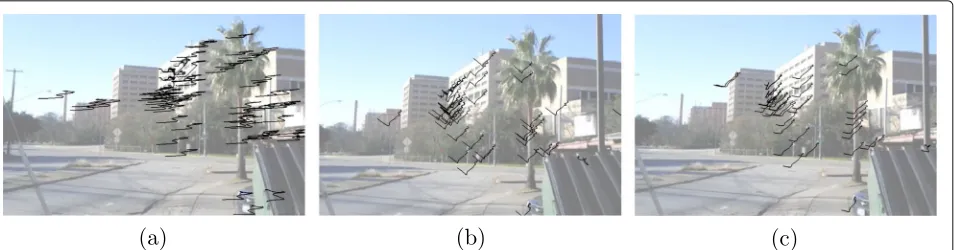
Fig. 12Stabilization comparison for video 2. Features are tracked from frame 16 to frame 35. The feature tracks are plotted asblack curveson frame 16.aOriginal video.bProposed translational smoothing.cProposed affine smoothing

(12)

Fig. 14Stabilization comparison for video 1. Features are tracked from frame 700 to frame 719. The feature tracks are plotted asblack curveson frame 700.aConstrained KF with small_σp.bConstrained KF with largeσp.cConstrained IMM filter

stabilize the original video under the same black-border constraints. Figure 12 shows a similar comparison for video 2. As a result, it is necessary to stabilize the videos using affine motion model if we want to get more stable results.

We next compare the stabilized results using the constrained IMM filter against single-mode constrained Kalman filters, all using 2D affine motion model. As shown in Figs. 13 and 14, in the cases where the velocity of the intentional camera motion changes slowly, con-strained Kalman filter with small σp tends to generate the most stable results. However, when there is abrupt velocity change in the intentional motion, the constrained Kalman filter with smallσp can result in annoying back and forth pixel movements because the motion esti-mate hits the constraints easily. The proposed constrained multiple-model filter is able to generate more balanced results, which is consistent with our observation and anal-ysis in Section 5.1.

6 Conclusions

In this paper, we propose an online motion smoothing method for video stabilization based on the existing constant-velocity Kalman-filtering method. The black-border constraints are modeled as linear inequalities for different 2D motion models and are combined with the Kalman-filtering framework in a probabilistic way. Estimate projection is used to project the estimates on to the constraint set after the update step in Kalman filtering. To adaptively smooth the camera motion with different kinds of intentional motion, we propose to use multiple-model estimation with different process noise variance instead of single-mode Kalman filtering. To make the mode probability computation more accurate under the affect of black-border constraints, the multiple-model estimation is modified by adding another estimate projection step after the propagation step for each sub-filter. Experimental results show that the proposed constrained multiple-model estimation is able to

adaptively smooth camera motion and guarantee that all of the pixels in stabilized frames are defined in the original frames.

Funding

This research was supported by a gift funding from Texas Instruments, Dallas, TX, USA.

Authors’ contributions

CJ designed the proposed algorithm, carried out the experiments, and drafted the manuscript. BE participated in the discussion of algorithm design and modified the content of the manuscript. Both authors read and approved the final manuscript.

Competing interests

The authors declare that they have no competing interests.

Author details

1_{Qualcomm Inc., 92121 San Diego, CA, USA.}2_{Department of Electrical and} Computer Engineering, The University of Texas at Austin, 78712 Austin, TX, USA.

Received: 27 September 2016 Accepted: 16 February 2017

References

1. J Yang, D Schonfeld, M Mohamed, Robust video stabilization based on particle filter tracking of projected camera motion. IEEE Trans. Circ. Syst. Video Technol.19(7), 945–54 (2009)

2. C Yan, Y Zhang, J Xu, F Dai, J Zhang, Q Dai, F Wu, Efficient parallel framework for HEVC motion estimation on many-core processors. IEEE Trans. Circ. Syst. Video Technol.24(12), 2077–89 (2014)

3. C Yan, Y Zhang, J Xu, F Dai, L Li, Q Dai, F Wu, A highly parallel framework for HEVC coding unit partitioning tree decision on many-core processors. IEEE Signal Process. Lett.21(5), 573–6 (2014)

4. S Ertürk, TJ Dennis, Image sequence stabilization based on DFT filtering. IEE Proc. Vision Image Signal Process.147(2), 95–102 (2000)

5. Y Matsushita, E Ofek, W Ge, X Tang, H-Y Shum, Full-frame video stabilization with motion inpainting. IEEE Trans. Pattern Anal. Mach. Intell. 28, 1150–1163 (2006)

6. C Song, H Zhao, W Jing, Y Bi, inProc. Intl. Conf. Pattern Recognition. Robust video stabilization based on bounded path planning, (2012)

7. M Pilu, inProc. IEEE Intl. Conf. Computer Vision and Pattern Recognition. Video stabilization as a variational problem and numerical solution with the viterbi method, (2004)

8. M Grundmann, V Kwatra, I Essa, inProc. IEEE Conf. Computer Vision and Pattern Recognition. Auto-directed video stabilization with robust l1 optimal camera paths, (2011)

(13)

10. S Ertürk, inProc. Intl. Symp. Image and Signal Processing and Analysis. Image sequence stabilization: motion vector integration (MVI) versus frame position smoothing (FPS), (2001)

11. S Ertürk, Real-time digital image stabilization using Kalman filters. Real-Time Imaging.8, 317–28 (2002)

12. A Litvin, J Konrad, W Karl, Probabilistic video stabilization using Kalman filtering and mosaicking. Proc. IS&T/SPIE Symp. Electronic Imaging, Image and Video Comm. and Proc.5022, 663–74 (2003)

13. C Jia, Z Sinno, B Evans, inProc. Asilomar Conf. Signals, Sytems, and Computers. Real-time 3D rotation smoothing for video stabilization, (2014) 14. MJ Tanakian, M Rezaei, F Mohanna, Digital video stabilizer by adaptive

fuzzy filtering. EURASIP J. Image Video Process.21(2012) 15. Güllü, E Yaman, S Ertürk, Image sequence stabilization using fuzzy

adaptive Kalman filtering. Electron. Lett.39, 429–31 (2003)

16. C Wang, J-H Kim, K-Y Byun, J Ni, S-J Ko, Robust digital image stabilization using the Kalman filter. IEEE Trans. Consum. Electron.55(1), 6–14 (2009) 17. Y Bar-Shalom, XR Li, T Kirubarajan,Estimation with applications to tracking

and navigation: theory algorithms and software. (J. Wiley and Sons, 2001) 18. HAP Blom, Y Bar-Shalom, The interacting multiple model algorithm for

systems with Markovian switching coefficients. IEEE Trans. Autom. Control.33(8), 780–3 (1988)

19. E Mazor, A Averbuch, Y Bar-Shalom, J Dayan, Interacting multiple model methods in target tracking: a survey. IEEE Trans. Aerosp. Electron. Syst.34, 103–23 (1998)

20. M Tico, M Vehvilainen, inProc. IEEE Intl. Conf. Image Processing. Constraint motion filtering for video stabilization, (2005)

21. M Tico, M Vehvilainen, inProc. European Signal Processing Conference. Constraint translational and rotational motion filtering for video stabilization, (2005)

22. D Simon, DL Simon, Aircraft turbofan engine health estimation using constrained Kalman filtering. ASME J. Eng. Gas Turbines Power.127, 323–8 (2005)

23. D Simon, Kalman filtering with state constraints: a survey of linear and nonlinear algorithms. IET Control Theory Appl.4, 1303–18 (2010) 24. J Nocedal, SJ Wright,Numerical optimization. (Springer, 1999) 25. M Niskanen, O Silven, M Tico, inProc. IEEE Intl. Conf. Multimedia and Expo.

Video stabilization performance assessment, (2006)