www.mech-sci.net/4/139/2013/ doi:10.5194/ms-4-139-2013
©Author(s) 2013. CC Attribution 3.0 License.
Mechanical
Sciences
Open Access
A new variable stiffness suspension system:
passive case
O. M. Anubi, D. R. Patel, and C. D. Crane III
Center for Intelligent Machines and Robotics, Department of Mechanical and Aerospace Engineering, University of Florida, Gainesville, Florida, USA
Correspondence to: O. M. Anubi ([email protected])
Received: 15 November 2012 – Accepted: 15 January 2013 – Published: 26 February 2013
Abstract. This paper presents the design, analysis, and experimental validation of the passive case of a vari-able stiffness suspension system. The central concept is based on a recently designed variable stiffness mech-anism. It consists of a horizontal control strut and a vertical strut. The main idea is to vary the load transfer ratio by moving the location of the point of attachment of the vertical strut to the car body. This movement is controlled passively using the horizontal strut. The system is analyzed using anL2-gain analysis based on the concept of energy dissipation. The analyses, simulation, and experimental results show that the variable stiff -ness suspension achieves better performance than the constant stiffness counterpart. The performance criteria used are; ride comfort, characterized by the car body acceleration, suspension deflection, and road holding, characterized by tire deflection.
1 Introduction
Improvements over passive suspension designs is an active area of research, as documented by the works of Alkhatib et al. (2004); Williams (1997); Butsuen (1989); Tseng and Hedrick (1994); Valasek and Kortum (1998, 2001); Karnopp et al. (1974); Karnopp (1983); Karnopp and Heess (1991); Evers et al. (2011); van der Knaap et al. (2008). Past ap-proaches utilize one of three techniques (Ashfak et al., 2011); adaptive (Fialho and Balas, 2002), semi-active (Do et al., 2010; Butsuen, 1989) or fully active suspension (Williams et al., 1993). An adaptive suspension utilizes a passive spring and an adjustable damper with slow response to improve the control of ride comfort and road holding. A semi-active sus-pension is similar, except that the adjustable damper has a faster response and the damping force is controlled in real-time. A fully active suspension replaces the damper with a hydraulic actuator, or other types of actuators such as elec-tromagnetic actuators, which can achieve optimum vehicle control, but at the cost of design complexity, expense, etc. The fully active suspension is also not fail-safe in the sense that performance degradation results whenever the control fails, which may be due to either mechanical, electrical, or
software failures. Recently, research in semi-active suspen-sions has continued to advance with respect to capabilities, narrowing the gap between semi-active and fully active sus-pension systems. Today, semi-active sussus-pensions (e.g. using Magneto-Rheological (MR) (Ashfak et al., 2011), Electro-Rheological (ER) (Sung et al., 2007) etc.) are widely used in the automobile industry due to their small weight and vol-ume, as well as low energy consumption compared to purely active suspension systems.
called the Delft active suspension (DAS). Although, the in-tention of the design was not to vary the stiffness of the sus-pension system, the design used a variable geometry con-cept to vary the suspension force by effectively changing the stiffness of the suspension system. The basic idea behind the DAS concept is based on a wishbone which can be rotated over an angle and is connected to a pretensioned spring at a variable location. The spring pretension generates an eff ec-tive actuator force, which can be manipulated by changing the position. This was achieved using an electric motor. Jerz (1971) invented a variable stiffness suspension system which includes two springs connected in series. One of the springs is stiffer than the other. Under normal load conditions, the softer spring is responsible for keeping a good ride comfort. Upon the imposition of heavier load forces, the vehicle is supported more stiffly and primarily by the stronger spring. Conversion between the two conditions was done automati-cally by engagement under heavy load conditions of a pair of stop shoulders acting to limit the compression of the light spring. Similarly, upon excessive extension of the springs, an additional set of stop shoulders are engaged automatically to limit the amount of extension of the softer spring and causes the stiffer spring to resist further extension. Kobori proposed a variable stiffness system to suppress a buildings’ responses to earthquakes (Kobori et al., 1993). The aim was to achieve a non-stationary and no-resonant state during earthquakes. Youn and Hac used an air spring in a suspension system to vary the stiffness among three discrete values (Youn and Hac, 1995). Liu et al. (2008) proposed a suspension system which uses two controllable dampers and two constant springs to achieve variable stiffness and damping. A Voigt element and a spring in series are used to control system stiffness. The Voigt element is comprised of a controllable damper and a constant spring. The equivalent stiffness of the whole system is changed by controlling the damper in the Voigt element.
This paper presents the design and analysis of the passive case of a variable stiffness suspension system. The variation of stiffness concept used in this chapter uses the “reciprocal actuation” (Anubi et al., 2010) to effectively transfer energy between a vertical traditional strut and a horizontal oscillat-ing control mass, thereby improvoscillat-ing the energy dissipation of the overall suspension. Due to the relatively fewer number of moving parts, the concept can easily be incorporated into existing traditional front and rear suspension designs. An im-plementation with a double wishbone is shown in this paper. The rest of this paper is organized as follows. In Sect. 2, the variable stiffness concept is described, and the variable stiff -ness suspension system introduced. A detailed analysis of the system is presented in Sect. 3. Section 3.3 describes the analysis of the passive case. Experimental results are given in Sect. 4. Time domain and frequency domain simulation results are presented in Sect. 5. The conclusion follows in Sect. 6.
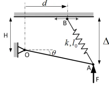
Figure 1.Variable Stiffness Mechanism.
2 System description
This section gives a detailed description of the variable stiff -ness concept, the overall system, its incorporation in a vehi-cle suspension, and the resulting system dynamic model.
2.1 Variable stiffness concept
The variable stiffness mechanism concept is shown in Fig. 1. The Lever arm OA, of length L, is pinned at a fixed point O and free to rotate about O. The spring AB is pinned to the lever arm at A and is free to rotate about A. The other end B of the spring is free to translate horizontally as shown by the double headed arrow. It is also free to rotate about point B. Without loss of generality, the external force F is assumed to act vertically upwards at point A. d is the horizontal distance of B from O. The idea is to vary the overall stiffness of the system by letting d vary passively under the influence of a horizontal spring-damper system (not shown in the figure). Let k and l0be the spring constant and the free length of the
spring AB respectively, and ∆the vertical displacement of the point A. The overall free length∆0of the mechanism is
defined as the value of∆when no external force is acting on the mechanism.
2.2 Mechanism description
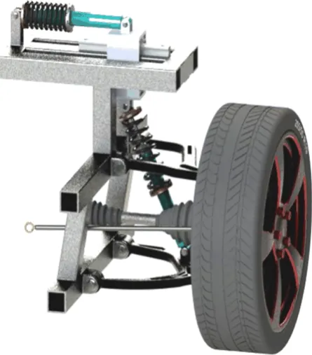
The suspension system considered is shown in Fig. 2. The schematic diagram is shown in Fig. 3. The model is com-posed of a quarter car body, wheel assembly, two spring-damper systems, road disturbance, and lower and upper wishbones. The points O, A, and B are the same as shown in the variable stiffness mechanism of Fig. 1. The horizon-tal control force u controls the position d of the control mass mdwhich, in turn, controls the overall stiffness of the
Figure 2.Variable Stiffness Suspension System.
The assumptions adopted in Fig. 3 are summarized as fol-lows:
1. The lateral displacement of the sprung mass is ne-glected, i.e only the vertical displacement ys is
consid-ered.
2. The wheel camber angle is zero at the equilibrium posi-tion and its variaposi-tion is negligible throughout the system trajectory.
3. The springs and tire deflections are in the linear regions of their operating ranges.
2.3 Equations of motion Let
q=
ys
θ
d
, (1)
be defined as the generalized coordinates. The equations of motion, derived using Lagrange’s method, are then given by
M(θ) ¨q+C(θ,θ˙)+B(θ) ˙q−K(q)+G(θ)
=e3,3u+Wd(θ)dr (2)
where
M(θ)=
ms+mu+md mulDcosθ 0
mulDcosθ Ic+mul2Dcos
2θ 0
0 0 md
,
Figure 3.Quarter Car Model
C(θ,θ˙)=−mulDθ˙2sinθw(θ),
w(θ)=
1 lDcosθ
0
,
B(θ)=
bt btlDcosθ 0
btlDcosθ btl2Dcos2θ+bsgθ b2sgdθ
0 bs
2gdθ bsgd
,
gd(d,θ)=
(d−lAcosθ)2
H2+d2+l2
A−2lAd cosθ−2HlAsinθ ,
gdθ(d,θ)=
2lA(d−lAcosθ) (d sinθ−H cosθ)
H2+d2+l2
A−2lAd cosθ−2HlAsinθ ,
gθ(d,θ)=
l2
A(d sinθ−H cosθ)
2
H2+d2+l2
A−2lAd cosθ−2HlAsinθ ,
K(q)=
kt(ρt−1) (ys+lDsinθ)
kt(ρt−1) lDcosθ(ys+lDsinθ)
ks(ρs−1)(d−lAcosθ)
+
0
ks(ρs−1) lA(d sinθ−H cosθ)
0
G(θ)=
ms+mu+md
mulDcosθ
0
g,
Wd(θ)=
kt(ρt−1) bt
ktlD(ρt−1) cosθ btlDcosθ
0 0
,
dr=
" r ˙r
#
.
r(t) is the road displacement signal. It is a function of the road profile and the vehicle velocity. The termsρsandρt
charac-terize the compression of the vertical strut and tire springs respectively. They are defined as the instantaneous length di-vided by its free length.
Properties
The following properties of the dynamics given in Eq. (2) are exploited in subsequent analyses:
1. The inertia matrix M(θ) is symmetric, positive definite. Also, since each element of M(θ) can be bounded be-low and above by positive constants, it folbe-lows that the eigenvalues, hence the singular values of M(θ) can also be bounded by constants. Thus, there exists m1,m2∈ R+
such that
m1kxk2≤xTM(θ)x≤m2kxk2 and (3)
1 m2
kxk2≤xTM−1(θ)x≤ 1 m1
kxk2, ∀x∈R2 (4)
2. C(θ,θ˙) can be upper bounded as follows
C(θ,θ˙)
≤c1θ˙
2, c
1∈R+. (5)
Also, there exist a matrix Vm(θ,θ˙) such that C(θ,θ˙)=
Vm(θ,θ˙) ˙q and
xT 1
2 ˙
M(θ)−Vm(θ,θ˙)
!
x=0, ∀x∈R2 (6)
The property in Eq. (6) is the usual skew symmetric property of the Coriolis/centripetal matrix of Lagrange dynamics (Lewis et al., 2004).
3. The damping matrix B(θ) is symmetric and positive semi definite. Also, there exists positive definite matri-ces B and ¯B such that
0<xTBx≤xTB(θ)x≤xTBx¯ , ∀x∈R2. (7)
4. The stiffness vector K(q) is Lipschitz continuous, i.e. there exists a positive constant k2such that
kK(q1)−K(q2)k ≤k2kq1−q2k. (8)
5. The unique static equilibrium point q0=
h
ys0 θ0 d0
iT
of the undisturbed system is known and is given by
K(q0)−G(θ0)+e3,3u0=0. (9)
3 System analysis
This section presents the finite-gain stability analysis of the system described in the previous section. The disturbance dr
in Eq. (2) is assumed to be unknown a priori but bounded in the sense that dr∈ L2. As a result, robust optimal control
is considered in which the gain of the system is optimized under worst excitations: Ball and Helton (1989); Helton and James (1999); Soravia (1996); van der Schaft (1996). The following definition describes the notion of stability used in the subsequent analyses.
Finite-GainL-Stable (van der Schaft, 1996) Consider the nonlinear system
˙x= f (x,w)
z=h(x) (10)
where x∈ Rn,w∈ Rp,z∈ Rmare the state, input, and output
vectors, respectively. The system in Eq. (10), with the map-ping MH:L
p
e→ Lme, is said to be finite-gainL-stable if there
exist real constantsγ,β≥0 such that
kMH(w)kL≤γkwkL+β, (11)
wherek.kL denotes theL norm of a signal, and Lne is the
extendedLspace defined as
Lne={χ|χτ∈ Ln,∀τ∈[0,∞)} (12) whereχτis a truncation ofχgiven as
χτ(t)=
( χ
(t) 0≤t≤τ
0 t> τ. . (13)
For the purpose of this paper, the L2-space is
consid-ered, hence the finite-gainL-stability condition in Eq. (11) is rewritten as (van der Schaft, 1996)
kMH(w)k2≤γkwk2+β, (14)
wherek.k2denotes theL2norm of a signal given by
kχk2=
∞
Z
0
χT(t)χ(t)dt
1 2
. (15)
γ∗=inf{γ| kM
H(w)k2≤γkwk2+β}is the gain of the system,
and, in the case of linear quadratic problems, is the H∞norm
Eq. (14) is satisfied for some β >0. This solution is ap-proached from the perspective of dissipative systems (Ball and Helton, 1989; van der Schaft, 1996). The following def-inition describes the concept of dissipativity with respect to the system in Eq. (10).
Dissipativity The dynamics system Eq. (10) is dissipative with respect to a given supply rate s(w,z)∈ R, if there ex-ists an energy function V(x)≥0 such that, for all x(t0)=
x0and tf≥t0,
V(x(tf))≤V(x(t0))+
tf
Z
t0
s(w,z)dt, ∀w∈ L2. (16)
If the supply rate is taken as
s(w,z)=γ2kwk2− kzk2, (17)
then the dissipation inequality in Eq. (16) implies finite-gain L-stability (van der Schaft, 1996), and the system is said to beγ-dissipative. The dissipativity inequality is then written as
˙
V≤γ2kwk2− kzk2. (18)
3.1 Performance objective
As usual with suspension systems designs, the performance criterion is expressed in terms of the ride comfort, suspension deflection, and dynamic tire force. The performance vector
z=
ω1ycba ω2ysd
ω3ydtf
(19)
characterizes the ride comfort, suspension deflection, and road holding performances, whereω1,ω2, andω3are the
re-spective user specified performance weights for car body ac-celeration ycba, suspension deflection ysd, and dynamic tire
force ydtf. The ride comfort is characterized by the car body
acceleration ¨ys which is approximated using the following
high gain observer (Khalil, 1996):
εη˙=Aη+b˙ys, η(0)=0
ycba=1εcTη
(20)
where
A= "
−1 1 −1 0
#
, b=
" 1 1
#
, c=
" 0 1
#
.
The L2-norm of the car body acceleration can be upper bounded as (Khalil, 1996)
kycbak2≤c1k˙ysk2≤c1k˙ek2, (21)
where
c1=
2λ2
max(P)kbk2kck2
λmin(P)
and P is the solution of the Lyapunov equation PA+ATP+I=
0, which is obtained as
P=1
ε
" 1 12
1 2
3 2
#
.
The suspension deflection is given as
ysd(t)=
q l2
s(0)−l2s(t)
=n
d(0)2−d(t)2−2H x (sinθ(0)−sinθ(t))
−2x (d(0) cosθ(0)−d(t) cosθ(t))}12 (22)
≤h 0 k41 k42
i
|y0s−ys|
|θ−θ0|
|d−d0|
, (23)
Using the Cauchy-Schwarz inequality, ysd(t) can be upper
bounded as
ysd(t)≤k4kek, (24)
where k41,k42,and k4 are positive constants, and
k4≥
q k2
41+k 2 42.
The dynamic tire force is characterized using the tire deflection and is given by
ydtf(t)=yu(0)−yu(t)
=y0s−ys+lD(sinθ0−sinθ) (25)
≤h 1 k5 0
i
|y0s−ys|
|θ−θ0|
|d−d0|
, (26)
where k5 is a positive constant. Using the Cauchy-Schwarz
inequality, ydtf(t) can be upper bounded as
ydtf≤
q 1+k2
5 kek=k6kek. (27)
Finally, theL2-norm of the performance vector in Eq. (19)
can be upper bounded as
kzk2≤φ1k˙ek2+φ2kek2 (28)
where
φ1=ω1c1
3.2 Constant stiffness case
Now, consider the constant stiffness case in which the control mass is locked at a given position d. As a result, the overall stiffness is constant for the entire trajectory of the system. For this case, the dynamics in Eq. (2) reduces to
M1(θ) ¨q1+C1(θ,θ˙)+B1(θ) ˙q1−K1(q1)+G1(θ)=w, (29)
where
M1=M1:2,1:2,C1=C1:2,
K1=K1:2,B1=B1:2,1:2,
w=Wd1dr,Wd1=Wd1:2,1:2
Here, the corresponding dynamics of the control mass has been eliminated.
Let
e1=q1−q01 (30)
where
q01=
" ys0
θ0
#
(31)
be the equilibrium value of the reduced state vector q1. After
using the Mean Value Theorem, the closed-loop dynamics in Eq. (29) is expressed as
M1¨e1+Vm1˙e1+K1e1+B1˙e1=w (32)
where
K1=−
∂K1
∂q1
q
1=ζ1
+ ∂G1
∂q1
q
1=ζ2
ζ1,ζ2,∈ Ls(q01,q1).
Lemma 1: The matrix
P= "
I m1I
m1I M1
#
(33)
is positive definite, where m2
1< λmin{M1}.
Proof. Letλbe an eigenvalue of P. It follows thatλ∈ R, since P is symmetric. The characteristic polynomial of P is given by
p(λ)=det{λI−P} (34)
=detn(λ−1) (λI−M)−m21Io (35)
Now, λ=1⇒p(λ)=m4
1,which implies that λ=1 is NOT
an eigenvalue of P. Suppose without loss of generality that
λ,1, then
p(λ)=(λ−1)2det
λ2−λ−m2 1
λ−1 I−M
. (36)
Thus there exists an eigenvalueλmof M such that
λ2−λ−m2 1
λ−1 =λm, (37)
which implies that
λ=1
2
1+λm±
q
(1+λm)2−4
λm−m21
, (38)
from which it follows thatλ >0. Since P is symmetric, the conclusion follows.
Remark It follows from Rayleigh-Ritz Inequality that
p1
χ
2
≤χTPχ≤p2
χ
2
, (39)
where p1=λmin{P}, and p2=λmax{P}.
Theorem 1. If the matrix
H1=
1 2
−Kˆ1−KˆT1 −KT1 −m1M−11B1
−K1−m1
M−11B1
T
−2 ˆB1
, (40)
where
ˆ
K1=m1M−11K1−
c1k˙ek
2 I (41)
ˆ
B1=B1− m1+
c1k˙ek
2 !
I, (42)
is negative definite along the entire trajectory of the closed-loop error system in Eq. (32), then theL2-norm of the per-formance vector in Eq. (19) can be upper bounded as
kzk2≤γ1kwk2+β1, (43)
where
γ1=
φσp2
p1h1
, (44)
β1=
√ 2φp2
p p1h1
, (45)
and
φ=max{φ1,φ2} (46)
σ=σmax
(" m1M−11
I #)
(47)
h1=|λmin{H1}|. (48)
Proof. Consider the energy function
V(e1,˙e1)=
1 2χ
T
1Pχ1, (49)
where
χ1=
"
e1
˙e1
#
Taking time derivative of Eq. (49) and using the skew sym-metric property in Eq. (6) yields
˙
V=−˙eT1(B1−m1I) ˙e1−e˙1TK1e1+˙e1Tw+m1eT1M
−1 1 w
−m1eT1M
−1
1 Vm˙e1−m1eT1M
−1
1 B1˙e1−m1eT1M
−1
1 K1e1. (51)
Using the property in Eq. (5) yields
˙
V≤χT1H1χ1+χT1
" m1M−11
I #
w, (52)
which after using the negative definiteness of H1yields
˙ V≤ −h1
χ1 2 +σ χ1
kwk. (53)
Take W(t)=pV(χ1).When V(χ1),0, ˙W=V˙/(2 √
V) yields
˙ W≤ − h1
2p2
W+ σ 2√p1
kwk. (54)
When V(χ1)=0, it can be verified (Khalil, 1996) that
D+W≤ σ 2√p1
kwk, (55)
where D+denotes the upper right hand differentiation opera-tor. Hence
D+W≤ − h1 2p2
W+ σ 2√p1
kwk (56)
for all values of V(χ1). Next using comparison (Lemma 3.4, Khalil, 1996) yields
W(t)≤W(0) exp −h1t 2p2
!
+ σ 2√p1
t
Z
0
kwkexp −h1(t−τ) 2p2
!
dτ, (57)
which implies that
χ1(t)
≤ rp 2 p1 χ1(0)
exp −
h1t
2p2 ! + σ 2p1 t Z 0
kwkexp −h1(t−τ) 2p2
!
dτ. (58)
Thus
χ1(t)
2≤
σp2
p1h1
kwk2+ √
2p2
p p1h1
χ1(0)
.
Lastly, after using the inequality in Eq. (28), theL2-norm of the performance vector can be upper bounded as
kzk2≤φσp2 p1h1
kwk2+ √
2φp2
p p1h1
χ1(0)
. (59)
Remark TheL2-gain of the system decreases with increas-ing h1. This means that the more the negative definiteness
of H1, the more the disturbance rejection achievable by the
system.
The following theorem gives the bounds on achievableγ.
Theorem 2. Given an attenuation levelγ, and provided that the performance weights are selected to satisfy the sufficient condition
φ=max{φ1,φ2}<
p
h1, (60)
then the closed loop error system in Eq. (32) isγ-dissipative with respect to the supply rate
s(w,z)=γ2kwk2− kzk2 (61) if
γ≥ 0.5σ
p h1−φ2
. (62)
Proof. Consider the energy storage function in (49). Tak-ing first time-derivate, and addTak-ing and subtractTak-ing the supply rate yields
˙
V≤χTH1χ+χTLw
≤γ2kwk2− kzk2+χTH1χ
−γ2
w−L
Tχ
2γ2
2 + 1 4γ2χ
TLLTχ+φ2 χ 2
≤γ2kwk2− kzk2+χT H1+ φ2+
σ2
4γ2
! I
! χ
≤γ2kwk2− kzk2− h1−φ2−
σ2
4γ2
! χ 2 (63)
After using the inequality in Eq. (62)
˙
V≤γ2kwk2− kzk2, (64) which implies that the closed loop error system in Eq. (32) is
γ-dissipative.
Remark The inequality in Eq. (62) shows that the level of performance achievable is limited by the amount of damp-ing and stiffness available in the system. It will be shown in subsequent sections that this limit can be pushed further by using a variable stiffness architecture. The lower bound in Eq. (62) is termed “best-case-gain”. It defines the smallest gain achievable by the system.
The stiffness and damping matrices K1, and B1 contain
bounded functions of state and uncertain dynamic param-eters which range between bounded values. Thus the best-case gain of the system with constant stiffness can be lower bounded as
γ
1≥
0.5σ q
h∗
1−φ2
where h∗
1 is the smallest positive number larger than the
smallest singular value of H1, andγ1 is termed the “robust
best-case gain”.
3.3 Passive variable stiffness case
Here, the control mass is allowed to move under the influ-ence of a restoring spring and damper forces. There is no external force generator added to the system. As a result, the system response is purely passive. Let kuand bube the spring
constant and damping coefficient of the restoring spring and damper respectively. The control force u is then given by
u=−bud˙−ku(d−l0d), (66)
and the resulting dynamics of the control mass is given by
mdd¨+bud˙+ku(d−l0d)+ks(ρs−1)(d−x cosθ)
+bs
2gdθθ˙+bsgdd˙=0, (67) and the static equilibrium equation for the control mass is given by
ku(d0−l0d)+ks(ρs0−1)(d0−x cosθ0)=0, (68)
where d0is the equilibrium position of the control mass, and
l0dis the free length of the restoring spring. Let
ed=d−d0 (69)
be the displacement of the control mass from its equilibrium position. Substituting Eq. (69) into Eq. (67) and using the Mean Value Theorem yields
md¨ed+BTd˙e+K T
de=0, (70)
where e= " e1 ed # , (71) Bd= 0 bs
2gdθ
bsgd+bu
, (72) Kd= 0
ks∂(ρs−1)(d∂θ−x cosθ)
θ∈L
s(θ0,θ)
ku+ks
∂(ρs−1)(d−x cosθ) ∂d
d∈Ls(d0,d)
. (73)
Now, consider the energy function
V2(e,˙e)=.χT2P2χ2, (74)
where,
χ2=
" e ˙e # , (75) and
P2=
"
I mI
mI M #
(76)
is positive definite, with m2< λmin{M}. Taking the first time
derivative of Eq. (74), and following a similar procedure as in the constant stiffness case in the previous section yields
˙
V2≤γ2kwk2− kzk2+χT2H2χ2, (77)
where
H2=
1 2
−Kˆ −KˆT −KT−mM−1B
−K−mM−1BT
−2 ˆB
, (78)
ˆ
K=mM−1K−c1k˙ek
2 I, (79)
ˆ
B=B− m1+
c1k˙ek
2 !
I, (80)
and
K=−∂K
∂q
q=ζ1+
∂G ∂q q=ζ2
,ζ1,ζ2,∈ Ls(q0,q). (81)
Now, the robust best-case gain of the system with a passive variable stiffness is given by
γ
2≥
0.5σ q
h∗
2−φ 2
. (82)
where h∗2is the smallest positive number larger than smallest singular value of H2. Here, the spring constant ku, and the
damping coefficient buof the control mass restoring
spring-damper system can be chosen such thatγ
2< γ1. Thus, a
bet-ter performance can be achieved just by letting the stiffness vary naturally using a spring-damper system. This claim is supported subsequently by experimental and simulation re-sults. This is a very appealing result due to its practicability. No additional electronically controlled or force generating device is required, only mechanical elements like the spring and damper are used.
4 Experiment
Figure 4.Quarter Car Experimental Setup.
the 2011 Honda PCX scooter front suspensions. The road generator is a simple slider-crank mechanism actuated by Smartmotor®SM3440D geared down to a ratio of 49 : 1 us-ing CMI®gear head P/N 34EP049. Three accelerometers are attached, one each to the quarter car frame, the wheel hub, and the road generator. Data acquisition was done using the MATLAB data acquisition toolbox via NI USB-6251. Exper-iments were performed for the passive case, where the hori-zontal strut is just a passive spring-damper system, and also for the fixed stiffness case, where the top of the vertical strut is locked in a fixed position. This position is the equilibrium position of the passive case when the system is not excited.
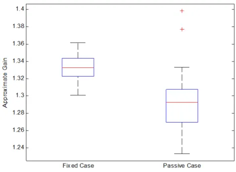
Two tests were carried out; sinusoidal, and drop test. For the sinusoidal test, the road generator is actuated by a con-stant torque from the DC motor. As a result, the quarter car frame moves up and down in a sinusoidal fashion. To facili-tate a good comparison of the observations, the “approximate gain” of the system defined as
γ2=
RT
0 z(t) 2dt
RT
0 r(t)
2dt, (83)
where z(t) is the signal of interest, and r(t) is the road accel-eration signal, is numerically computed. The signals of inter-est are the frame acceleration and tire deflection acceleration signals. The experimental procedure was repeated multiple times in order to verify the repeatability of the experiment. Figures 5 and 6 show the box plots of the approximate gain distributions for the fixed stiffness and passive variable stiff -ness cases. It is seen that the worst and best case gains for the fixed stiffness are higher than those of the passive vari-able stiffness case, thereby confirming the analytical result obtained earlier that the variable stiffness achieves better dis-sipation.
Figure 5.Box Plot: Car Body Acceleration.
Figure 6.Box Plot: Tire Deflection Acceleration.
For the drop test, the suspension system was dropped to the ground1 from a fixed height (6 inches from the equilibrium position and the wheel was not in contact with the ground). The resulting quarter car body acceleration and tire deflection accelerations were recorded. This test examines the response of the system to initial conditions. Figures 7 and 8 shows the car body acceleration responses and tire deflection accelera-tion responses for the fixed and variable stiffness cases.
Table 1 shows the approximate gains for the sinusoidal and the rms values of the drop test. The approximate gains of the sinusoidal test given in the table are the mean values of the multiple experiments.
5 Simulation
In order to study the behavior of the quarter car system at full scale as well as responses like suspension deflection, which
1Here the ground is non accelerating as against the sinusoidal
Figure 7.Drop Test: Car Body Acceleration.
Figure 8.Drop Test: Tire Deflection Acceleration.
Figure 9.Solidworks Quarter Car Model.
were difficult to measure experimentally, and excitation sce-narios that are difficult to implement experimentally, realistic simulations were carried out using MATLAB Simmechanics Second Generation. First, the system was modeled in Solid-works as shown in Fig. 9. Next, the Simmehanics model was developed. The mass/inertia properties used are the ones gen-erated from the Solidworks model. The vertical strut and tire
Table 1.RMS/Approximate gain values of experimental results. CBA: Car Body Acceleration. TDA: Tire Deflection Acceleration.
Fixed Passive
Drop (RMS) CBA (g) 0.4543 0.3710 TDA (g) 0.2746 0.2396
Sinusoidal (Gain) CBA 0.6220 0.5170 TDA 1.3316 1.2944
Table 2.Dynamic parameter values.
Parameter Value
ms 315 kg
mu 37.5 kg
bs 1500 N m−1s−1
ks 29 500 N m−1
kt 210 000 N m−1
damping and stiffness used are the ones given in the “Re-nault M´egane Coup´e” model (Zin et al., 2004). The values are given in Table 2.
5.1 Time domain simulation
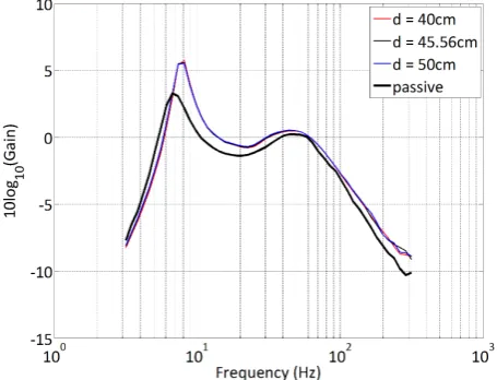
In the time domain simulation, the vehicle traveling at a steady horizontal speed of 40 mph is subjected to a road bump of height 8 cm. The Car Body Acceleration, Sus-pension Deflection, and Tire Deflection responses are com-pared between the constant stiffness and the passive vari-able stiffness cases. For the constant stiffness case, the con-trol mass was locked at three different locations (d=40 cm, d=45.56 cm and d=50 cm). The value d=45.56 cm is the equilibrium position of the control mass. Next, a simulation is performed for the passive case. The results are reported in Figs. 10, 11 and 12 which are the the car body acceleration, suspension deflection, and tire deflection responses, respec-tively. Figure 13 shows the position history of the control mass for the passive variable stiffness case.
5.2 Frequency domain simulation
Figure 10.Time Domain Simulation: Car Body Acceleration.
Figure 11.Time Domain Simulation: Suspension Deflection.
Figure 12.Time Domain Simulation: Tire Deflection.
Figure 13.Time Domain Simulation: Control Mass Position.
G( jω)= v u u u u u u u u u u u u u u u u u u u u u u u u u u t
2πN/ω Z
0
z2dt
2πN/ω Z
0
A2sin2(ωt) dt
, (84)
where z denotes the performance measure of interest which is taken to be car body acceleration, suspension deflection, and tire deflection. The closed loop system is excited by the si-nusoid r=A sin(ωt), t∈[0, 2πN/ω], where N is an integer big enough to ensure that the system reaches a steady state. The corresponding output signals were recorded and the ap-proximate variance gains were computed using Eq. (84). Fig-ures 14, 15, and 16 show the variance gain plots for the car body acceleration, suspension deflection, and tire deflection respectively. The figures show that the variable stiffness sus-pension achieves better vibration isolation in the human sen-sitive frequency range (4–8 Hz) (ISO 2631-1, 1997), and bet-ter handling beyond the tire hop frequency (>59 Hz) (Fialho and Balas, 2002).
6 Conclusion
The design, analysis, and experimentation of the passive case of a new variable stiffness suspension system is presented. Using a detailedL2-gain analysis based on the concept of
Figure 14.Frequency Domain Simulation: Car Body Acceleration.
Figure 15.Frequency Domain Simulation: Suspension Deflection
Figure 16.Frequency Domain Simulation: Tire Deflection.
Nomenclature
kvk Euclidean norm of the vector v
yu Vertical displacement of the unsprung
mass
ys Vertical displacement of the sprung mass
hu Half distance between points C and D
ls Vertical strut length
l0s Natural length of vertical strut
lD Length of the lower wishbone
H Height of the control mass from the pivot point of the lower wishbone
x Distance between points O and A along the lower wishbone
kt, bt Tire spring constant and damping coeffi
-cient
ks, bs Vertical Strut stiffness and damping coeffi
-cient
ku, bu Control(Horizontal) Strut stiffness and
damping
ms, mu, md Sprung, unsprung and control masses
Ic Moment of inertia of control arm.
λmin{A} The minimum eigenvalue of the matrix A
λmax{A} The maximum eigenvalue of the matrix A
σmin{A} The minimum singular value of the matrix
A
σmax{A} The maximum singular value of the matrix
A
Ai: j,k:l The sub-matrix of matrix A formed by
rows i to j and columns k to l
Ai: j The sub-matrix of matrix A formed by
rows i to j and all columns tr{A} The trace of the matrix A det{A} The determinant of the matrix A
Ls(q1,q2) The set of points that lie on the line
seg-ment joining the vectors q1and q2
I Identity matrix
ei,n The i-th column of the identity matrix of
dimension n
R The set of real numbers
Re{α} The real part of the complex numberα
Edited by: A. M¨uller
References
Alkhatib, R., Jazar, G. N., and Golnaraghi, M. F.: Optimal design of Passive Linear Suspension Using Genetic Algorithm, J. Sound Vib., 275, 665–691, 2004.
Anubi, O. M., Crane, C., and Ridgeway, S.: Design and Anal-ysis of a Variable Stiffness Mechanism, in: Proceedings IDETC/CIE2010. ASME 2010 International Design Engineering Technical Conferences & Computers and Information in Engi-neering Conference, 2010.
Ashfak, A., Saheed, A., Abdul-Rasheed, K. K., and Jaleel, J. A.: Design, Fabrication and Evaluation of MR Damper, International Journal of Aerospace and Mechanical Engineering, 1, 27–33, 2011.
Ball, J. and Helton, J.: H∞control for nonlinear plants: Connections
with differential games, in: Proceedings of the 28th Conference on Decision and Control, Tampa, Florida, 956–962, 1989. Butsuen, T.: The Design of Semi-active Suspensions for
Automo-tive Vehicles, Ph.D. thesis, Massachussets Institute of Technol-ogy, 1989.
Do, A.-L., Sename, O., and Dugard, L.: An LPV Control Approach for Semi-active Suspension Control with Actuator Constraints, in: 2010 American Control Conference, 2010.
Evers, W.-J., Teehuis, A., van der Knaap, A., Besselink, I., and Ni-jmeijer, H.: The Electromechanical Low-Power Active Suspen-sion: Modeling, Control, and Prototype Testing, J. Dyn. Syst.-T. ASME, 133, 041008-1–041008-9, 2011.
Fialho, I. and Balas, G. J.: Road Adaptive Active Suspension De-sign Using Linear Parameter-Varying Gain-Scheduling, IEEE T. Contr. Syst. T., 10, 43–54, 2002.
Helton, J. and James, M.: Extending H∞Control to Nonlinear
Sys-tems: Control of Nonlinear Systems to Achieve Performance Ob-jectives, Society for Industrial Mathematics, 1987.
ISO 2631-1, I.: International Organization of Standardization. Me-chanical Vibration and Shock – Evaluation of Human Exposure to Whole Body Vibration. Part 1: General Requirement, Geneva, 1997.
Jerz, J.: Variable stiffness suspension system, uS Patent 3,559,976, 1971.
Karnopp, D.: Active damping in road vehicle suspension systems, Vehicle System Dynamics, 12, 291–316, 1983.
Karnopp, D. and Heess, G.: Electronically controllable vehicle sus-pensions, Vehicle Syst. Dyn., 20, 207–217, 1991.
Karnopp, D., Crosby, M., and Harwood, R.: Vibration control using semi-active force generators, J. Eng. Ind., 96, 619–626, 1974. Khalil, H.: Nonlinear systems, Prentice hall New Jersey, 3rd Edn.,
1996.
Kobori, T., Takahashi, M., Nasu, T., Niwa, N., and Ogasawara, K.: Seismic response controlled structure with active variable stiff -ness system, Earthq. Eng. Struct. D., 22, 925–941, 1993. Lewis, F. L., Dawson, D. M., and Abdallah, C. T.: Robot
Manipula-tor Control, Theory and Practice, Marcel Dekker, Inc., 2nd Edn., 2004.
Liu, Y., Matsuhisa, H., and Utsuno, H.: Semi-active vibration isola-tion system with variable stiffness and damping control, J. Sound Vib., 313, 16–28, doi:10.1016/j.jsv.2007.11.045, 2008.
NHTSA: New Passenger Car Fleet Average Characterisitcs, http:
//www.nhtsa.gov/cars/rules/cafe/NewPassengerCarFleet.htm, 2004.
Schoukens, J., Pintelon, R., Rolain, Y., and Dobrowiecki, T.: Fre-quency Response Function Measurements in the Presence of Nonlinear Distortions, Automatica, 37, 939–946, 2001. Soravia, P.: H∞ Control for Nonlinear Systems: Differential and
Viscosity Solutions, SIAM Journal of Control and Optimization, 34, 1071–1097, 1996.
Stack, A. J. and Doyle, F. J.: A Measure for Control Relevant Non-linearity, in: American Control Conferencel, Seattle, 2200–2204, 1995.
Sung, K., Han, Y., Lim, K., and Choi, S.: Discrete-time fuzzy slid-ing mode control for a vehicle suspension system featurslid-ing an electrorheological fluid damper, VTT Symp., 16, 798–808, 2007. Tseng, H. E. and Hedrick, J. K.: Semi-Active Control Laws – Opti-mal and Sub-OptiOpti-mal, Vehicle Syst. Dyn., 23, 545–569, 1994. Valasek, M. and Kortum, W.: Nonlinear control of semi-active
road-friendly truck suspension, in: Proceedings AVEC 98, 275–280, Nagoya, 1998.
Valasek, M. and Kortum, W.: The Mechanical Systems Design Handbook; Modeling, Measurement and Control, chap. Semi-Active Suspension Systems II, CRC Press LLC, 2001.
van der Knaap, A.: Design of a Low Power Anti-Roll/Pitch System for a Passenger Car, Ph.D. thesis, Delft University of Technology, 1989.
van der Knaap, A. C. M., Teerhuis, A. P., Tinsel, R. B. G., and Ver-shuren, R. M. A. F.: Active Suspension Assembly for a Vehicle, International Patent No. 2008/049845, 2008.
van der Schaft, A. J.:L2-Gain and Passivity Techniques in Nonlin-ear Control, Springer, Berlin, 1996.
Venhovens, P. J. T. and van der Knaap, A. C. M.: Delft Active Sus-pension (DAS), Background Theory and Physical Realization, Smart Vehicles, 139–165, 1995.
Williams, R. A.: Automotive active suspensions. Part 1: basic prin-ciples, in: Proceedings of IMechE, 211, 415–426, 1997. Williams, R. A., Best, A., and Crawford, I. L.: Refined low
fre-quency active suspension, in: Proceedings of IMechE Interna-tional Conference, 285–300, 1993.
Youn, I. and Hac, A.: Semi-active suspension with adaptive capa-bility, J. Sound Vib., 180, 475–492, 1995.