Steps for the Solution of Faddeev Integral Equations in Configuration
Space
George Rawitscher1,aand Walter Gl¨ockle2
1 Physics Department, University of Connecticut, Storrs, CT 06268 USA
2 Institut f¨ur Theoretische Physik II. Ruhr Universit¨at Bochum, D-44780, Bochum, Germany
Abstract. Faddeev equations in configuration space for three-atom scattering processes that have previously been formulated in integral form allowing for additive and nonadditive forces, are now examined in terms of their numerical properties for a ”toy-model” case. The numerical implementa-tion is based on a spectral decomposiimplementa-tion in terms of Chebyshev polynomials. The potential for high accuracy of this method, of the order of 6 to 8 significant figures is one of the main motivations for the present investigation.The object of the equations areT−functions, that are the product of wave functions times potentials, that decay to zero in all directions. The driving and coupling terms are based on the two-bodyt−matrices, which describe the two-body correlations in each arrangement. The preferred form for both the driving term and the integral kernel terms is of a hybrid nature, the x−dependence is expanded into Chebyshev polynomials, and they−dependence is given in terms of a Fourier series. The numerical properties of the driving term are examined in detail, and the integral kernel is left for a subsequent analysis.
1 Introduction
Our form of the equations have been modeled after the corresponding integral equations in momentum space [1], and a preliminary account is available [2], [3]. A numerical evaluation of these equations has up to now not been implemented and progress in that direction for a simplified example will be described. An accu-racy of 6 to 8 significant figures is envisaged by using a spectral expansion method in terms of Chebyshev polynomials [4], [5] for solving integral equations in configuration space. A basic ingredient is the integral of the two-body scatteringt−matrix over a given func-tion, which can now be obtained with a fast algorithm with an accuracy of more than eight significant figures [6].
The object of the equations are T−functions,
T(x, y),that are the product of wave functions times potentials, that decay to zero in all directions. The nu-merical properties of the drivingD(x, y) term of the coupled integral equations for the T- functions have now been established in the present investigation, and they serve as a guide for the choice of the algorithm for the solution of the overall coupled equations. The numerical evaluation of the latter is left for a future investigation. The most promising equation structure that emerges is a hybrid method, in which the be-havior of T(x, y) in the x−variable is obtained by a spectral expansion into Chebyshev polynomials [4], while the behavior in the y−variable is expressed by
a
means of a Fourier integral representation. A Malfliet-Tjon potential is used for the two-body interaction, the three body potentials are set to zero, spin is ig-nored, all orbital angular momenta are set to zero, and the particles are taken to be identical. In arrangement 1 the x−vector is the displacement vector of particle 3 to particle 2, and they−vector is the displacement vector from particle 3 to the center of mass of particles 2 and 3.
The basic equation to be solved in this toy model example is
T(x, y) =D(x, y)+ Z Z
K(x, x′, y, y′)T(x′, y′)dx′dy′,
(1) where D(x, y) is the driving term and K is the inte-gration kernel, and where T(x, y) is the quantity to be calculated. The double integral will be denoted as
KT in what follows. The directions of the vectors x andyhave already been integrated out. We find that a convenient form for the driving term is
D(x, y) =
Z ∞
0
DF(q, x)j
0(qy)dq (2) whereDF(q, x) can be expressed in terms of a function
TF(q, x)
DF(q, x) = (2π)−5/2(4q/3q 0)
1
xTF(q, x), (3)
whose x− dependence can be obtained very conve-niently by means of expansions into Chebyshev poly-nomials. Hereq0(q) is the momentum of the incident
DOI:10.1051/epjconf/201005012
(outgoing) particle on the target in the ground (ex-citedεt) state of energy−|ε0|. The quantity TF(q, x) is obtained in terms of various nested integrals involv-ing the two-bodyt−matrix at the energyεt.The latter is the two-body energy of particles 2 and 3 obtained by subtracting from the total energy the kinetic energy of the particle 1 with momentumq.Whenqis nearq0,
εtis close to−|ε0|, andTF has a pole. This, and other poles for excited bound states of the two-body system in the integral 2 can be handled by subtraction, as will be shown.
The purpose of the present report is to describe the procedure for obtaining numerical values for the functionTF(q, x), and analyze it numerical properties so as to determine the most suitable ansatz for solving the integral equation (1), to be carried out in a future investigation.
2 The equations for
D
(
x, y
)
The driving term, given by Eq. (41) of Ref. [2] is com-posed of a direct term Dc =t1PcΦ1 and an exchange termDac=t1PacΦ1, wherePc andPacare the cyclic ant anti-cyclic permutation operators. The cyclic (or direct) term is
Dc≡t1P12Φ1= 1
(2π)3 Z
d3q eiq·(y−y′)
hx|τ|x ′iΦ(x′′,y′′)d3x′d3y′
(4)
where the vectorsx′′andy′′are related to the vectors x′ andy′ according to
x′′=−1 2x
′ −y′; y′′=3 4x
′−1 2y
′ (5)
For the anticyclic caset1P13Φ1 one has x′′=−12x′+y ′; y ′′=−34x′−1
2y ′ (6)
HereΦis the product of the ground state target wave function and the plane wave of the incident particle,
Φ(x′′,y′′) = (2π)−3/2eiq0·y′′u
0(x′′) (7) where q0 is the momentum of the particle 1 incident on the center of mass of particles 3 and 2. For aℓ= 0 bound state of the target particle the wave function is given by
u0(x′′) =√1 4π
1
x′′u0(x
′′) (8)
whereu0(x′′) is the radial partial wave function. Fur-therτ is the two-body T−matrix for particles 2 and 3, whose partial wave expansion is given by
<x|τ|x′ >= 1
x x′ 1 4π
X
l
τl(εq;x, x′)Pl(ˆx·xˆ′). (9)
We take as zero the angular momenta inτ ,and obtain
Dc= (2π)−9/2 Z
d3q eiq·(y−y′)ei q0·ρ0
u0(ρ2) √
4πρ2 1 4π
1
x x′τ0(εq;x, x
′)d3x′ d3y′ (10)
where
ρ0= 3 4x
′
−12y′; ρ2= 1 2x
′+y′. (11)
We now set to zero the following angular momenta
eiq·(y−y′)
→j0(q|y−y′|) (12)
eiq0·ρ0→j
0(q0|ρ0|).
Replacing the spherical Bessel function j0(z) by
F0(z)/z, whereF0(z) = sin(z) we obtain
Dc= (2π)−9/2 Z
d3q j
0(q|y−y′|)
F0(q0ρ0)
q0ρ0
u0(ρ2) √
4πρ2 1
4π
1
x τ0(εq;x, x
′)x′ dx′dΩ
x′y′2dy′ dΩy′ (13) The integrations over the solid angle dΩx′y′ can be accomplished by making y′the polar axis and by us-ing ρ2
0 = (9/16)x′2+ (1/4)y′2−(3/4)x′y′cosθx′y′, hence dΩx′ = 2πsinθx′y′dθx′y′ = −2πd(cosθx′ y′) =
4πρ0 dρ0
(3/4)x′y′.As cosθx′ y′decreases from +1 to−1,ρ0 in-creases from (3/4)x′−(1/2)y′to (3/4)x′+(1/2)y′,i.e.,
dρ0increases positively asθx′y′ increases from 0 toπ. Further using (ρ2)2=−(4/3) (ρ0)2 +x′2+ (4/3)y′2 and defining the function ¯u0(q0, x′, y′)
¯
u0(q0, x′, y′) =
Z ρ0max
ρ0min
F0(q0ρ0) u0(ρ2)
ρ2
dρ0. (14)
The integration overdΩy′ follows from
ρ3dρ3 =−y y′ d(cosθy,y′), where ρ3 =y−y ′, with the result
Z
j0(qρ3)dΩy′ = 2π yy′q
Z y+y′ |y−y′|
F0(qρ3)dρ3
= 4π
yy′q2sin(qy) sin(qy
′). (15)
It is noteworthy that in the above result the depen-dence inyandy′is separable. After defining the func-tionuS(q0, q, x′)
uS(q0, q, x′) =
Z ∞
0 ¯
u0(q0, x′, y′) sin(q y′)dy′ (16) and
TF(q0, q, x) = Z xmax
0
one finally obtains
Dc= 2 1/2π−3 3 q0 x y
Z ∞
0
TF(εq, x) sin(qy)dq (18)
The simple form of Eq. (18) is due to the separability of Eq. (15). Asqchanges the corresponding two-body energyεq in τ0 changes correspondingly according to
εq= 3 4q
2
0− |εb| − 3 4q
2 (19)
whereεbis the binding energy of the two nucleons that form the target nucleus. In the appendix it is argued that the contribution from the anti-cyclic case toDis identical to that of the cyclic case, and hence
D(x, y) =Dc+Dac=k 1
xy
Z ∞
0
TF(εq, x) sin(qy)dq.
(20) with
k=2 3/2π−3
3q0
3 Numerical results for the driving term.
The two nested integrals ¯u0(q0, x′, y′), Eq. (14) and
uS(q0, q, x′), Eq. (16); and the solution of the L−S integral equation (17) forTF(q0, q, x), as described in Ref. [6], are carried out numerically using the spectral expansion techniques, first described in Ref. [4] and later used for several applications [7]. A retrospective of this work is presented in Ref. [8]. The bound state functionu0(x), Eq. (8) is obtained with the iterative method described in Ref. [9]. The Malfliet-Tjon po-tential, already multiplied by the factor 2µ/~2 is of the form
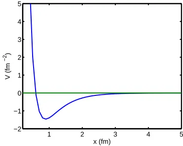
V(r) = (35.15907∗exp(−3.11∗r) −13.933932∗exp(−1.55∗r))/r
in units of f m−2, as illustrated in Fig.(1). In order to suppress the singularity at the origin, the poten-tial is replaced by a soft core at distances less than
rcut= 0.2 f m given in terms of a second order poly-nomial in powers of r, matched to the potential in the vicinity of rcut as described previously. The re-sulting values of V at r = 0, 0.2, and 10 f m are approximately 231,43.3 and −2.6 ×10⁻⁷f m−2, re-spectively. The bound state occurs at an energy of −(0.1005443)2f m−2. The bound state wave function
u(r) has a value of 2.8×10⁻⁹ atr= 140f m, but the calculation of the bound state energy is done out to a distance or 350f m, using the procedure described in Ref. [9]. The momentum of the incident particle, described by they−coordinate, has the value ofq0= 2f m−1.
The integration procedure consist in dividing the in-tegration domain into partitions, expanding the inte-grand in each partition into a fixed set of Chebyshev
1 2 3 4 5
−2 −1 0 1 2 3 4 5
x (fm)
V (fm
−
2)
Fig. 1. The Malfliet-Tjon potential used throughout this text. It is already multiplied by the factor 2µ/~2
polynomials (17 is standard), adaptively choosing the size of each partition such that the last three expan-sion coefficients have a magnitude less than the im-posed accuracy parameter tol, and then performing the integrals over the Chebyshev polynomials using the standard matricesSLandSR[4]. In the numerical applications [7] it was found that the accuracy of the final result was comparable to the value oftol, which in the present calculation has the value of 10−8. Al-lowing for a loss of accuracy of two significant figures, it is expected that the accuracy ofTF(q0, q, x) is of the order of 1 : 10−6. Since the two-body τ−matrix has a pole at the bound state energy, which occurs when
q=q0,special care has to be exercised in the vicinity of that point, as will be described in a forthcoming publication.
3.1 The xandq dependence ofTF
Numerical results forTF(x, q),Eq. (17) are illustrated in the figures below for several values ofq,both smaller and larger than q0.
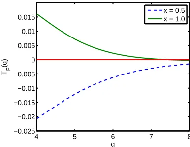
The figures show considerable changes inTFasqvaries, however, as q increasesTF decreases rapidly. This is also illustrated in fig. (4), that shows the dependence ofTF as a function ofqfor a fixed value ofx= 1.0f m The singularity at q=q0 is clearly visible. The curve of TF(x, q) versusq forx= 0.5 f mis similar to that shown in Fig.(4), only its sign is opposite, and the magnitude is approximately a factor two larger. The rate of decrease of TF with increasingq can be seen from Fig.(5).
For the expansion of TF(q, x) into Chebyshev poly-nomials it is advantageous to divide the domain ofx
into partitions, rather than expanding the whole do-main all at once. This is illustrated in Fig. (6) for
0 1 2 3 4 5 −1
−0.5 0 0.5 1 1.5 2 2.5
x
TF
(x)
q = 1, q
0=2
Fig. 2.The dependence ofTF onxfor the values ofq (in
units of f m−1) indicated in the figure. The bound state
pole occurs atq0.
0 1 2 3 4 5
−0.025 −0.02 −0.015 −0.01 −0.005 0 0.005
x
TF
(x)
q = 2.4, q
0 = 2
Fig. 3. Same as Fig.(2) forq > q0.
0 1 2 3 4
−1 −0.5 0 0.5 1 1.5 2
q
T
F
(x=1.0,q)
Fig. 4.Dependence ofTF onqfor the fixed value ofx=
1.0f m.The subscript 1234 ofTFindicates that this figure
is a composite of four q−partitions, whoseq−boundaries are: 1) from 0.01 to 1.00, 2) from 1.00 to 1.99, 3) from 2.01 to 2.4, and 4) from 2.4 to .4, all in units off m−1.
The results for partitions 5 and 6, with 4 ≤ q ≤ 6, and 6≤q≤8, respectively, are displayed in Fig. (5).
4 5 6 7 8
−0.025 −0.02 −0.015 −0.01 −0.005 0 0.005 0.01 0.015
q
TF
(q)
x = 0.5 x = 1.0
Fig. 5. The decrease ofTF for large values ofq, between
4 and 8f m−1
0 5 10 15 20 25 30
10−15 10−10 10−5 100 105
order of Chebyshev pol.
Cheb. exp. coeffs of T
F
0−>10 0−>0.2 0.2−>0.5 1−>2 2−>5 5−>10
Fig. 6. The convergence of the Chebyshev expansion coefficients of TF(q = 1, x) for various sizes of the x−partitions. The global expansion in the whole interval 0≤x≤10f mconverges less rapidly than than the con-vergence in each of the five partitions into which the whole x−interval is divided, as described in the legend.
the expansion. That is not the case for the global ex-pansion fromx= 0 to x= 10.Expansions into other functions, such as Laguerre or Legendre polynomials or Fourier expansions converge much less slowly than the Chebyshev expansion.
3.2 The xandy dependence of the driving term
In order to obtain the y−dependence of D(x, y) it is necessary to carry out the integration R
0 5 10 15 20 25 30 −0.5
−0.4 −0.3 −0.2 −0.1 0 0.1 0.2
y
T
F
(x=1,y)
q = 0.01 to 4
Fig. 7. The functionTF(x, y) forx= 1 obtained by
inte-grating Eq.(20) overq.The result is obtained by applying Eq.(21) to the four q−partitions 1 to 4 described in the caption to Fig. (4).The contribution from the pole singu-larity 1.99≤q≤2.01, shown in Fig.(8), is too small to be visible.
Z +1 −1
T2n+1(¯q)
sin(¯qy) p
1−q¯2 dq¯= (−) nπ J
2n+1(y) Z +1
−1
T2n(¯q)
cos(¯qy) p
1−q¯2 dq¯= (−) nπ J
2n(y). (21) where the J is a Bessel function. So, for each fixed value ofxone expandsTF(q, x) into Chebyshev poly-nomials Tn(q)
TF(q, x) = N X
n=0
cn(x) pTn(q)
1−q2 (22) and hence
Z qmax 0
TF(q, x) sin(qy)dq= N X
n=0
cn(x) (−)nπ J2n+1(y). (23) The range ofqis divided into partitions, and by means of Eqs. (21) the integrals over q are performed for each partition, and subsequently the results from each partition are added. The result for the fixed value of
x= 1 is shown in Fig. (7) The followingq−partitions were used: 0.01→1,1→1.990,2.01→2.4,2.4→4. The singular partition 1.99 → 2.10 was left out in Fig. (7), and calculated separately. Its contribution is of the order of 10−3,which is too small to been seen in the figure.
3.3 Contribution from the pole term.
The contribution from the partition that contains the pole was calculated in two different ways. One, which uses a addition and subtraction method around the pole, similarly to what is done in the momentum rep-resentation, denoted as analytical method, and the
0 5 10 15 20 25 30
−6 −4 −2 0 2 4x 10
−3
y
T F
pole(x=1,y)
T
F pole, analytical
T F pole, numerical
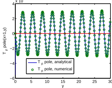
Fig. 8. Comparison of a rigorous numerical-analytical evaluation of TF(pole)(x, y),defined in Eq.(24),with a nu-merical method based on an expansion ofTF into
Cheby-shev polynomials, according to Eq.(21). The good agree-ment between the two methods shows the power of Cheby-shev expansions.
other, denoted as the numerical method, based on Eq. (21), is treated as described above. In that case theq -domains from 1.99→2.0 and from 2.0→2.01 are de-composed into 17 Chebyshev polynomials, each. Both methods gave very similar results, as shown in Fig. (8), which illustrates
TF(pole)(x, y) =
Z qo+tmax
qo−tmax
TF(εq, x) sin(qy)dq. (24)
The good agreement shows that the ”brute-force” nu-merical method, based on Eq.(21) is robust, even in the vicinity of a singularity, but the more theoretical method, based on addition and subtraction of a known singularity, is preferable if high accuracy is desired.
4 The integral kernel
K
The integral equation for the functionT(x, y), accord-ing to Eq. (41) of Ref. [2] is
T =t1PΦ1+t1G0PT =D+KT, (25) The first term is the driving term and the second term contains the integral K=t1G0PT over the unknown functionT, which will be the object of the present sec-tion. First the general structure of the nested integrals will be described, and the numerical realization is left to a separate publication.
Remembering that P contains a direct and an ex-change term (cyclic and anti-cyclic permutations), mak-ing the transformation between different sets of Jacobi coordinates implied by P, and using the descriptions of the Green’s functiong0 given by
gl(x, x′, εq) =
−p1 q
whereFℓandGℓare the regular and irregular Riccati-Bessel functions for angular momentum numberℓone obtains withℓ= 0 the expression
KT(x, y) = 1 (2π)3
Z
d3q eiq·(y−y′′) 1
4πxx′τ0(x, x ′, ε
q)
1 4πx′x′′g0(x
′x′′, ε
q)d3x′x′′2dx′′dϕx′′y′′d3y′′ Z
dt T(ρ′′2, ρ′′0) + Z
dt T(ρ′′5, ρ′′4)
(27)
In the above dt=−d(cosθx′′y′′), the vectorsρ2′′, ρ0′′ are defined in Section 2, and ρ′′
5, ρ′′4 are defined the same way for the anticyclic permutation. Similarly as was shown for the calculation of the driving term, the cyclic and anti cyclic parts are the same for theℓ= 0 case, and hence the two integrals in the third line of Eq. (27) are equal. By transforming to the variableρ′′ 0 one findsdt= 2ρ′′0 dρ′′0
(3/4)x′′y′′,and as a result the third line of Eq. (27) is
TI(x′′, y′′) = Z −1
1
dt T(ρ′′ 2, ρ′′0) +
Z −1 1
dt T(ρ′′ 5, ρ′′4) = 4
(3/4)x′′y′′T¯(x
′′, y′′) (28)
where
¯
T(x′′, y′′) =Z ρmax
ρmin
ρ′′
0 dρ′′0 T(ρ′′2, ρ′′0) (29) and whereρ2 = [−(4/3) (ρ0)2 +x′ 2+ (4/3)y′ 2]1/2 andρmin=|(3/4)x′′−(1/2)y′′|andρmax= (3/4)x′′+ (1/2)y′′.The integration ofT
I(x′′, y′′) overdx′′should include the Green’s function g0(x′, x′′, εq) in Eq. (27) and is denoted asI1
I1(q, x′, y′′) =
Z ∞
0
dx′′ T¯(x′′, y′′)g0(x′, x′′, εq) (30)
The integration of I1 over dy′′ should take into ac-count the factor sin(qy′′) which arises from the inte-gration over the direction ofq in the first line of Eq. (27)
I2(q, x′) =
Z ∞
0
sin(qy′′)I1(q, x′, y′′)dy′′. (31)
This quantity still has to be integrated over x′, with inclusion of the two-body τ0−matrix in Eq. (27)
I3(q, x) =
Z ∞
0
τ0(x, x′, εq)I2(q, x′)dx′. (32) Combining all these expressions one finally obtains for
KT
KT(x, y) =c 1
xy
Z ∞
0
sin(qy)I3(q, x)dq. (33)
This expression is of the same format as Eq. (20) for the driving term, rendering the overall equation forT
T(x, y) = 1
xy
Z ∞
0
[kTF(εq, x) +c I3(q, x)] sin(qy)dq, (34) with
c= 4
3π2 (35)
This suggests that a convenient ansatz forT is
T(x, y) = 1
xy
Z ∞
0
L(q, x) sin(qy)dq, (36)
in which case the two-variable equation for the un-knownLwould be
L(q, x) =kTF(εq, x) +c I3(q, x) (37) The first term is the driving term, the second be-comes an integral over T in view of the sequence of the nested integrals, Eqs. (28) through (33). If further thex−dependence ofL(q, x) is expanded into Cheby-shev polynomials
L(q, x) = pmax
X
p=1 N+1
X
n=1
a(np)(q)Tn(p)(x) (38)
where the x−domain is divided into partitions 1,2, ..pmax then, in view of Eq. (37), one obtains a set of coupled equations for the expansion coefficients
a(np)(q) that has to be solved numerically. Here p de-notes the partition number,Tn(p)(x) is the Chebyshev polynomial linearly transformed to the boundaries of each partition. The realization of such a scheme is left to a future study, however the structure of the equa-tions to be solved (Eq. (37)) is again of the hybrid form, in the variablesxandq.
5 Summary and Conclusions
highly oscillatory and decreases only slowly with dis-tance, as illustrated in Fig.(7), while the Fourier coeffi-cients for the driving term are not strongly oscillatory, and decrease reasonably rapidly with theq−variable, as illustrated in Fig. (4). The calculation of the driving term required three nested integrals, which were per-formed numerically, while the calculation of the inte-gral kernel requires four nested inteinte-grals, to be carried out in a future study. The proposed set of of coupled equations to be solved for the Fourier expansion co-efficients of the function T(x, y) were described near Eq. (37). The imaginary parts of the Greens functions were left out in the present exploratory study and the numerical evaluation of the integration kernel together with the solution of the coupled equations for the ex-pansion coefficients will also be left for a subsequent study.
In conclusion, in order to demonstrate that our ap-proach for solving the Faddeev integral equations in configuration space is feasible and can be rendered very accurate by means of spectral expansions into Chebyshev polynomials, the first step was to numer-ically evaluate and examine the driving term of the integral equation for the T−function for the ”toy-model” case described here, and suggestions for how to formulate and solve the corresponding integral equa-tion for theT−function have been presented.
References
1. D. H¨uber, H.Kamada, H.Witala, W.Gl¨ockle, Acta Phys. Pol. 28 (1997) 1677; W.Gl¨ockle, H.Witala, D.H¨uber, H.Kamada, J.Golak, Phys. Rep.274, 107 (1996);
2. W. Gloeckle, and G. Rawitscher, ”Three-atom scattering via the Faddeev scheme in configuration space”, physics/0512010 at arxiv.com;
3. W. Gloeckle, and G. Rawitscher, Nucl. Phys. A 790,(2007) 282c -285c ;
4. R. A. Gonzales, J. Eisert, I Koltracht, M. Neu-mann and G. Rawitscher, J. of Comput. Phys.134, (1997) 134-149 ; R. A. Gonzales, S.-Y. Kang, I. Koltracht and G. Rawitscher, J. of Comput. Phys. 153, (1999) 160-202;
5. A. Deloff,,Ann. of Phys.322, (2007) 1373 ; 6. G. Rawitscher and W. Gloeckle, Phys. Rev.A77,
(2008) 01207;
7. G.H. Rawitscher G.H. et al., J Chem. Phys., 111, (1999) 10418 -10426; G. Rawitscher, Kang, S.-Y. and I. Koltracht, I., J. Chem. Phys., 118, (2003) 9149-9156; G. Rawitscher, and I. Koltra-cht, Computing in. Sc. and Eng.,7, (2005) 58 ; G. Rawitscher, J. Phys. A: Math. Theor. 42, (2009) 015201;
8. George H. Rawitscher, Operator Theory: Adv. and Applic., 203 (2009 Birk¨auser Verlag, Basel/Switzerland), 409-426 ;