A Discrete-Time Algorithm for the Resolution of the Nonlinear Riccati Matrix Differential Equation for the Optimal Control

(1)

Published online March 10, 2014 (http://www.sciencepublishinggroup.com/j/ajce) doi: 10.11648/j.ajce.20140202.11

A discrete-time algorithm for the resolution of the

Nonlinear Riccati Matrix Differential Equation for the

optimal control

Tahar Latreche

Doctorate student at Constantine University, Algeria, B.P. 129 Salem Lalmi, 40003 Khenchela, Algeria

Email address:

[email protected]

To cite this article:

Tahar Latreche. A Discrete-Time Algorithm for the Resolution of the Nonlinear Riccati Matrix Differential Equation for the Optimal Control. American Journal of Civil Engineering. Vol. 2, No. 2, 2014, pp. 12-17. doi: 10.11648/j.ajce.20140202.11

Abstract:

The Riccati Matrix Differential Equation (RMDE) is an interesting equation in different fields of science and engineering practice. In fact, that the arithmetic solution for this matrix differential equation in the general case of varying-time matrices is very difficult to find. The literature offers the solution of this differential equation in the case of dependant constant matrices (i.e. invariant-time matrices). The present approach is an approximate discrete-time method for the resolution of the matrix differential equation of Riccati in the general case of varying-time (dependant of time) matrices; the method in fact, is a discrétisation of the exact matrix solution, that evaluates for any so small step of time, and which is function of the solution of the preceding step of time and the constitute equation matrices. The proposed algorithm is verified, for a controlled structure under Modified El-Centro earthquake by a comparison with the same uncontrolled structure, which constitutes by a two Degrees Of Freedom (2DOF) system. The results of this comparison offer good differences between the controlled and the uncontrolled systems.

Keywords:

Riccati Matrix Differential Equation, Discrete-Time Algorithm, Varying-Time Matrices, Optimal Control, Nonlinear Quadratic Regulator

1. Introduction

The Optimal Control is a field of science which is interesting by different branches of science and engineering such that Economy, Electronics, Civil Engineering, Mechanical Engineering, Communication Engineering, Aeronautical Engineering, Robotics and Quantum Physics. The Linear and the Nonlinear Quadratic Regulators are universal methods for the resolution of the problem of the controlled systems subjected to signals or earthquakes. The determination of the control signals or the output feedback gain in the case of closed-loop, conduct to the resolution of the Riccati Matrix Differential Equation, which is in the general case nonlinear. The arithmetic or theoretical solution of this equation is in fact very difficult to find. As a conclusion of literature cited bellow [1-15], one can find that there are be theoretical solutions for this equation in the cases of constant solution, or in the more than that, in the case of invariant with time matrices (i.e. in the linear state space equation); but in fact, there’s no accurate method or algorithm for the resolution of this equation in the general case of nonlinear state space equation (i.e. the

(2)

needed against the pseudo-monotone solution in the case of linearity.

2. NLQR with Full State Feedback

As we know that, the dynamic equilibrium equation of a system can be transformed to the state space formulation

(1) With, and are state space matrices, such that is a nonlinear or a dependent of time matrix. Define the Hamiltonian function, which is a scalar function of time, as

Figure 1. The El-Centro earthquake ⁄

(2) and are weighting matrices. In order to minimizing the cost function involves taking the variation of the Lagrangian with respect to , and , it follows that

!

" # 0 %&' 0 !

( # ) 0 0 * !

&+ # 0

,

(3)

To solve the set of simultaneous equations in Eq. (3), _& is generally unknown in real time control. Therefore, the value of _& is taken to be very large. Now substituting Eq. (2) into Eq. (3), it follows that

Figure 2. Controlled and uncontrolled displacements of the first floor

!

" # 0

!

( # ) ) 0

!

&+ # 0

, 4)

Solving for in the third equation in Eq. (4), we can obtain

) - ₍₅₎

Substituting Eq. (5) into the first equation in Eq. (4), and solving for and , gives the system of equations

Figure 3. Controlled and uncontrolled velocities for the first floor

. / 0 _- ₎ 1 . / (6)

(3)

Figure 4. Controlled and uncontrolled accelerations for the first floor

0 _- ₎ 1 2 (7)

is called Hamilton Matrix. Suppose that

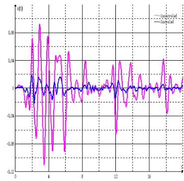
Figure 5. Controlled and uncontrolled displacements for the second floor

3 (8) Substituting Eq. (8) into Eq. (5), we obtain

) - ₃ ₍₉₎

But 3 is unknown, and we can see how can we obtain for a discrete time in the next section.

Differentiating Eq. (8) with respect to time, and substituting and by their expressions (Eq. 6) and

by Eq. (8), we can obtain

Figure 6. Controlled and uncontrolled velocities for the second floor

3 3

3 3 - ₃

) 3 3

Simplifying this equation, and dividing by , we obtain

3 3 3 ) 3 - ₃ ₍₁₀₎

Which is called the Matrix Differential Riccati Equation (RMDE), and its solution, 3 is needed to compute the output feedback .

Figure 7. Controlled and uncontrolled accelerations for the second floor

3. Discrete-Time Solution of the RMDE

Integrating the Eq. (6) with respect to time, from ₄ to

(4)

67 . 45

45 / ) 67 . 4

4 / 8 2 9

!:;<

!: (11)

Suppose that ∆> ₄₅ ) ₄, a so small step of time for the raison that the Hamiltonian Matrix elements vary constantly.

Suppose that

Figure 8. Controlled and uncontrolled forces vs. displacements for the first floor

2 ? 2? (12)

Then the equation (11) can be expressed as

67 . 45

45 / ) 67 . 4

4 / 24∆> 2⁄ A4

Or, by elevate it to a power

. 45

45 / B

C:∆ ⁄ . 4

4 / (13)

The matrix B C:∆ ⁄ _{has the same dimensions like} 2_?_,

then we can compute it by the Taylor series, as

A345 B C:∆ ⁄ BD: ∑ D:

:

4! G

4H* (14)

We can suppose that ₄ ₄ and ₄ ₄ , and we subdivide A3₄₅ on four equal dimensions matrices, such as

A345 IA3_A345 A345

45 A345 J (15)

As we suppose that 3 - (Eq. 8), then we can obtain for any step of time, using the subdivision of Eq. (17)

345 A345 4 A345 4 A345 4 A345 4 - (16)

Multiplying rightly the nominator and the denominator of the right side of Eq. (18) by ₄- , we would obtain then

345 A345 34 A345 A345 34 A345 - (17)

For K 0, we can obtain

3 A3 3* A3 A3 3* A3 - (18)

Such that 3_* represent the given initial condition at

K 0 (i.e. at 0).

Table 1. The comparison between controlled and uncontrolled maximal responses

Nonlinear Analysis

Uncontrolled Disp., Vel. And Acc.

Controlled Disp., Vel. And Acc.

First Floor 0,110 1,051 12,160 0,022 0,330 5,678

Second Floor 0,063 0,722 8,349 0,008 0,243 5,229

% of differences Disp., Vel. and Acc. successively

First Floor 0,801 0,686 0,533

Second Floor 0,879 0,664 0,374

The Eq. (19) and (20) represent the discrete-time solution for the Nonlinear Matrix Differential Equation of Riccati. Note that, as we take a so small step of time ∆>, as the solution being more exact and accurate.

Figure 9. Controlled and uncontrolled forces vs. displacements for the second floor

4. Demonstration Example

A tow degrees of freedom system, subjected to El-Centro Earthquake shown by the Figure 1, with the property matrices of the state space formulation (Eq. 1) which are given by

0₂-0_M ₂-L_{N 1}

O 0₂- P

(5)

0.25 and, K K 2S in the case of elastic domain and, K K_T K 3⁄ in the case of plastic domain. The stiffness model is considered as a bilinear model with the given data. The step of time is ∆> 0.02 BVW79 and the elastic displacement is considered as X_*

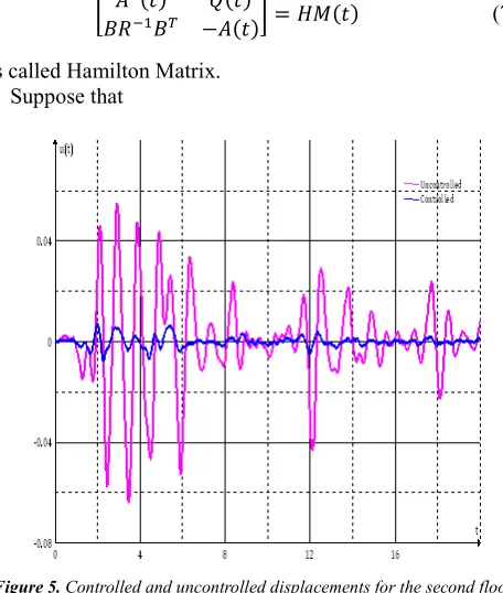
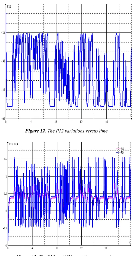
0.002 B BY . The controlled and uncontrolled displacements, velocities and accelerations of the first floor are shown by the Figures 2, 3 and 4 successively, while that concern the second floor are shown by the Figures 5, 6 and 7 successively. The hysteresis Force-Displacement for the first and the second floor, for controlled and uncontrolled systems, are shown successively by the Figures 8 and 9. The matrix solution of the Riccati equation in this example is then 4 [ 4, symmetric and its four equal blocs are too, symmetric. The variations of its elements versus time are shown by the Figures 10, 11, 12, 13 and 14.

Figure 10. The P11 and P22 variations versus time

Figure 12. The P12 variations versus time

(6)

5. Conclusion

The optimal control in general is an interesting branch of engineering, and it is conduct to the resolution the classical Riccati matrix differential equation. The theoretical solution of the nonlinear matrix differential equation of Riccati is really difficult to find. There were exact solutions for this equation in the linear case; but there is no solution for the nonlinear case. This algorithm presents a good approximation of the solution in the general case, of dependent of time matrices of the state space formulation and the weighting matrices. When the solution is found, one can deduct the output control feedback, which works to reduce the responses of the structure subjected to earthquakes. This algorithm in fact, being more and more precise and accurate only when the step of time of reading the signal, analyzing the structure, deducting the output feedback and practicing it by mean of actuators, is so small as possible. The application of this algorithm for 2 % of a second time step, for a two degrees of freedom nonlinear system, gives a good results such as the responses of the structure (Displacements: about 80 %, Velocities: 70 % and Accelerations: 40 %, reduction) as shown in Table 1. and the concerned Figures. The acted forces at any floor are reduced for about 70 % for controlled structure compared to that uncontrolled one, and this is because closed-loop control of the displacements and also, because the effect of the nonlinearity of the structure taken for a chosen plastic stiffness as a third of the elastic stiffness; but in reality, the plastic stiffness is less than this value, which makes the differences between the controlled and uncontrolled responses increase. The Figures concern the solution of Riccati equation elements versus time show the effect of the nonlinearity of the equation constituents’ matrices, while in linearity shown as pseudo-monotones.

References

[1] Anderson, B. D. O. et Moore, J. B., (1971). Linear optimal control. First Edition, Prentice-Hall, Inc.

[2] Anderson, B. D. O. et Moore, J. B., (1979). Optimal Filtering. First Edition, Prentice-Hall, Inc.

[3] Anderson, B. D. O. et Moore, J. B., (1989). Optimal control, linear quadratic methods. First Edition, Prentice-Hall, Inc.

[4] Arfiadi, Y., (2000). Optimal passive and active control mechanisms for seismically excited buildings. PhD Thesis, University of Wollongong

[5] Astolfi, A. et Marconi, L., (2008). Analysis and design of nonlinear control systems. First Edition, Springer Publishers

[6] Elliott, D. L., (2009). Bilinear control systems. First Edition, Springer Publishers

[7] Grewal, M. S. et Andrews, A. P., (2008). Kalman Filtering: Theory and practice. Third Edition, John Wiley and Sons, Inc.

[8] Grune, L. et Pannek, J., (2011). Nonlinear model predictive control. First Edition, Springer Publishers

[9] Isidori, A., (1999). Nonlinear control systems 2. First Edition, Springer Publishers

[10] Marazzi, F., (2002). Semi-active control for civil structures: Implementation aspects. PhD Thesis, University of Pavia

[11] Preumont, A., (2002). Vibration control of active structures: An Introduction. Second Edition, Kluwer Academic Publishers

[12] Vér, I. L. et Beranek, L. L., (2006). Noise and vibration control engineering. First Edition, John Wiley and Sons, Inc.

[13] William, S. L., (2011). Control system: Fundamentals. Second Edition, Taylor and Francis Group, LLC

[14] William, S. L., (2011). Control system: Applications. Second Edition, Taylor and Francis Group, LLC