R E S E A R C H
Open Access
Modelling urban networks using
Variational Autoencoders
Kira Kempinska
1,2*and Roberto Murcio
1*Correspondence: [email protected]
1Centre for Advanced Spatial
Analysis (CASA), University College London, London, UK
2Alphamoon Ltd, Wrocław, Poland
Abstract
A long-standing question for urban and regional planners pertains to the ability to describe urban patterns quantitatively. Cities’ transport infrastructure, particularly street networks, provides an invaluable source of information about the urban patterns generated by peoples’ movements and their interactions. With the increasing availability of street network datasets and the advancements in deep learning methods, we are presented with an unprecedented opportunity to push the frontiers of urban modelling towards more data-driven and accurate models of urban forms. In this study, we present our initial work on applying deep generative models to urban street network data to create spatially explicit urban models. We based our work on Variational Autoencoders (VAEs) which are deep generative models that have recently gained their popularity due to the ability to generate realistic images. Initial results show that VAEs are capable of capturing key high-level urban network metrics using low-dimensional vectors and generating new urban forms of complexity matching the cities captured in the street network data.
Keywords: Variational autoencoders, Urban modelling, Street networks
Introduction
Temporal and spatial patterns of human interactions shape our cities making them unique, but, at the same time, create universal processes that make urban structures com-parable to each other. A long-standing effort of urban studies focuses on the creation of quantitative models of the spatial forms of cities that would capture their essential characteristics and enable data-driven comparisons. There have been several attempts at studying urban forms using quantitative methods, typically based on complexity theory or network science (Arcaute et al.2016; Barthélemy and Flammini2008; Murcio et al.
2015; Buhl et al.2006; Cardillo et al.2006; Masucci et al.2009; Strano et al.2013). The approaches create an abstract representation of an urban form to derive its key quanti-tative characteristics. Although theoretically robust, the abstractions might often be too simplistic to capture the full breadth and complexity of existing urban structures.
With the increasing availability of urban street network data and the advancements in deep learning methods, we are presented with an unprecedented opportunity to push the frontiers of urban modelling towards more data-driven and accurate urban models. Street networks are a ubiquitous element at every urban area and a robust proxy for pop-ulation density, jobs and housing accessibility and environmental features (Zhao et al.
part of a superimposed pattern developed by local and regional governments. In that sense, this paper could provide urban planners with the capabilities of creating not one, but thousands of street configurations, where different actors can test a variety of urban scenarios.
In this study, we present our initial work on applying deep generative models to urban street network data to create spatially explicit models of urban networks. We based our work on Variational Autoencoders (VAEs) trained on images of street networks. VAEs are deep generative models that have recently gained their popularity due to the ability to gen-erate realistic images. VAEs have two fundamental qualities that make them particularly suitable for urban modelling. Firstly, they can condense high dimensional images of urban street networks to a low-dimensional representation which enables quantitative compar-isons between urban forms without any prior assumptions. Secondly, VAEs can generate new realistic urban forms that capture the diversity of existing cities. In this work, we use image representation of street networks since images encodebothtopological and spatial network information. Street network images could be parsed to graphs, if desired, using road parsing algorithms (Li et al.2018; Chu et al.2019; Máttyus et al.2017).
In the following sections, we show our experiments based on urban street networks from Open Street Map (OSM). The results indicate that VAE trained on the OSM data is capable of capturing critical high-level urban metrics using low-dimensional vectors. The model can also generate new urban forms of structure matching the cities captured in the OSM dataset. All code and experiments for this study are available athttps://github.com/ kirakowalska/vae-urban-network.
Methodology and dataset Variational autoencoder
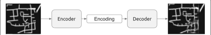
Variational Autoencoders (VAEs) have emerged as one of the most popular deep learn-ing techniques for unsupervised learnlearn-ing of complicated data distributions. VAEs are particularly appealing because they compress data into a lower-dimensional representa-tion which can be used for quantitative comparisons and new data generarepresenta-tion. VAEs are built on top of standard function approximators (neural networks) efficiently trained with stochastic gradient descent (Kingma and Welling2014). VAEs have already been used to generate many kinds of complex data, including handwritten digits, faces, house numbers, and predicting the future from static images. In this work, we apply VAEs to street net-work images to learn low-dimensional representations of street netnet-works. We use the representations to make quantitative comparisons between urban forms without making any prior assumptions and to generate new realistic urban forms (Fig.1).
A variational autoencoder consists of an encoder, a decoder, and a loss function. The
encoderis a neural network. Its input is a datapointx, its output is a hidden representation
z, and it has weights and biasesθ. The goal of the encoder is to ’encode’ the data into a latent (hidden) representation spacez, which has much fewer dimensions that the data. This is typically referred to as a ’bottleneck’ because the encoder must learn an efficient compression of the data into this lower-dimensional space. The encoder is denoted by
qφ(z|x).
The decoder is another neural network. Its input is the representationz, it outputs a data point x, and has weights and biases φ. The decoder is denoted by pφ(x|z). The decoder ’decodes’ the low-dimensional latent representationzinto the datapointx. Information is lost in the process because the decoder translates from a smaller to a larger dimensionality. How much information is lost? The information loss is measured using the reconstruction log-likelihood logpφ(x|z). The measure indicates how effectively the decoder has learned to reconstruct an input imagexgiven its latent representationz.
Theloss functionof the variational autoencoder is the sum of the reconstruction loss, given by the negative log-likelihood, and a regularizer. The total loss is the sum of losses
N
i=1liforNdatapoints, where the loss functionlifor datapointxiis:
li(θ,φ)= −Ez∼qθ(z|xi)[ logpφ(xi|z)]+KL(qθ(z|xi)||p(z)) (1)
The first term is the reconstruction loss or expected negative log-likelihood of the
i-th data point. This term encourages the decoder to learn to reconstruct the data. Poor reconstruction of the dataxfrom its latent representationzwill incur a large cost in this loss term. The second term is a regularizer that we introduce to ensure that the distri-bution of the latent valueszapproaches the prior distributionp(z)specified as a Normal distribution with mean zero and variance one. The regularizer is the Kullback-Leibler divergence between the encoder’s distributionqθ(z|x)andp(z). It measures how closeqis top. The regularizer ensures that the representationszof each data point are sufficiently diverse and distributed approximately according to a normal distribution, from which we can easily sample.
The variational autoencoder is trained using gradient descent to optimize the loss with respect to the parameters of the encoder and decoderθandφ.
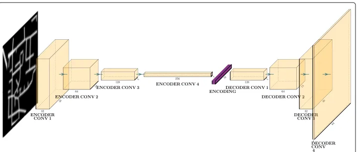
In our work, we selected Convolutional Neural Networks (CNNs) (Fukushima1980; LeCun et al.1990) as the encoder and decoder architectures. CNNs are deep learning architectures that are particularly well-suited to image data (LeCun et al.1995; Krizhevsky et al.2014) as they consider the two-dimensional structure of images and scale well to high-dimensional images. We tested several CNN architectures and finally chose a net-work architecture in Fig.2with the encoder and the decoder architectures consisting of four convolutional blocks, each with a convolutional and a rectified linear unit (ReLU) layer (which introduces non-linearity to the network). The architecture takes as input an image of size 64×64 pixels, convolves the image through the encoder network and then condenses it to a 32-dimensional latent representation. The decoder then reconstructs the original image from the condensed latent representation. We implemented the variational autoencoder using PyTorch library for Python.
Street network data
Fig. 2Variational autoencoder architecture. Yellow blocks represent convolutional blocks (convolutional layer followed by ReLU layer) with dimensions corresponding to their output dimensions. The purple block is the learnt embeddingz
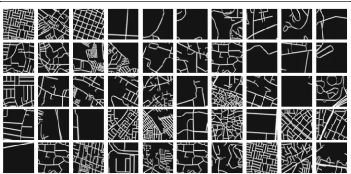
from the Global Human Settlement database1. We saved the street networks as images and, as the Variational autoencoders required images to have a fixed spatial scale, we extracted a 3×3kmsample from the centre of each city image and resized it to a 64×64 pixels binary image. The final dataset contained 12,479 binary images of 64×64 pixels, which we split into 80% training and 20% testing datasets. During model training, we aug-mented the training dataset by randomly cropping and flipping the images horizontally. Figure3shows images for randomly selected cities.
Results
Reconstruction quality
The variational autoencoder was trained to minimise the loss function defined in (1). The training is equivalent to minimising the image reconstruction loss, subject to a regularizer. We can inspect the training quality by visually comparing reconstructed images to their original counterparts. Figure4shows several examples of reconstructed images of urban street networks. As observed in the examples, the trained autoencoder performs well at reconstructing the overall shape of road networks and their main roads. The quality of the reconstruction drops for very dense road networks when only the overall network shape is captured by the autoencoder (see the leftmost image in Fig.4). The observation suggests that variational autoencoders are better suited for reconstructing images with wide patches of pixels with similar properties rather than narrow stretches such as roads.
Urban networks comparison
The trained autoencoder learnt mapping from the space of street network images (64×64 or 4,096 dimensions) to a lower dimensional latent space (32 dimensions). The latent representation stores all the information required to reconstruct the original image of the street network, so it is effectively a condensed representation of the street network that preserves all its connectivity and spatial information. In the lack of well-defined simi-larity metrics of urban networks, this paper uses the condensed representations as vectors of street network features. Hereafter, we call the vectorsurban network vectors. Urban
Fig. 3Example images of the street network in randomly selected cities, shown as a square window of 3× 3kmcentered on the city centre
network vectors can be used to measure the similarity between different street network forms and to perform further similarity analysis, such as clustering.
Similarity analysis Firstly, we demonstrated the use of urban network vectors for
mea-suring similarity between urban street forms. We measured the similarity between pairs of vectors as the Euclidean distance. Given two urban network vectorsp=(p1,p2, ...,pn)
andq = (q1,q2, ...,qn), where n = 32 is the size of the latent spacez, the Euclidean distance betweenpandqis defined as:
d(p,q)=d(q,p)=
(q1−p1)2+(q2−p2)2+...+(qn−pn)2. (2)
Figure5shows randomly chosen street networks (top row) and their most similar net-works based on the Euclidean distance between their urban street netnet-works. As shown in the figure, the proposed methodology enables finding street networks with matching properties, such as network density, spatial structure and orientation without explicitly including any of the properties in the similarity computation.
Clustering Secondly, we used the urban network vectors to detect clusters of similar
urban street forms. We used theK-meansclustering algorithm (Witten et al.2016). It is a popular clustering approach that assigns data points toKclusters based on distances to cluster centroids. The algorithm requires specifying the number of clustersKa priori. We identifiedK=3 as the optimal number of clusters for the street image data using the
Fig. 5Street network images (top row) with most similar street networks (rows below) based on the Euclidean distance between their urban network vectors. The latent representations, obtained using the trained encoder, seem to capture well network properties such as density, orientation or road shape
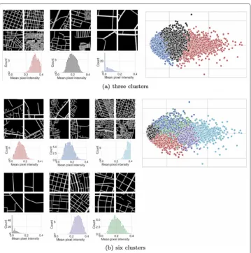
elbow method (Dangeti2017). As shown in Fig.6a, the obtained clusters seem to separate street networks based on their street density. We found further cluster characteristics by calculating their network metrics in Table1. The results in Table1show that the clusters can be clearly distinguished using network metrics such as node degree or average edge length. For example, the red cluster is composed of street networks with many short street segments, whereas the blue cluster contains street networks with much fewer but longer streets. The preliminary results suggest that theurban network vectorsused for clustering street images are capable of capturing key street network properties, hence they could be used to generate a diverse range of realistic urban forms.
When we increased the number of clusters toK =6 in Fig.6b, we could differentiate road networks based on more subtle network characteristics, such as disconnectedness of roads in the first cluster (top-left in Fig.6b) or large gaps in road provision in the sec-ond cluster (top-centre in Fig.6b). We visualised both cluster assignments in Fig.6(right) by projecting the thirty-two-dimensional urban network vectors to a two-dimensional grid using T-SNE algorithm (Maaten and Hinton 2008) for dimensionality reduction. The visualisations show that street networks cluster well into three groups that were detected by theK-means algorithm since the groups are well balanced in size and non-overlapping. The three clusters are further mapped to investigate spatial patterns in urban form variation (Fig.7).
Urban networks generation
Fig. 6aThree orbsix clusters of urban street forms obtained by applyingK-means algorithmto the condensed urban network vectors. Subfigures show example street networks in each cluster (top left), street network density in each cluster (bottom left) approximated using pixel intensity of street images, and a two-dimensional visualisation of all urban vectors with colour-coded cluster membership
encodehigh-dimensional observations as meaningful low-dimensional representations. The second strength pertains to the ability togeneraterealistic urban street forms that match the complexity of urban forms across the globe. The ability could potentially advance the current state-of-the-art in simulations of urban forms and socio-economic processes taking place on urban networks.
To generate a synthetic urban network, we firstly sample an embedding valuezfrom the prior distributionp(z)specified as a standard Gaussian (see “Variational autoencoder”
Table 1Average network metrics of urban street networks in the three clusters in Fig.6a
Network metric Cluster
Red Black Blue
Number of nodes 2488.5 1271.6 358.7
Number of edges 6671.1 3261.3 913.6
Average node degree 5.4 5.2 4.8
Total edge length 328975.6 207221.9 76841.7
Fig. 7Distribution of urban street forms across the globe. Each dot represents a city and is colour-coded according to cluster memberships in Figure6a. Despite limited data size, spatial trends start to emerge, such as the concentration of high-density urban networks in California, USA (red cluster) and low-density urban networks in south-eastern Asia (black cluster)
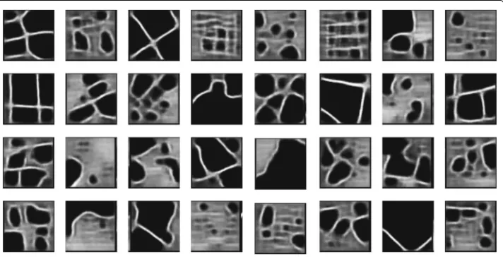
section) and then pass the value through the decoder network to obtain a correspond-ing image. Images correspondcorrespond-ing to several embeddcorrespond-ing samples are shown in Fig.8. As shown in the figure, the generated images lack the detail of real street images in Fig.3. Although the samples follow the general structure of road networks with major roads and areas of mixed-density minor roads, the decoder fails to reconstruct details of dense road segments and instead represents them blurred. The problem must be accredited to too few images used in the study. Although the proposed model is flexible enough to model urban street networks, which is confirmed by high-quality reconstructions of real images in Fig.4, it does not see enough images to learn to interpolate between them to sample new forms of street networks to sufficient detail.
Discussion and conclusions
This study is an early exploration of how modern generative machine learning mod-els such as variational autoencoders could augment our ability to model urban forms. With the ability to extract key urban features from high-dimensional urban imagery, vari-ational autoencoders open new avenues to integrating high-dimensional data streams in urban modelling. The study considered images of street networks, but the proposed methodology could be equally applied to other image data, such as urban satellite imagery. Variational autoencoders were selected among deep generative models (Moosavi2017; Albert et al. 2018) due to their two capabilities: firstly to condense images to low-dimensional representations, secondly to generate new previously unseen images that match the complexity of observed images. The first capability enabled us to extract key urban metrics from street network images, the second gave us the power to generate realistic images of previously unseen urban networks.
Our results, based on 12,479 city images across the globe, showed that VAEs suc-cessfully condensed urban images into low-dimensional urban network vectors. This enabled quantitative similarity analysis between urban forms, such as clustering. What is more, VAEs managed to generate new urban forms with complexity matching that of the observed data. Unfortunately, the resolution of the generated images was low which was accredited to the small size of the dataset. Future work will repeat model training on a much larger corpus of images to improve the generative quality. Moreover, further work will fine tune the generative quality by investigating the impact of the size of the latent space (currently fixed to 32 dimensions) and the training objective used (e.g. Wasserstein distance instead of KL divergence).
Despite the promising results, the study opens essential questions for future work. The first question pertains to the black-box nature of deep learning models that lack com-prehensive human interpretability. This limitation is already receiving much attention in the deep learning literature (Ribeiro et al. 2016; Shrikumar et al. 2017; Lundberg and Lee2017). In this study, the limitation manifests itself in our lack of understanding of how latent space representations of urban networks relate to established network met-rics (Newman2010). A related question refers to the ability to evaluate the quality of model outputs, i.e. latent representations and synthetic images. Again, quality assessment of deep generative models is a hot topic in the broader deep learning research commu-nity (see for example Wu et al. (2017)).Future work could address the problem from the perspective of urban network science. Finally, before this type of generative models could be part of any urban planning cycle, we need to reflect how we might develop these tools further through designing a structured set of experiments that include, for example, population densities or environmental features.
Acknowledgments
The authors would like to thank Szymon Zareba and Adam Gonczarek (Alphamoon Ltd) for advice on deep generative models during the course of the project.
Authors’ contributions
KK designed and implemented the methodology, executed the computer runs, and wrote the initial version of the article. RM prepared street network data and extensively revised the article. Both authors read and approved the final manuscript.
Authors’ information
RM is a senior research fellow at the Bartlett’s Centre for Advanced Spatial Analysis, University College London, UK. His academic interests include urban complex networks, information transfer in social systems, spatial interaction models and pedestrian flows. One of his main research topics is the application of multifractal measures to different urban aspects, such as street networks and social inequality.
Funding
There is no specific funding received for the study.
Availability of data and materials
All data and program source code described in this article is available to any interested parties. The source code and experiments are available at GitHub at the following URL:https://github.com/kirakowalska/vae-urban-network. The raw data and datasets generated during this study are available upon request.
Competing interests
The authors declare that they have no competing interests.
Received: 30 April 2019 Accepted: 13 November 2019
References
Albert A, Strano E, Kaur J, González M (2018) Modeling urbanization patterns with generative adversarial networks. In: IGARSS 2018-2018 IEEE International Geoscience and Remote Sensing Symposium. IEEE. pp 2095–2098
Arcaute E, Molinero C, Hatna E, Murcio R, Vargas-Ruiz C, Masucci AP, Batty M (2016) Cities and regions in britain through hierarchical percolation. R Soc Open Sci 3(4):150691.https://doi.org/10.1098/rsos.150691
Barthélemy M, Flammini A (2008) Modeling urban street patterns. Phys Rev Lett 100(13):138702
Boeing G (2018) A multi-scale analysis of 27,000 urban street networks: Every US city, town, urbanized area, and Zillow neighborhood. Environment and Planning B: Urban Analytics and City Science:2399808318784595
Buhl J, Gautrais J, Reeves N, Solé R, Valverde S, Kuntz P, Theraulaz G (2006) Topological patterns in street networks of self-organized urban settlements. Eur Phys J B-Condens Matter Complex Syst 49(4):513–522
Cardillo A, Scellato S, Latora V, Porta S (2006) Structural properties of planar graphs of urban street patterns. Phys Rev E 73(6):066107
Chu H, Li D, Acuna D, Kar A, Shugrina M, Wei X, Liu M-Y, Torralba A, Fidler S (2019) Neural turtle graphics for modeling city road layouts. In: Proceedings of the IEEE International Conference on Computer Vision. pp 4522–4530
Dangeti P (2017) Statistics for Machine Learning. Packt Publishing Ltd, Birmingham
Fukushima K (1980) Neocognitron: A self-organizing neural network model for a mechanism of pattern recognition unaffected by shift in position. Biol Cybern 36(4):193–202
Haklay M, Weber P (2008) Openstreetmap: User-generated street maps. IEEE Pervasive Comput 7(4):12–18 Kingma DP, Welling M (2014) Auto-encoding variational bayes
Krizhevsky A, Sutskever I, Hinton GE (2014) Imagenet classification with deep convolutional neural networks. In: Neural Information Processing Systems. pp 1097–1105
LeCun Y, Bengio Y, et al. (1995) Convolutional networks for images, speech, and time series. Handb Brain Theory Neural Netw 3361(10):1995
LeCun Y, Boser BE, Denker JS, Henderson D, Howard RE, Hubbard WE, Jackel LD (1990) Handwritten digit recognition with a back-propagation network. In: Adv Neural Inf Process Syst. NIPS. pp 396–404
Levinson D (2012) Network structure and city size. PloS ONE 7(1):29721
Li Z, Wegner JD, Lucchi A (2018) Polymapper: Extracting city maps using polygons. arXiv preprint arXiv:1812.01497 Lundberg SM, Lee S-I (2017) A unified approach to interpreting model predictions. In: Advances in Neural Information
Processing Systems, NIPS. pp 4765–4774
Maaten Lvd, Hinton G (2008) Visualizing data using t-sne. J Mach Learn Res 9(Nov):2579–2605
Masucci AP, Smith D, Crooks A, Batty M (2009) Random planar graphs and the london street network. Eur Phys J B 71(2):259–271
Máttyus G, Luo W, Urtasun R (2017) Deeproadmapper: Extracting road topology from aerial images. In: Proceedings of the IEEE International Conference on Computer Vision. IEEE. pp 3438–3446
Moosavi V (2017) Urban morphology meets deep learning: Exploring urban forms in one million cities, town and villages across the planet. arXiv preprint arXiv:1709.02939
Murcio R, Massuci AP, Arcaute E, Batty M (2015) Multifractal to monofractal evolution of the london street network. Phys Rev E 92(6):2130.https://doi.org/10.1103/PhysRevE.92.062130
Newman M (2010) Networks: an Introduction. Oxford university press, Oxford
Peponis J, Allen D, French S, Scoppa M, Brown J (2007) Street connectivity and urban density. In: 6th International Space Syntax Symposium. Citeseer, Istanbul. pp 1–12
Ribeiro MT, Singh S, Guestrin C (2016) “Why should I trust you?”: Explaining the predictions of any classifier. In: Proceedings of the 22nd ACM SIGKDD International Conference on Knowledge Discovery and Data Mining, San Francisco, CA, USA, August 13-17, 2016
Shrikumar A, Greenside P, Kundaje A (2017) Learning important features through propagating activation differences. In: Proceedings of the 34th International Conference on Machine Learning
Strano E, Viana M, da Fontoura Costa L, Cardillo A, Porta S, Latora V (2013) Urban street networks, a comparative analysis of ten european cities. Environ Plan B Plan Des 40(6):1071–1086
Witten IH, Frank E, Hall MA, Pal CJ (2016) Data Mining: Practical Machine Learning Tools and Techniques. Morgan Kaufmann, Burlington
Zhao F, Sun H, Wu J, Gao Z, Liu R (2016) Analysis of road network pattern considering population distribution and central business district. PloS ONE 11(3):0151676
Publisher’s Note