Reactive Power Optimization Based on Parallel Immune Particle Swarm Optimization

Reactive Power Optimization Based on Parallel

Immune Particle Swarm Optimization

Guili Yuan

School of Control and Computer Engineering North China Electric Power University, Beijing, China

Email:[email protected]

Lei Zhu and Tong Yu

School of Control and Computer Engineering North China Electric Power University, Beijing, China Email: {[email protected], [email protected]}

Abstract—Reactive power optimization is important to ensure power quality, improve system security, and reduce active power loss. So, this paper proposed parallel immune particle swarm optimization (PIPSO) algorithm. This algorithm makes basic particle swarm optimization (BPSO) and discrete particle swarm optimization (DPSO) to optimize in parallel, and improves the convergence capability of particle swarm optimization with convergence ability. It is effective to overcome the problem of local convergence by immune operator, at the same time, it is more reasonable to solve the complex coding problem which discrete variables and continuous variables mixed by parallel optimization. Finally, the simulation results of IEEE-14, IEEE-30, IEEE-118 nodes system show that compared to the genetic algorithm and basic particle swarm optimization, the parallel immune particle swarm optimization can achieve the convergence effect faster and more stable, and better to solve the large-scale power system reactive power optimization.

Index Terms—reactive power optimization, particle swarm optimization, immune algorithm, discrete algorithm, parallel optimization

I. INTRODUCTION

Reactive power optimization of power system is a real integer mixed nonlinear programming problems with multi-objective, multi-variable, multi-constraint. Its optimization variables consists of both continuous variables such as the node voltage of generator and discrete variables such as transformers regulator stalls and the number of reactive power compensation device, which makes the whole process very complicated especially dealing with the discrete variables . Reasonableness of the reactive power flow distribution not only connects to the quality of the power provided, but also directly affects the safety of operation of the power grid itself and the economy. Therefore, reactive power optimization has always been a hot topic of research. For years scholars have proposed a series of solutions, such as linear programming, nonlinear

programming, interior point method, and the intelligent optimization methods widely studied in recent years. These traditional methods have stable data and reliable convergence; but difficult to deal with discrete variables, easy to fall into local optimum and cause errors [1]. With the development of computer and optimization technology, a variety of intelligent optimization algorithms have been applied to reactive power optimization problems, such as Simulated Annealing algorithm [2], Taboo search algorithm [3] ,Genetic Algorithm [4], Immune Algorithm [5,6],Particle Swarm Optimization[7,8].These intelligent algorithms have good convergence with lower request of the objective function, which makes up some flaws of the traditional reactive power optimization algorithm to some extent. But with increase of the scale and complexity of the reactive power optimization problem, these intelligent algorithms still have the disadvantages of computing for a long time and easy to fall into local optimum [9] .Single algorithm has gradually unable to meet the requirements for solving problems. So many scholars applied hybrid intelligent optimization algorithm to reactive power optimization problem [10, 11].

II.MATHEMATICAL MODEL OF REACTIVE POWER

OPTIMIZATION

The purpose of reactive power optimization is to reduce active power consumption, while ensuring the node voltage and generator output at the best level on condition that power flow has been scheduled with generator terminal voltage amplitude, reactive power compensation capacity of reactive power compensation device and load tap transformer ratio as a control variable, reactive power of generators and the voltages of load nodes as state variables.

A. Objective Function

The objectives function of reactive power optimization such as formula (1) [14].

lim lim

, ,

2 2

1 ,max ,min 1 , ,max , ,min

min V( ) G( )

N N

G i G i i i

L u Q

i i i i G i G i

Q Q

V V F P

V V Q Q

λ λ = = − − = + + − −

∑

∑

,max ,max

lim

,min ,min

, ,max , , ,max

lim ,

, ,min , ,min

i i i

i

i i i

G i G i G i

G i

G i G i Gi

V V V

V

V V V

Q Q Q

Q

Q Q Q

⎧ _⎧⎪ ≥ = ⎪ ⎨ ≤ ⎪ ⎪ ⎩ ⎨ ≥ ⎧ ⎪ ⎪ =⎨ ⎪ _≤ ⎪⎩ ⎩ ， ， ， ，

WhereP_L is the active power loss andV_i,V_i,max, V_i,min are voltage of the nodes and theirs upper and lower limits.

,

G i

Q ,QG i, ,max,QG i, ,minare reactive power injected by the

gene- rator nodes and theirs upper and lower limits. NVis the total number of nodes. N_G is the total number of generators.

The Item 2 and 3 in the formula (1) are the out-of-limit penalty functions of node voltages and generator reactive power to ensure the best level of node voltages and the generator output. The penalty coefficients_λu, _λQ take the principle of dynamic values of the exponentially[15].

max max max , , Iter α λ λ λ λ λ λ ⎧ _< ⎪ =⎨ ≥

⎪⎩ (2) Where α is the base, Iter is the evolutionary algebra and

max

λ is the upper limit ofλ . In this way, λ values smaller in the early evolution of population and P_L can occupy larger proportion in the objective function, which can accelerate the convergence speed. In the latter part of the algorithm, as λ increases, the objective function value of violating the restrictions will deteriorate which not only satisfies the requirements of the penalty function, but also gets the minimum solutions.

B. Constraint Conditions Power flow constraint formula

1

1

( cos sin )

( sin cos )

i i

i i

n

G D i j ij ij ij ij

j n

G D i j ij ij ij ij

j

P P V V G B

Q Q V V G B

θ θ θ θ = = ⎧ = + + ⎪ ⎪ ⎨ ⎪ _{= + −} ⎪ ⎩

∑

∑

WhereP_Gi, Q_Gi are the active and reactive power outputs of generator nodes. P_Di , Q_Di are active and reactive load

power of load nodes. nis the total number of nodes. V_i, j

V are the voltage amplitude of nodes i, j.Gij, Bijare the conductance and susceptance between node i and node j.

ij

θ is the voltage phase angle between node i and node j. Variable constraints

Inequality constraints of the control variables and inequality constraints of the state variables are included as followed.

min max

min max

min max

b b b

r r r

g g g

T T T

C C C

V V V

⎧ _{< <} ⎪

< < ⎨

⎪ _{< <} ⎩

(4)

min max

, ,min , , ,max

i i i

G j G j G j

V V V

Q Q Q

< < ⎧⎪

⎨ _{< <}

⎪⎩ (5) Where Tb is the transformer ratio and Tb,max , Tb,min are the upper and lower limits. Cr is compensation capacitor capacity; and Cr,max, Cr,min is the upper and lower limits. Vg is generator terminal voltage and Vg,max, Vg,minis the upper and lower limits.Vi is node voltage of system and Vi,max, Vi,min is the upper and lower limits . QG,j is generator reactive power output and QG,j,max, QG,j,min is the upper and lower limits. b,

r , g are the number of transformers, reactive compensation nodes and generators.

III. FLOW OPTIMIZATION OF POWER SYSTEM INCLUDING

WIND FARM

At present, China’s wind turbine mainly is fixed pitch, asynchronous set. In theory, the wind turbine node is neither the PV node nor the PQ node. The relationship of wind turbine output power and wind speed [16] such as formula (6): 3 3 3 3 0, , , , cin cout cin

r cin r

r cin

r r cout

v v v v

v v

P P v v v

v v

P v v v

< >

⎧ ⎪

− ⎪

=⎨ ≤ <

− ⎪

⎪ _{≤ ≤}

⎩

(6)

Wherevis wind speed at the wind turbine hub, P is the active power output of wind turbine; v_cin, v_r,

cout

v , are cut-in speed, rated wind speed, cut- out wind speed and rated power of wind turbine; It can be drawn the output of each wind turbine in different wind speeds, the slip ratio of induction motor can be calculated by the power P and the wind turbine machine terminal voltage U .

2 4 2 2 2 2

2

4 2

U R U R P x R

s

Px

σ σ

− −

= (7)

Similarly, the induction generator output reactive power can be expressed as:

2 2

[ ( m ) ]

m

R x x x s P

Q

sRx

σ σ

+ +

= (8)

which the wind turbines need to absorb. In the load flow calculation, according to the formula (8), modify the traditional power flow correction formula. Reference [16] has given the corresponding expression.

IV. PARTICLE SWARM OPTIMIZATION

Particle Swarm Optimization is an evolutionary computing technology based on swarm intelligence proposed by Kennedy and Eberhan in 1995 [17] .They observed the behaviors of birds in the process of searching food and simplified model of this community. Particle Swarm Optimization applied swarm intelligence produced by cooperation and competition between particles to guide the search of optimization, finally, the optimal solution of the problem is found.

A. Standard Particle Swarm Optimization

In the Standard Particle Swarm Optimization, flock of birds was abstracted as particles without mass and volume, as feasible solutions of the optimization problem. Each particle has a fitness value determined by the objective function; there also is a speed to determine their fly direction and distance. Particles update themselves to approximate the optimal value by tracking two "extreme values" during the flight. One is the best position found by themselves, called individual extreme. the other is found by the whole group, called global extreme. This process is mathematically described as: assuming an n-dimensional space, population consist of m particles, X={x1, … , xi,…,xm}. The position of i-th particle is xi=(xi1,xi2, …,xin), and the corresponding speed is vi=(vi1,vi2, …,vin). According to the principle of particle flight, particles will update position and rate by equation (9).

1 1 1 2 2

1 1

( ) ( )

k k k k k k

k k k

v v c r pbest x c r gbest x

x x v

ω + + + = + − + − ⎧ ⎨ = + ⎩ (9)

Where ωis inertia factor, c1, c2 are learning factors and r1,r2 are random numbers between [0, 1]. Inertia weight ω

decides the previous speed affecting the current speed and can balance the global search and local search of the algorithm. To improve the optimization performance of the algorithm, we use exponentially decreasing weights.

2 ( ) max min ( ) Iter a MaxIter Iter e

ω = ω −ω × − • (10) Where _ωmax is the maximum weight factor and _ωmin is the minimum weight factor. a is descending coefficient, generally takes [25,50]. Iter is the current iteration and MaxIter is the total algebra.

The PSO take a great advantage of the optimization process on continuous variables; but reactive power optimization problem is a mixed problem of continuous and discrete variables. In order to solve the discrete problem, this paper introduces a discrete particle swarm optimization algorithm.

B. Discrete Particle Swarm Optimization

Clerc proposed the DPSO based on the exchange in 2002[18] .This algorithm uses finite elements in discrete variables set to be exchanged. In DPSO, a position represents a discrete-element vector; a velocity represents the exchange of elements. Because the transform form of the speed is changed, the formulas of PSO need to be changed, too.

(1) Positions subtraction (Θ): Two positions subtract get a new speed.

1, 2, 2, 1, 2, 0 , i i

i i i

i

x x

v x x

x other = ⎧⎪ = Θ =⎨ ⎪⎩ ， (11)

(2) Coefficient and speed multiply (:): Coefficient and speed multiply only change the size of the speed. Assume a learning factor is c and make c’ as a random number between (0, 1).

1, 2, 1,i , ' v 0, i i

v c c

v c other < ⎧ = =⎨ ⎩

: (12)

(3) Speed addition (⊕): Two speeds adding together still get speed. 1, 2, 1, 1, 2, 1, 2, 2,

0 & 0 ,

0 & 0 & 0.5 ,

i i

i

i i

i i i

i

v v

v

v v rand

v v v

v other

⎧ ⎧⎪ ≠ =

⎪ ⎨ _{≠ ≠ <}

= ⊕ =⎨ ⎪⎩

⎪ ⎩

）

(13)

(4) Position and speed addition (¤): Position and speed adding together get a new position.

, 0

¤

, 0

i i

i i i

i i

v v

x x v

x v

≠ ⎧

= =⎨

=

⎩ (14) After redefine all kinds of operations, the updating formulas of PSO turn into these new formulas.

1 1 2

1 1

( ) ( )

¤

k k k k k k

k k k

v v c pbest x c gbest x

x x v

ω + + + = ⊕ Θ ⊕ Θ ⎧ ⎨ ₌ ⎩ : : : (15)

V. PARALLEL IMMUNE PARTICLE SWARM OPTIMIZATION The control variables of reactive power optimization consist of continuous variables and discrete variables. Since the dimension of the control variables is large, if adopt the conventional binary encoding, the particle’s code length is large. This makes the search space expanded dramatically and results in "curse of dimensionality". Meanwhile, it will produce large errors in the process of continuous variables and discrete variables in mutual transformation and affects the accuracy.

optimization for dealing with discrete variables can solved effectively and the searching efficiency and solution accuracy are improved.

A. The diversity of Particle Swarm

To increase the diversity of the population, new particles are generated by the following two aspects in each generation of the evolutionary process.

(1) New particles are generated by the PSO updating formula (9) and formula (15).

(2) New particles are generated randomly in the search space.

In order to ensure the diversity of particles, we adopt the concentration promote inhibition mechanism based on vector distance [19], so that in the new populations, the each fitness level of particles to maintain a certain concentration. This selection probability based on the concentration and fitness is called viability. The viability of the i-th particle is given by equation formula (16).

1

1

1 1

( ) ( ) (1 )

( )

( ) ( ) (1 )

( ) ( ) i

s i f N

i i

N

i j

j

f N N

i j

i j

x

P x P

x

f x f x P

f x f x ρ

α α

ρ

α α

=

=

= =

= − × + ×

−

= − × + ×

−

∑

∑

∑∑

(16)

Where f x ( )_i is the fitness of the i-th particle and Pf is the individual selection probability based on fitness.α is the concentration attenuation coefficient, 0<α<1. N is the population size. This approach makes particles with low-fitness get the opportunity to evolve and improves the diversity of population.

B. Vaccines Operator

Vaccines operator can guide the search process, improve optimal performance and suppress the degradation through the extract vaccine and vaccination. (1) Vaccines Operator

After a certain generation optimized, the individual gene fragments of the optimal solution in population will appear in some antibodies, these fragments can be used as a vaccine extracted and inoculated to the other antibodies. Assume that there are s fragments k1,k2,…,ks can be chosen in each gene of each antibody, the probability of the fragment is kj on the i allele in the population such as the formula:

,

1

1

1, ( ) 0,

N

i j j

j

j j

p a

N g i k a

other = ⎧

= ⎪ ⎪ ⎨

= ⎧⎪ ⎪ ₌

⎨ ⎪ _⎪⎩ ⎩

∑

(17)

Where ( )g i is the symbol on the i allele, N is the population size. The kj is a fragment on the allele that maximum probability greater than a set threshold Tb. To improve the extraction efficiency of vaccine, the

threshold value Tb increased linearly with the generation The final extracted vaccine is as the following formula:

1 2

,

( , , ) , max( ) 0,

n

j i j b

j

B b b b

k p T

b

other =

⎧ ⎪

≥ ⎧

⎨ ⎪ =⎨ ⎪

⎪⎩ ⎩

"

(18)

(2) Vaccination

According to the vaccination probability Pc, the individuals from parent groups to be vaccinated are selected. Then we access the vaccine gene fragments into the chosen particles in turn, and eventually form a new population. Probability of vaccination is expressed as follows.

, 1

( )

1, 1 best

avg

best avg

c

f f

u f

f uf

P u

f u

− ⎧

≤

⎪ ₋

=⎨ =

⎪ _> ⎩

(19)

Where f_bestis the best fitness and f_avgis the average fitness.

C. The Reactive Power Optimization Step based on PIPSO

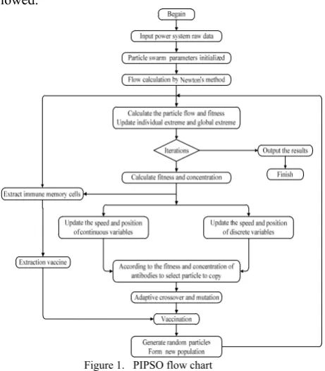
The flow chart and specific steps are shown as followed.

Figure 1. PIPSO flow chart (1) Input power system raw data.

(2) Initialize the population parameters and form the initial population and initial extremes.

(3) Calculate the power flow of the particles in the initial population.

(4) According to the results of flow calculation, calculate the fitness and viability of population, then update the extreme.

(6) According to formula (9) and (15) to update the speed and position of the particle. (7) Select and copy the particles according to the viability.

(8) Self-adaptive crossover and mutation operations on the population after the copy, then vaccination.

(9) Randomly generated part of particles and formed a new population with the particles in the population after vaccination and memory cells

(10) Calculate the flow of new population.

(11) If it fails to reach convergence conditions, return to step (5); otherwise terminate the computation.

VI.SIMULATION

The parallel immune particle swarm algorithm is applied to the reactive power optimizations of standard

IEEE-14 bus system, IEEE-30 bus system and standard IEEE-118 bus system. The results are compared with that optimized by standard particle swarm optimization and genetic algorithm. Set population size as 30. Crossover probability of GA is 0.9 and mutation probability decreases linearly in [0.1, 0.01]. Standard particle swarm optimization and parallel immune particle swarm

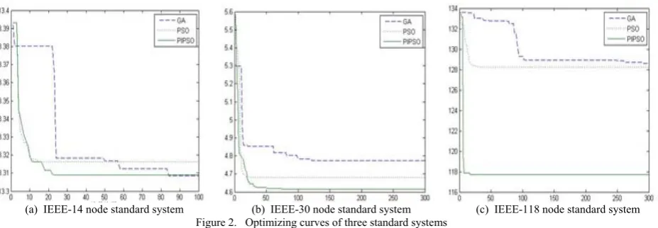
The results of the three different optimization algorithms corresponding to the three systems are shown in Table 2. Net loss optimized and computing time are the average obtained by several calculating. Optimizing curves of different methods are shown in Fig. 2.

TABLE 1.

PARAMETER VALUES OF TEST SYSTEMS

Test system System load Generator terminal voltage /V Transformer ratio Step Shunt capacitance Step

P/MW Q/MVar Vmax Vmin Tmax Tmin a Dmax Dmin b

IEEE-14 259.00 73.50 1.06 0.94 1.10 0.95 0.015 50 0 10

IEEE-30 299.40 127.03 1.1 0.95 1.10 0.95 0.015 50 10 0 10 2

IEEE-118 4242.0 1438.0 1.06 0.94 1.01 0.91 0.025 30 20 0 0 0 -50 10 2 -5

TABLE 2

.REACTIVE POWER OPTIMIZATION RESULTS OF THE THREE SYSTEMS.

System IEEE-14 IEEE-30 IEEE-118

Algotithm Net loss (MW)

Convergence algebra

Loss reduced 104_yuan/year

Net loss (MW)

Convergence algebra

Loss reduced 104_yuan/year

Net loss (MW)

Convergence algebra

Loss reduced 104_yuan/year

GA 13.335 53.3 16.7543 5.004 172.4 166.7383 129.14 179.9 1069.775

BPSO 13.332 21.9 17.4153 4.823 70 218.6968 129.35 50.4 1009.655

PIPSO 13.311 25 23.5078 4.628 87.8 274.8510 117.83 20.7 4319.132

Set the average price of system is 571.22 Yuan / MWh and annual average utilization hour is 5,031 hours. Loss reduced = Net loss before optimized * price * time - Net loss optimized * price * time

(a) IEEE-14 node standard system (b) IEEE-30 node standard system (c) IEEE-118 node standard system Figure 2. Optimizing curves of three standard systems

From Table 2, parallel immune particle swarm optimization proposed in this paper has advantages on the effect and speed, and with the scale and complexity of the system increasing, the advantages are more obvious. It can be seen from Fig. 2 (a) that PIPSO improves the diversity of the population by taking advantage of

to effectively obtain the optimal solution, while PIPSO shows stable and efficient convergence. Therefore PIPSO can be applied to solve large-scale system reactive power optimization problem.

PIPSO is applied to a regional power system reactive power optimization. the system size is 2,383 nodes, 2,896 branches, 327 generators nodes, terminal voltage can be adjusted, 170 sets of variable transformer. Upper and lower load node voltage per unit of 1.10 and 0.94, with a total load of P = 24558.38 MW, Q = 8143.92 MVar. Optimizing curve is shown in Fig. 3.

Figure 3. Optimizing curve of a practical system

Before optimization, the active power loss of actual system is 722.5870MW. While active power loss optimized by PIPSO reduced to 689.8696MW.The annual economic loss after optimization can reduce 94,023,520 Yuan. It can be seen that desired results can be achieved fast and stalely with PIPSO dealing with large network.

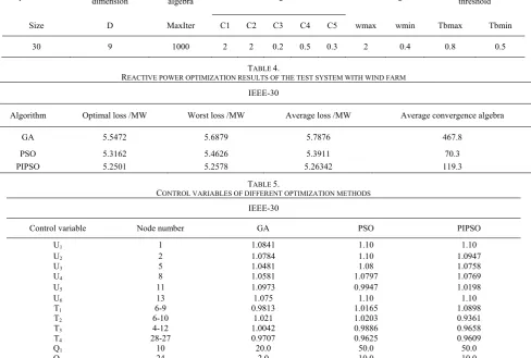
The wind farm of this paper is as follows: Assume that the wind farm respectively accesses to the No. 3 of IEEE-30 system through the 110kV line. The wind farm transmission impedance is 3.14963 + j6.23997Ω; the wind farm capacity is 20 × 800KW; the stator leakage reactance is 0.07620Ω and the rotor impedance is 0.00759 + j0.18289Ω; the excitation reactance is 3.44979Ω. Assume that the wind farm wind speed is the rated wind speed. The parameters of algorithm are shown in Table 3. GA, PSO and PIPSO are applied to calculate the reactive power optimization respectively. The results are shown in Table 4 and Table 5.

TABLE 3. PIPSO PARAMETERS

Population size Population _dimension Iterative _algebra Learning factor Inertia weight Vaccine extract _threshold

Size D MaxIter C1 C2 C3 C4 C5 wmax wmin Tbmax Tbmin

30 9 1000 2 2 0.2 0.5 0.3 2 0.4 0.8 0.5

TABLE 4.

REACTIVE POWER OPTIMIZATION RESULTS OF THE TEST SYSTEM WITH WIND FARM

IEEE-30

Algorithm Optimal loss /MW Worst loss /MW Average loss /MW Average convergence algebra

GA 5.5472 5.6879 5.7876 467.8

PSO 5.3162 5.4626 5.3911 70.3

PIPSO 5.2501 5.2578 5.26342 119.3

TABLE 5.

CONTROL VARIABLES OF DIFFERENT OPTIMIZATION METHODS

IEEE-30

Control variable Node number GA PSO PIPSO

U1 1 1.0841 1.10 1.10

U2 2 1.0784 1.10 1.0947

U3 5 1.0481 1.08 1.0758

U4 8 1.0581 1.0797 1.0769

U5 11 1.0973 0.9947 1.0198

U6 13 1.075 1.10 1.10

T1 6-9 0.9813 1.0165 1.0898

T2 6-10 1.021 1.0203 0.9361

T3 4-12 1.0042 0.9886 0.9658

T4 28-27 0.9707 0.9625 0.9609

Q1 10 20.0 50.0 50.0

Figure. 4 The optimizing curves of GA, PSO, PIPSO

The convergence curves of the objective functions of the three algorithms are shown in Figure 4. It can be seen from Figure 4, PIPSO can converge to a better solution. At the same time, the decline rate in the beginning of PIPSO is very quick. It is because the vaccines operator will extract the good genes from memory cells which improve particles. Later in the algorithm, the vaccines have been close to the optimal solution, and the immunization effect will become more apparent, so improve the convergence accuracy and the optimization ability in the later stage of evolution. These comparison shows that PIPSO had better global convergence ability, and solved the encoding problem of the discrete variables. It is a feasible algorithm for large and complex reactive power optimization problem.

VII.CONCLUSION

In this paper, parallel immune particle swarm algorithm is designed for reactive power optimization. The problem easy to fall into local optimum of particle swarm algorithm can be improved by parallel optimization of standard particle swarm optimization and discrete particle swarm optimization with using immune operator to improve the diversity of the algorithm. The simulation shows the parallel immune particle swarm algorithm can find the global optimal solution fast with more accurate convergence. The performance of solving large-scale power system reactive power optimization problem is particularly prominent. It has theoretical and practical significance.

ACKNOWLEDGMENT

In this paper, the research was sponsored by National Natural Science Foundation (NNSF) of China (61240037) and the Central Universities Youth Fund (11QG11).

REFERENCES

[1] Xu Wenchao, Guo Wei. Summarize of Reactive Power Optimization Model and Algorithm in Electric Power System [J].Proceedings of the Chinese Society of Universities for Electric Power System and Automation, 2003, 1(15):100-104.

[2] Liang R H, Wang Y S. Main transformer ULTC and capacitors scheduling by simulated annealing approach [J]. Electrical Power and Energy Systems, 2001, 23(7):531-538. [3] Wen E S, Chang C S. Tabu search approach to alarm processing in power systems [J].IEE Proceedings-Generation, Transmission and Distribution, 1997, 144(1):31-38.

[4] Zeng X, Tao J, Zhang P, et al. Reactive Power Optimization of Wind Farm based on Improved Genetic Algorithm [J]. Energy Procedia, 2012, 14: 1362-1367. [5] Lin J, Wang X. Reactive power optimization based on

adaptive immune algorithm [J].International Journal of Emerging Electric Power Systems, 2009, 10(4).

[6] Xiong Hugang, Cheng Haozhong, Li Hongzhong. Multi-objective reactive power optimization based on immune algorithm [J].Proceedings of the CSEE, 2006, 26(11):104-108(in Chinese).

[7] xiao-hua W, yong-mei Z. Multi-Objective Reactive Power Optimization Based On The Fuzzy Adaptive Particle Swarm Algorithm[J]. Procedia Engineering, 2011, 16: 230-238.

[8] Mahadevan K, Kannan P S. Comprehensive learning particle swarm optimization for reactive power dispatch [J]. Applied soft computing, 2010, 10(2): 641-652.

[9] Hao Xiaohong, Zhang Yang. Summarize of Intelligent Optimization Algorithms in Reactive power optimization [J].Industrial Instrumentation & Automation, 2010, 2:12-15.

[10] Subbaraj P, Rajnarayanan P N. Hybrid particle swarm optimization based optimal reactive power dispatch [J]. International Journal of Computer Applications, 2010, 1(5): 65-70.

[11] Zhaoyu P, Shengzhu L, Nan Z. The Application of Adaptive PSO in Power Reactive Optimization [J]. Procedia Engineering, 2011, 23: 747-753.

[12] Shao B, Liu J, Huang Z, et al. A Parallel Particle Swarm Optimization Algorithm for Reference Stations Distribution [J]. Journal of Software (1796217X), 2011, 6(7).

[13] Xu H, Yang Y, Mao L. Study and Improvement on Particle Swarm Algorithm [J]. Journal of Computers, 2013, 8(4). [14] Lin Ji-keng, Li Hong-lu, Luo Shan-shan, Zheng Wei-hong.

Reactive Power Optimization of Power System Based on Adaptive Immune Algorithm [J].Journal of Tianjin University.2007,1(40): 110-115

[15] Zhang Wujun, Ye Jiangfeng, Liang Weijie, Fang Gefei. Multiple- Objective Reactive Power Optimization Based on Improved Genetic Algorithm [J].Power System Technology.2004, 11(28):67-71.

[16] Liu Yang, Li Zhi, Zhang Bo, Han Xueshan. ‘Power Flow Study of Wind Power Accessing into Grid’. New Energy Power Generation. pp.2679-2682

[17] Kennedy J, Eberhart R. Particle swarm optimization [C]. Pro IEEE Int. Conf on Neural Networks. Perth, 1995, 1942-1948.

[18] Clerc M, Kennedy J. The particle swarm-explosion, stability, and convergence in a multidimensional complex space [J]. Evolutionary Computation, IEEE Transactions on, 2002, 6(1): 58-73.

Guili Yuan received the MS degree in

automation from North China Electric Power University in 2001, and the PHD degree in Thermal Engineering from the department of Thermal Engineering, North China Electric Power University in 2010. She is an associate professor in North China Electric Power University. Her research interests are in the areas of information control, advanced control strategies and their application in industrial processes.

Lei Zhu received master degree in automation from North

China Electric Power University in 2012 and her research is reactive power optimization.

Tong Yu is a master from North China Electric Power